2.1. Analytical and approximate equations for the mean wall-normal velocity

The mean wall-normal velocity plays a significant role in TBLs, as it characterizes the rate at which fluid is transported perpendicular to the wall. In this study, we derive an analytical equation for the mean wall-normal velocity from the integration of the dimensionless mean continuity equation. Previous research by Wei & Klewicki (Reference Wei and Klewicki2016) has identified the proper length and velocity scales for the mean wall-normal velocity in a ZPG TBL as $\delta _e$ and $V_e$, respectively. The variables in the mean continuity equation are normalized as

(2.2a–d)\begin{equation} x^* \mathop{=}\limits^{\rm def} \frac{x}{L}, \quad y^- \mathop{=}\limits^{\rm def} \frac{y}{\delta_e(x)}, \quad U^- \mathop{=}\limits^{\rm def} \frac{U_e - U(x,y)}{U_e}, \quad V^- \mathop{=}\limits^{\rm def} \frac{V(x,y)}{V_e(x)}, \end{equation}

where $L$ is a length scale in the $x$-direction, e.g. the computational domain size in the $x$-direction or the length of test section in a wind tunnel. Note that in a ZPG TBL, ${\rm d}U_e/{{\rm d}\kern 0.06em x}=0$ because $U_e$ is a constant, but $\delta _e$ and $V_e$ vary in the $x$-direction. It is worth highlighting that the dimensional velocity components $U$ and $V$ are functions of $x$ and $y$. In contrast, the normalized velocity components $U^-$ and $V^-$ are dependent on the normalized spatial variables $x^*$ and $y^-$.

Using the normalized variables $x^*$, $y^-$ and $U^-$, the $\partial U/\partial x$ term in the mean continuity equation can be written as

(2.3)\begin{equation} \frac{\partial U}{\partial x} = \frac{\partial (U_e - U_e U^-)}{\partial x} ={-}\frac{U_e}{L}\, \frac{\partial U^-}{\partial x^*} + \frac{U_e}{\delta_e}\,\frac{{\rm d}\delta_e}{{\rm d}\kern 0.06em x}\, y^-\,\frac{\partial U^-}{\partial y^-}. \end{equation}

Note that in the derivation of Wei & Klewicki (Reference Wei and Klewicki2016), an implicit self-similarity assumption is made that omits the $\partial U^-/\partial x^*$ term in (2.3). The importance of the streamwise derivative term has been recognized by Perry, Marusic & Jones (Reference Perry, Marusic and Jones2002), who incorporated it into the second term in their (2.9) (with $\zeta$). Disregarding this term is similar to assuming a constant Coles wake factor ($\varPi$, as defined by Coles Reference Coles1956) for ZPG TBLs. Although this assumption is a reasonable approximation, it is not strictly valid at finite Reynolds numbers.

By substituting the normalized variables in (2.2a–d) and (2.3) into (2.1a), the mean continuity equation becomes

(2.4)\begin{equation} 0 ={-}\frac{U_e}{L}\,\frac{\partial U^-}{\partial x^*} + \frac{U_e}{\delta_e}\, \frac{{\rm d}\delta_e}{{\rm d}\kern 0.06em x}\,y^-\,\frac{\partial U^-}{\partial y^-} + \frac{V_e}{\delta_e}\, \frac{\partial V^-}{\partial y^-}. \end{equation}

To obtain a dimensionless continuity equation, we multiply both sides of (2.4) by $\delta _e/V_e$:

(2.5)\begin{equation} 0 ={-}\frac{U_e}{V_e}\,\frac{\delta_e}{L}\, \frac{\partial U^-}{\partial x^*} + \frac{U_e}{V_e}\,\frac{{\rm d}\delta_e}{{\rm d}\kern 0.06em x} \left( \frac{\partial (y^- U^-)}{\partial y^-} - U^- \right) + \frac{\partial V^-}{\partial y^-}. \end{equation}

An analytical equation for the mean wall-normal velocity in a ZPG TBL can be obtained by integrating (2.5) with respect to $y^-$, starting from the wall:

(2.6)\begin{equation} V^- = \frac{U_e}{V_e}\,\frac{{\rm d}\delta_e}{{\rm d}\kern 0.06em x} \left( \int_0^{y^-} U^- {{\rm d} y}^- - y^-U^- \right) + \int_0^{y^-} \frac{U_e}{V_e}\,\frac{\delta_e}{L}\,\frac{\partial U^-}{\partial x^*}\,{{\rm d} y}^-. \end{equation}

The global integral of the mean continuity equation can be obtained by evaluating (2.6) at the boundary layer edge:

(2.7)\begin{equation} 1 = \frac{U_e}{V_e}\,\frac{{\rm d}\delta_e}{{\rm d}\kern 0.06em x} \int_0^{1} U^- {{\rm d} y}^- + \frac{U_e}{V_e}\,\frac{\delta_e}{L} \int_0^{1} \frac{\partial U^-}{\partial x^*}\,{{\rm d} y}^-. \end{equation}

Note that by definition, $\int _0^{1} U^-\,{{\rm d} y}^- =\delta _1/\delta _e$, where $\delta _1$ is the mass displacement thickness (see Schlichting Reference Schlichting1979). Therefore, the global integral equation (2.7) can be rewritten as

(2.8)\begin{equation} 1 = \frac{U_e}{V_e} \left( \frac{{\rm d}\delta_e}{{\rm d}\kern 0.06em x}\,\frac{\delta_1}{\delta_e} + \frac{\delta_e}{L} \int_0^{1} \frac{\partial U^-}{\partial x^*}\,{{\rm d} y}^- \right). \end{equation}

By applying the Leibniz integral rule to $\int _0^1 ({\partial U^-}/{\partial x^*})\,{{\rm d} y}^-$, an exact equation for $V_e$ is obtained from (2.8) as follows:

(2.9)\begin{equation} V_e = U_e\,\frac{\mathrm{d} \delta_1}{\mathrm{d}\kern 0.06em x}. \end{equation}

In many experimental studies, determining accurately $\mathrm {d} \delta _e/\mathrm{d}\kern 0.06em x$ or $\partial U^-/\partial x^*$ is often challenging due to the limited resolution in the streamwise direction. However, reliable and accurate determination of $\delta _e$, especially $\delta _1$, can be obtained. In the case of numerical simulation, two-dimensional mean field data must be available in order to calculate $\mathrm {d} \delta _e/\mathrm{d}\kern 0.06em x$ or $\partial U^-/\partial x^*$. Certain archived direct numerical simulation data include only mean profiles at discrete Reynolds numbers, which do not provide the necessary information to calculate $x$-derivatives. To obtain an approximate equation that can be determined more easily, the exact (2.6) is rearranged as

(2.10)\begin{align} V^- & = \frac{\delta_e}{\delta_1} \int_0^{y^-} U^-\,{{\rm d} y}^-- \frac{\delta_e}{\delta_1}\,y^-U^- \nonumber\\ &\quad + \left\{ \left( \frac{\mathrm{d}\delta_e/\mathrm{d}\kern 0.06em x}{\mathrm{d} \delta_1/\mathrm{d}\kern 0.06em x} - \frac{\delta_e}{\delta_1} \right) \left(\int_0^{y^-} U^-\,{{\rm d} y}^-- y^-U^- \right) + \frac{\delta_e/L}{\mathrm{d} \delta_1/\mathrm{d}\kern 0.06em x} \int_0^{y^-} \frac{\partial U^-}{\partial x^*}\,{{\rm d} y}^- \right\}. \end{align}

It is worth noting that the first two functions on the right-hand side of (2.10) can be determined using only the $U$ profile data at a single $x$-location, which is readily available in experimental or archived numerical simulation data. Figure 1(a) illustrates these two functions along with the DNS-computed $V^-$ values. For clarity, figure 1(a) presents the DNS data from Schlatter & Örlü (Reference Schlatter and Örlü2010) at a single Reynolds number $Re_\tau =974$ or $Re_{\delta _2}=3030$. Here, $Re_\tau$ represents the Reynolds number defined by the friction velocity $u_\tau$ and the boundary layer thickness $\delta _e$ as $Re_\tau = u_\tau \delta _e/\nu$, while $Re_{\delta _2}$ represents the Reynolds number defined by the free-stream velocity $U_e$ and the momentum thickness $\delta _2$ as $Re_{\delta _2} = U_e \delta _2/\nu$. Both of these Reynolds numbers are commonly used when presenting data for ZPG TBLs. Figure 1(a) shows that the function $\int _0^{y^-} U^-\,{{\rm d} y}^-$ approaches a constant value towards the boundary layer edge, but the function $y^- U^-$ approaches zero towards the boundary layer edge.

Figure 1. (a) Shapes of the mean wall-normal velocity $V^-$, $y^- U^-$ and $\int _0^{y^-} U^-\,{{\rm d} y}^-$. The data are from the DNS of Schlatter & Örlü (Reference Schlatter and Örlü2010) at $Re_\tau = 974$ or $Re_{\delta _2}=3030$. To avoid clutter, only the fifth data point is plotted. (b) Comparing (2.6) with the mean wall-normal velocity. The DNS data ‘SO’ are from Schlatter & Örlü (Reference Schlatter and Örlü2010), and DNS data ‘SJHM’ are from Simens et al. (Reference Simens, Jimenez, Hoyas and Mizuno2009).

Figure 1(a) demonstrates a small difference between the sum of the first two functions on the right-hand side of (2.10) and the DNS data of $V^-$. To assess the influence of Reynolds number, figure 1(b) displays the summation of the first two functions on the right-hand side of (2.10) over a range of Reynolds numbers ($359 \leq Re_\tau \leq 1847$ or $1000 \leq Re_{\delta _2} \leq 6000$) represented by the filled symbols. The open symbols represent the difference between the summation and the DNS data of $V^-$. Notably, figure 1(b) reveals a small difference between $V^-$ and the summation of the first two functions on the right-hand side of (2.10), without a discernible dependence on Reynolds number. Therefore, based on the DNS data, it can be inferred that a reasonable approximation for $V^-$ in the ZPG TBL can be achieved by neglecting the terms on the second line of (2.10) as follows:

(2.11)\begin{equation} V^- \approx \frac{\delta_e}{\delta_1} \int_0^{y^-} U^-\,{{\rm d} y}^{-} - \frac{\delta_e}{\delta_1}\,y^-U^-. \end{equation}

To further examine the influence of Reynolds number on the approximate (2.11), figure 2 presents numerical and experimental data spanning a wide range of Reynolds numbers. In figure 2(a), DNS data of relatively moderate Reynolds numbers are presented, exhibiting similar shapes to those in figure 1(a). It is well-known that the mean streamwise velocity profiles $U$ in a ZPG TBL are not ‘self-similar’, but vary with Reynolds number (see e.g. Schlichting Reference Schlichting1979). However, figure 2(a) demonstrates that the shapes of $V^-$ versus $y^-$ remain consistent across different Reynolds numbers, indicating that the $V^-$ profile in a ZPG TBL exhibits self-similarity.

Figure 2. Evaluating the properties of (2.11). (a) DNS data at moderate Reynolds numbers. (b) Experimental data over a wider range of Reynolds number. The experimental data (VHS) are from Vallikivi, Hultmark & Smits (Reference Vallikivi, Hultmark and Smits2015). The lines (solid and dashed) are from DNS data at $Re_{\delta _2}=3030$ from Schlatter & Örlü (Reference Schlatter and Örlü2010). The red symbol represents the DNS data of $V^-$ at $Re_{\delta _2}=3030$ as in figure 1.

In experimental studies, typically direct measurement of the mean wall-normal velocity is not feasible. Figure 2(b) illustrates the two terms on the right-hand side of (2.11) and their sum, calculated from experimental data across a wide range of Reynolds numbers. Remarkably, the sum obtained from the higher Reynolds number experimental data remains consistent with the moderate Reynolds number DNS data. This indicates that the approximate (2.11) can be a valuable tool for estimating the mean wall-normal velocity in situations where direct measurements are not feasible.

In the outer region, figure 2(b) shows a subtle difference between the high Reynolds number measurements and the simulation data at moderate Reynolds numbers. The exact cause of this difference is not clear, as it could be attributed to the Reynolds number effect or uncertainties in determining $\delta _e$. In DNS data, $\delta _e$ is determined based on the Reynolds shear stress profile, specifically as the location where the Reynolds shear stress reaches 1 % of its maximum value (as described in Wei & Knopp Reference Wei and Knopp2023). In physical experiments where the Reynolds shear stress distribution is measured, the spatial resolution in the outer region is often coarse. Depending on the available resolution, $\delta _e$ is determined using 2 % or 5 % of the maximum Reynolds shear stress. In physical experiments where the Reynolds shear stress is not measured, such as in Vallikivi et al. (Reference Vallikivi, Hultmark and Smits2015), $\delta _e$ is based on the $U$ profile (location of $99\,\% U_e$). The difference in the determination of $\delta _e$ between DNS data and physical experiments may contribute to the observed discrepancies between high Reynolds number measurements and moderate Reynolds number simulation data.

The approximate (2.11) for $V^-$ can also be obtained by neglecting the $\partial /\partial x^*$ term in both (2.6) and (2.8). In the case of laminar boundary layer flow over a flat plate, $U^-$ exhibits self-similarity with respect to $y^-$, resulting in the $\partial U^-/\partial x^*$ term being zero in (2.6) and (2.8). Therefore, (2.11) is exact for flat-plate laminar boundary layer flows. For a ZPG TBL, the $\partial U^-/\partial x^*$ term becomes negligible at sufficiently high Reynolds numbers, as demonstrated by DNS and experimental data shown in figures 1 and 2. However, at transitional Reynolds numbers, the $\partial U^-/\partial x^*$ term becomes less negligible, which can result in larger errors when utilizing the approximate (2.11) to predict $V^-$.

2.2. Approximate equations for the Reynolds shear stress

The mean momentum equation (2.1b) for a ZPG TBL represents the balance of three forces: a viscous force ${F_{vis}} = \nu \,\partial ^2 U/\partial y^2$, an advective force ${F_{adv}} = U\,\partial V/\partial y - V\, \partial U/\partial y$, and a turbulent force ${F_{tur}} = \partial R_{uv}/\partial y$. Analysing the force balance in the mean momentum equation offers valuable insights into the behaviour of the boundary layer. The examination of force ratios in figure 3 provides an understanding of the relative significance of these forces in different regions of the boundary layer (e.g. Wei et al. Reference Wei, Fife, Klewicki and McMurtry2005). In the near-wall region, figure 3(a) illustrates that the force balance is primarily between the viscous and turbulent forces. However, in the outer region, as shown in figure 3(b), the viscous force becomes negligible, and the mean momentum equation (2.1b) is balanced between the advective and turbulent forces.

Figure 3. Ratio of viscous to turbulent forces and advective to turbulent forces in a ZPG TBL. (a) Inner scaled wall-normal distance, showing the near-wall region. (b) Outer scaled wall-normal distance, showing the entire boundary layer. Data are the DNS of Schlatter & Örlü (Reference Schlatter and Örlü2010) at $Re_{\tau }=974$.

In the present work, we decompose the Reynolds shear stress into inner and outer parts. The inner part, $R_{uv-{in}}$, represents the Reynolds shear stress close to the wall, and the outer part, $R_{uv-{out}}$, represents the Reynolds shear stress in the outer region. The decomposition of the Reynolds shear stress into inner and outer parts allows us to analyse the contribution of the different parts to the total Reynolds shear stress. Using the decomposed Reynolds shear stress, the mean momentum equation in the inner and outer regions can be approximated as

(2.12)\begin{gather} 0 \approx \underbrace{\nu\,\frac{\partial^2 U}{\partial y^2} + \frac{\partial R_{uv-{in}}}{\partial y}}_{{Inner\ region}}, \end{gather}

(2.13)\begin{gather}0 \approx \underbrace{U\,\frac{\partial V}{\partial y} - V\,\frac{\partial U}{\partial y} + \frac{\partial R_{uv-{out}}}{\partial y}}_{{Outer\ region}}. \end{gather}

Based on the four-layer structure proposed by Wei et al. (Reference Wei, Fife, Klewicki and McMurtry2005), the approximate momentum equation (2.12) holds in layer II, known as the stress gradient balance layer, which extends up to $y^+ \approx 1.6 \sqrt {Re_\tau }$, where $y^+= y u_\tau /\nu$ is the inner scaled wall-normal distance. The approximate momentum equation (2.13) is applicable in layer IV, covering the range $2.6 \sqrt {Re_\tau } < y^+ < \delta ^+_e$. In the meso-layer III, centred around the peak location of the Reynolds shear stress, the gradient of the Reynolds shear stress changes sign, and all three forces contribute to the balance of the mean momentum equation.

2.2.1. Approximate equation for the Reynolds shear stress in the inner region

The variables for the inner layer of the ZPG TBL are normalized by the traditional inner scales $u_\tau$ and $\nu /u_\tau$ (see e.g. Tennekes & Lumley Reference Tennekes and Lumley1972). These scales represent the characteristics of the turbulent flow in the near-wall region, where the viscous forces play an important role. Using the traditional inner scales, the variables in the near-wall region are normalized as follows:

(2.14a–c)\begin{equation} y^+ \mathop{=}\limits^{\rm def} \frac{y}{\nu/u_\tau}, \quad U^+ \mathop{=}\limits^{\rm def} \frac{U}{u_\tau}, \quad R^+_{uv-{in}} \mathop{=}\limits^{\rm def} \frac{R_{uv-{in}}}{u^2_\tau}. \end{equation}

Substituting the normalized variables in (2.14a–c) into (2.12), the approximate mean momentum equation for the inner region of the ZPG TBL can be written as

(2.15)\begin{equation} 0 \approx \frac{u^3_\tau}{\nu}\,\frac{\partial^2 U^+}{\partial (y^+)^2} + \frac{u^3_\tau}{\nu}\, \frac{\partial R^+_{uv-{in}}}{\partial y^+}. \end{equation}

Multiplying by $\nu /u^3_\tau$ yields the mean momentum equation in dimensionless form as

(2.16)\begin{equation} 0 \approx \underbrace{\frac{\partial^2 U^+}{\partial (y^+)^2} + \frac{\partial R^+_{uv-{in}}}{\partial y^+} }_{{Inner\ region}}.\end{equation}

An equation for the inner part of the Reynolds shear stress $R_{uv-{in}}$ can be obtained by integrating (2.16) with respect to $y^+$, starting from the wall:

(2.17)\begin{equation} R^+_{uv-{in}} \approx 1 - \frac{\partial U^+}{\partial y^+}. \end{equation}

The approximate Reynolds shear stress equation (2.17) for the inner layer is well known (see e.g. Chauhan Reference Chauhan2007).

Figure 4 illustrates a comparison between the inner Reynolds shear stress calculated using the approximate (2.17) (represented by filled symbols) and the DNS data of $R^+_{uv}$ (represented by open symbols) across a range of Reynolds numbers. The use of a log-linear scale in figure 4 facilitates the visualization of the rapid increase of the Reynolds shear stress in the near-wall region. The agreement between the approximate (2.17) and the DNS data is observed clearly from the wall up to near the peak value of the Reynolds shear stress, highlighting the accurate depiction of the Reynolds shear stress behaviour within this region.

Figure 4. Approximate (2.17) for the Reynolds shear stress in the inner region $R_{uv-{in}}$. Data from SO and SJHM as in figure 1.

2.2.2. Approximate equation for the Reynolds shear stress in the outer region

The variables for the outer layer of the ZPG TBL are normalized by the boundary layer thickness $\delta _e$, and the mean velocity at the boundary layer edge, $U_e$ and $V_e$. The outer scaled variables are denoted as follows:

(2.18a–d)\begin{equation} y^- \mathop{=}\limits^{\rm def} \frac{y}{\delta_e}, \quad U^- \mathop{=}\limits^{\rm def} \frac{U_e - U}{U_e}, \quad V^- \mathop{=}\limits^{\rm def} \frac{V}{V_e}, \quad R^-_{uv-{out}} \mathop{=}\limits^{\rm def} \frac{R_{uv-{out}}}{U_e V_e}. \end{equation}

The scale proposed by Wei & Maciel (Reference Wei and Maciel2018) is used as the reference scale for the Reynolds shear stress.

Substituting the normalized variables in (2.18a–d) into (2.13), the approximate mean momentum equation for the outer region can be written as

(2.19)\begin{equation} 0 \approx (U_e-U_e U^-)\,\frac{V_e}{\delta_e}\, \frac{\partial V^-}{\partial y^-} - V_e V^-\left(-\frac{U_e}{\delta_e}\,\frac{\partial U^-}{\partial y^-}\right) + \frac{U_e V_e}{\delta_e}\, \frac{\partial R^-_{uv-{out}}}{\partial y^-}. \end{equation}

In the majority of experimental or numerical studies on TBLs, the Reynolds shear stress data are commonly reported as $R^+_{uv} = R_{uv}/u^2_\tau$. Additionally, in physical experimental studies, the quantity $V_e$ is typically not measured directly. To derive an approximate equation for $R^+_{uv-{out}}$, (2.19) is multiplied by $\delta _e/u^2_\tau$, thereby obtaining the mean momentum equation in a dimensionless form as follows:

(2.20)\begin{equation} 0 \approx \underbrace{ \frac{U_e V_e}{u^2_\tau} \left( (1 - U^-)\,\frac{\partial V^-}{\partial y^-} + V^-\,\frac{\partial U^-}{\partial y^-} \right) + \frac{\partial R^+_{uv-{out}}}{\partial y^-} }_{{Outer\ region}}.\end{equation}

Note that by definition, $({U_e V_e}/{u^2_\tau }) ({\partial R^-_{uv}}/{\partial y^-}) = {\partial R^+_{uv}}/{\partial y^-}$. Using a thin boundary layer assumption, Wei & Klewicki (Reference Wei and Klewicki2016) demonstrated the approximate equality $U_e V_e/u_\tau ^2 \approx H_{12}$ in a ZPG TBL, where $H_{12}=\delta _1/\delta _2$ is the shape factor. An equation for the outer part of the Reynolds shear stress $R_{uv-{out}}$ can be obtained by integrating (2.20) with respect to $y^-$, starting from the boundary layer edge:

(2.21)\begin{equation} R^+_{uv-{out}} \approx \int_1^{y^-} -H_{12} \left( (1-U^-)\,\frac{\partial V^-}{\partial y^-} + V^-\,\frac{\partial U^-}{\partial y^-} \right) {{\rm d} y}^- . \end{equation}

Substituting (2.11) for $V^-$ and (2.5) for $\partial V^-/\partial y^-$ (neglecting the $x$-derivative term), the integrand in (2.21) can be written as a function of $U^-$ as

(2.22)\begin{align} & {-H_{12}} \left( (1-U^-)\,\frac{\partial V^-}{\partial y^-} + V^-\,\frac{\partial U^-}{\partial y^-} \right) \nonumber\\ &\quad \approx{-}\frac{\delta_e}{\delta_2} \left( (U^-- (U^-)^2) + \frac{\partial}{\partial y^-} \left( U^- \int_0^{y^-} U^-\,{{\rm d} y}^-- y^- U^- \right) \right). \end{align}

Therefore, an approximate equation for the outer Reynolds shear stress can be obtained from (2.21) as

(2.23)\begin{equation} R^+_{uv-{out}} \approx \frac{\delta_e}{\delta_2} \left\{ \int_1^{y^-} ( (U^-)^2 - U^-)\,{{\rm d} y}^- + \left[ y^- U^-- U^- \int_0^{y^-} U^-\,{{\rm d} y}^- \right] \right\}. \end{equation}

Although somewhat complicated, (2.23) requires only the data of $U^-$ at a single $x$-location to obtain an approximation of the Reynolds shear stress in the outer layer of the ZPG TBL. Empirically, it has been observed that the integrand in (2.21) can be simplified further. To begin, the integrand in (2.21) is rearranged as follows:

(2.24)\begin{align} & {-H_{12}} \left( (1-U^-)\,\frac{\partial V^-}{\partial y^-} + V^-\,\frac{\partial U^-}{\partial y^-} \right) \nonumber\\ &\quad ={-}H_{12} \left( \frac{\partial [(1-U^-)V^-]}{\partial y^-} - 2 V^-\, \frac{\partial (1-U^-)}{\partial y^-} \right) \nonumber\\ &\quad ={-} \frac{\partial [(1-U^-)V^-]}{\partial y^-} + (1-H_{12})\,\frac{\partial [(1-U^-)V^-]}{\partial y^-} + 2 H_{12} V^- \frac{\partial (1-U^-)}{\partial y^-}. \end{align}

The three terms in (2.24) are then calculated from DNS data, as illustrated in figure 5(a) using the DNS data at $Re_{\tau }=974$. According to the DNS data, the sum of the last two terms in (2.24) is nearly equal to zero. Figure 5(b) displays the first term and the sum of the last two terms of (2.24) for a range of Reynolds numbers, showing that the sum of the last two terms is close to zero for all Reynolds numbers considered. Therefore, the integrand in (2.21) can be approximated as follows:

(2.25)\begin{equation} -H_{12} \left( (1-U^-)\,\frac{\partial V^-}{\partial y^-} + V^-\,\frac{\partial U^-}{\partial y^-} \right) \approx{-} \frac{\partial [(1-U^-)V^-]}{\partial y^-}. \end{equation}

Figure 5. (a) Terms in (2.24). The DNS data are from Schlatter & Örlü (Reference Schlatter and Örlü2010) at $Re_{\tau }=974$. (b) Terms in (2.24) at different Reynolds numbers. Data from SO and SJHM as in figure 1.

By substituting (2.25) into (2.21), the integration can be simplified, leading to a simpler approximation for the Reynolds shear stress in the outer layer:

(2.26)\begin{equation} R^+_{uv-{out}} \approx 1 - (1-U^-) V^- = 1 - \frac{UV}{U_e V_e} = 1- \frac{U^+V^+}{H_{12}}, \end{equation}

where $V^+=V/u_\tau$, and $1-U^- = U/U_e$ by the definition of $U^-$. The approximate (2.26) for $R^+_{uv-{out}}$ is compared with DNS data of $R^+_{uv}$ over a range of Reynolds numbers in figure 6, showing good agreement in the outer region.

Figure 6. Approximate (2.26) for the Reynolds shear stress in the outer region $R_{uv-{out}}$. Data from SO and SJHM as in figure 1.

To further validate the approximate (2.26), a plot of $U^+V^+/H_{{12}}$ versus $R^+_{uv}$ can be generated, as shown in figure 7. In the outer region, the profile is well captured by a linear function, which indicates that the approximate equation is valid for the Reynolds shear stress in the outer layer.

Figure 7. Evaluation of the approximate (2.26) as ${U^+V^+}/{H_{12}} \approx 1- R^+_{uv-{out}}$. Data from SO and SJHM as in figure 1.

Substituting (2.11) for $V^-$ into (2.26), we get an equation to approximate the Reynolds shear stress as a function of the mean streamwise velocity only as

(2.27)\begin{equation} R^+_{uv-{out}} \approx 1 - (1-U^-)\, \frac{\delta_e}{\delta_1} \left( \int_0^{y^-} U^-\, {{\rm d} y}^-- y^-U^- \right). \end{equation}

2.2.3. Approximate equation for the Reynolds shear stress across the entire boundary layer

By observing that the second term in (2.17) tends to approach zero in the outer region (as depicted in figure 4) and the second term in (2.27) becomes negligible in the inner region (as shown in figure 6), an approximate equation that effectively describes the Reynolds shear stress across the entire ZPG TBL can be synthesized as follows:

(2.28)\begin{equation} R^+_{uv} \approx 1 - \frac{\delta_e}{\delta_1} (1- U^-) \left( \int_0^{y^-} U^- {{\rm d} y}^-- y^-U^- \right) - \frac{\partial U^+}{\partial y^+}. \end{equation}

Within the inner region, the contribution of the second term in (2.28) is negligible, leading to a reduction of the equation to the inner Reynolds shear stress as described by (2.17). On the other hand, in the outer region, the impact of the last term becomes negligible, resulting in the simplification of (2.28) to the outer Reynolds shear stress equation given by (2.27).

In many experimental or numerical studies, the inner scaled mean flow variables are commonly presented. For convenience, (2.29) presents the approximation function for the Reynolds shear stress using only the inner scaled variables:

(2.29)\begin{equation} R^+_{uv} \approx 1 - \frac{1}{\delta^+_1}\, \frac{U^+}{(U^+_e)^2} \left( \int_0^{y^+} (U^+_e - U^+)\,{{\rm d} y}^+ - y^+(U^+_e - U^+) \right) - \frac{\partial U^+}{\partial y^+}.\end{equation}

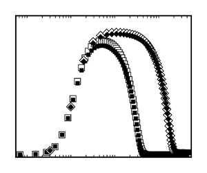
Figure 8 provides a comparison between the DNS data of the Reynolds shear stress and the approximate (2.28). Both the inner scaled wall-normal distance (figure 8a) and the outer scaled wall-normal distance (figure 8b) are used for this comparison. In both plots, the open symbols represent the DNS data, while the filled symbols depict values calculated from the approximate (2.28). The use of log-linear axes in figure 8(a) enhances the visualization of the variation in the Reynolds shear stress and the approximation equation within the near-wall region. The figure demonstrates notable agreement between the approximate equation and the DNS data, with only minor deviations observed for the lowest Reynolds number data.

Figure 8. Comparison of the approximate (2.28) and DNS data. (a) Inner scaled wall-normal distance. (b) Outer scaled wall-normal distance. The open symbols represent the DNS data of the Reynolds shear stress, and the filled symbols represent the approximate equation. Data from SO and SJHM as in figure 1.

The DNS data presented in figure 8 correspond to relatively moderate Reynolds numbers. In order to investigate the influence of Reynolds number on the accuracy of the approximate (2.28), figure 9 showcases experimental data encompassing a broader range of Reynolds numbers. For comparison purposes, the DNS data from Schlatter & Örlü (Reference Schlatter and Örlü2010) at $Re_\tau =974$ are also included in the figure. As expected, the experimental data exhibit larger variability compared to the DNS data. However, despite the increased scatter, the deviation between the measured Reynolds shear stress and the approximate (2.28) remains relatively small and does not demonstrate a distinct dependence on Reynolds number. The larger discrepancy observed in the near-wall region can be attributed to the limited availability of experimental measurements close to the wall. Nevertheless, the overall agreement between the experimental data and the approximate equation suggests that it offers a reasonable estimation of the Reynolds shear stress, especially in the outer region of the boundary layer.

Figure 9. Comparison of the approximate (2.28) with the experimental data from Baidya et al. (Reference Baidya, Philip, Hutchins, Monty and Marusic2021) (B). The DNS data from Schlatter & Örlü (Reference Schlatter and Örlü2010) (SO) at $Re_\tau =974$ are included for reference.

Figures 8 and 9 provide strong evidence supporting the effectiveness of the approximate (2.28) in accurately capturing the distribution of Reynolds shear stress around its peak. In other words, the approximate (2.28) predicts reliably the Reynolds shear stress distribution within the meso-layer region of the four-layer structure proposed by Wei et al. (Reference Wei, Fife, Klewicki and McMurtry2005).