Introduction
One of the main characteristics of the snow cover in mountain regions is its spatial heterogeneity (Reference Sturm and BensonSturm and Benson, 2004). For avalanche formation, spatial variations in snow mechanical properties at the snowpack-depth and slope scale are believed to be crucial for slope stability (for a definition of scales see Reference Schweizer and KronholmSchweizer and Kronholm, 2007). Spatial variations will either promote or hinder avalanche formation, depending on the size and scale of heterogeneity and on the average stability (Reference Kronholm and SchweizerKronholm and Schweizer, 2003). The relevance of spatial variability for avalanche formation stems from the view that the release of a dry-snow slab avalanche is essentially a fracture mechanical process. In fracture mechanics, stability depends on flaw size, among other variables, so that slope stability becomes dependent on the relation between critical flaw size and the scale of heterogeneity (Reference Schweizer, Jamieson and SchneebeliSchweizer and others, 2003a).
Spatial heterogeneity at various scales (snowpack-depth, slope, basin) limits the accuracy of regional avalanche forecasting. Therefore, in order to improve avalanche forecasting, it is essential to quantify spatial variations of snowpack properties in relation to avalanche formation. Snow-stability evaluation for the purpose of avalanche forecasting typically relies on field observations or measurements at representative sites. As sampling cannot be ubiquitous in space and time, extrapolation from point observations (scale: snowpack depth) is required. Spatial variability studies aim, among other things, at quantifying (and eventually predicting) the amount of uncertainty introduced into avalanche forecasting by extrapolation from point measurements (Reference Landry, Birkeland, Hansen, Borkowski, Brown and AspinallLandry and others, 2004).
Point observations are representative for the snowpack depth scale and include the layer scale. The question in the realm of stability evaluation and avalanche forecasting is whether the point observation is representative for the slope scale and whether that particular slope is representative for similar slopes of the same aspect and elevation. A multi-scale approach therefore seems most appropriate for answering these questions. However, collecting multi-scale data requires either significant skilled human resources, which are often not available and might introduce an observational bias, or compromises in spatial resolution that inhibit a geostatistical analysis. It has been proposed that most of the weak layer variation might be caused at the snow surface before burial (Reference Feick, Kronholm and SchweizerFeick and others, 2007). We therefore focused our field observations on the snow surface properties.
Whereas many spatial variability studies have been performed in the past at the slope scale (Reference Birkeland, Kronholm, Schneebeli and PielmeierBirkeland and others 2004; Reference Kronholm, Schneebeli and SchweizerKronholm and others, 2004; Reference Landry, Birkeland, Hansen, Borkowski, Brown and AspinallLandry and others, 2004) and at larger scales (Reference BirkelandBirkeland, 2001; Reference Schweizer, Kronholm and WiesingerSchweizer and others, 2003b), this is to our knowledge one of the first systematic multi-scale studies on snow-cover properties in relation to avalanche formation. For a recent review on spatial variability studies, see Reference Schweizer, Kronholm, Jamieson and BirkelandSchweizer and others (2008).
The aim of the present study is to characterize the surface layers at the snowpack-depth, the slope and the basin scale on the same day, in order to quantify the variations at the different scales and to estimate conditions under which extrapolation seems feasible. Observations were related to meteorological conditions and compared to the simulated snow-cover properties.
Methods
Study site and instrumentation
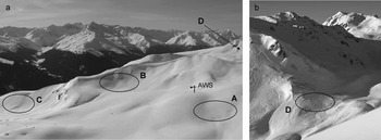
The study site is the Steintälli–Strelapass area above Davos, eastern Swiss Alps (46°48′ N, 9°47′ E). The area is above the tree line and reaches up to about 2600 m a.s.l. Four study slopes were chosen within the drainage that have similar aspect and elevation. They are located between 2300 and 2450 m a.s.l. and their aspect is north to northeast. Slopes A, B and C have similar exposure, not only to the sun but also to the wind. They are fairly sheltered slopes, as much as can exist at all above the tree line. Slope D has similar aspect and elevation, but is located just above a pass and is hence more exposed to wind (Fig. 1).

Fig. 1. The study area above Davos: (a) slopes A, B and C as well as the location of the AWS, with slope D further right and behind; and (b) the more wind-exposed slope D.
As we wanted to compare different slopes on a single day, and as it took about 1–2 hours to complete the observations, we had to focus on a single slope aspect. To avoid diurnal perturbations as much as possible, we chose shady slopes of northerly or northeasterly aspect. In addition, the slopes had to be close together (longest distance between two slopes: 1.25 km) and safe access was important. The slopes themselves had to be fairly safe, i.e. rather small, not too steep (close to 30°), but still potential avalanche slopes. Only slope A was not steep enough to slide. Table 1 summarizes slope characteristics.
Table 1. Characteristics of study slopes. Slope exposure to wind was qualitatively assessed based on the distance to the next major ridge

About 50 m south of slope A, and 300 m northwest of slope B, an automatic weather station (AWS) was located on a small knoll. Measurements every 10 min include air temperature (not ventilated), snow surface temperature (infrared sensor), horizontal wind speed and direction (propeller-type anemometer), relative humidity (capacitive measurement), incoming and reflected shortwave radiation and net radiation balance.
Field observations
The observations were a combination of snow micro-penetrometer (SMP) measurements (Reference Schneebeli, Pielmeier and JohnsonSchneebeli and others, 1999) and manual characterization of the snow cover. The design was chosen such that the snowpack depth scale, the slope scale and the basin scale could be covered in 1 day (Fig. 2). On each slope, observations were made at five locations (1–5): in the corners and the middle of a 10 m × 10 m square. At each of the five locations, four SMP measurements were done in the corners of a small 1 m × 1 m square. In the middle of the small squares the snow surface layer was characterized manually (grain type and size, hand hardness index and surface roughness) according to the International Classification for Seasonal Snow on the Ground (ICSSG) (Reference ColbeckColbeck and others, 1990). Apart from the surface-roughness classes defined in the ICSSG, we used the term rough to describe snow surfaces that were generally smooth but had small-scale (5–10 mm) surface roughness. In addition, the snow surface was photographed. In the middle of the 10 m × 10 m square, a full manual snow profile (grain type and size, snow hardness index, density and snow temperature) was usually taken for the topmost metre and a stability test (compression test: CT) (Reference JamiesonJamieson, 1999) was performed. Below we do not report on the latter two types of measurements but focus on surface properties.
Fig. 2. Sampling design showing the multi-scale approach that attempts to cover the snowpack, the slope and the basin scale. Circles (O) denote locations of SMP measurements, ‘M’ of manual observations of surface characteristics and ‘P’ is profile location.
With a maximal extent of ∼15 m we only covered a relatively small part of the slopes, but this was required in order to enable repeated measurements on the same slope. The two measurement methods have different support (i.e. area or volume over which each measurement is integrated), i.e. 2 × 10⁻⁵ m2 (SMP) and ∼0.1 m2 (manual characterization) (Reference Blöschl and SivapalanBlöschl and Sivapalan, 1995).
Snow-cover simulation
Snow-cover stratigraphy and its evolution was simulated for the location of the AWS with the numerical snow-cover model SNOWPACK (Reference Bartelt and LehningBartelt and Lehning, 2002; Reference Lehning, Bartelt, Brown, Fierz and SatyawaliLehning and others, 2002a, Reference Lehning, Bartelt, Brown and Fierzb). For the analysis we compared simulated snow surface characteristics (grain shape and size of the topmost layer) with observed characteristics.
Data analysis
To describe and compare surface properties, the penetration resistance of the topmost layer was analyzed. The layer boundary was delineated manually (Reference KronholmKronholm, 2004). Alternatively, simply the topmost 2 cm were defined as the surface layer. Below, only the analysis for the topmost 2 cm is presented. Robust (non-parametric) measures such as the median and the quartile coefficient of variation (QCV) were used to describe the penetration resistance in the topmost 2 cm which were sampled every 4 μm.
The data from within and between scales were compared using the non-parametric Kruskal–Wallis test (H-test) (non-spatial analysis). A level of significance p = 0.05 was chosen to decide whether the observed differences were statistically significant. As at the snowpack-depth scale only four measurements were available, no real statistical analysis was possible. Nevertheless, we tried to express in a quantitative way how different the four measurements were compared to the typical standard error (SE). For that purpose we determined the 95% confidence interval (CI = 1.96SE) for all measurements on a given slope. Relative to the slope mean penetration resistance of all measurements, the 95%CI varied for the four slopes between 18 and 27%, with an average of 23.5%. We then simply checked whether measurements were within the confidence limits (±23.5% of the median penetration resistance at that point) and assumed that if this was the case, the measurement was considered similar to the others. If all four measurements were within this range the small-scale, that is, the snowpack depth-scale, variability of the surface hardness was considered rather small. Alternatively, if all four measurements were outside the range, this indicated strong small-scale variations.
Explicit spatial analysis was made using the semivariogram. The semivariogram γ(h) estimates the variance at increasing intervals of lag distance h between measurement locations. It is a spatial dissimilarity measure and is mainly used to assess whether spatial data are autocorrelated. We first transformed the SMP data to bring the distribution closer to normality (log10 transformation), removed the slope-scale trend (linear model), used a robust method to calculate the sample variogram and then fitted a spherical model to the data. The procedure is described in detail by Reference Kronholm, Schneebeli and SchweizerKronholm and others (2004).
Simulated and manually observed snow surface layer characteristics were compared using the PROFEVAL comparison routine as described by Reference Lehning, Fierz and LundyLehning and others (2001). The method provides a distance measure that describes the agreement between observation and/or simulation. The method was applied to objectively assess differences in grain shape and grain size between observation sites as well as between observation and simulation. The measure (relative distance) varies between 0 (perfect agreement) and 1 (no agreement). The separately calculated distance measures for grain size and shape were combined such that the un-weighted average is given.
Data
Observations were made on 16 days from January to March 2004 (Table 2). Due to poor weather, critical avalanche conditions or technical problems, not all four slopes could be covered on each of these days. Eventually, only on two days were SMP data for all four slopes available for analysis; on seven days data for at least three slopes, and on two more days data for two slopes could be analyzed. Manual observations were available for all 16 measurement days and slopes that were vizited on that day. In addition, on each day surface characteristics were observed at the AWS. On the slopes, full snow profile observations of the uppermost metre of the snow cover started in early February 2004. At the AWS, five full snow profiles were made during the observation period from January to March 2004.
Table 2. Compilation of measurement days and data. A–D denotes the four study slopes (see Table 1). If SMP data were acquired this is denoted with ‘x’; with ‘(x)’ if the data were not usable for analysis. If the slope was not visited, this is marked with ‘O’. In the two last columns the number of manual profiles per day and the number of days since the last snowfall are given

The 2003/04 winter was an above-average snow year. During our observation period, it snowed frequently, almost all days in January and during the second week of February. There were some periods of sunny and calm weather in early and mid-February, and at the end of February to the beginning of March. Accordingly, our measurement days are often after a storm, but occasionally between storms.
Results
Before we compare the data from the four slopes for selected days, we present the penetration resistance for the whole observation period (Fig. 3). The penetration resistance in the top 2 cm of the snowpack for slopes A, B and C was not significantly different (p = 0.69), ∼0.02 N, whereas it was about an order of magnitude higher for slope D. The standard errors were ∼0.0028 N, 0.0056 N, 0.0055 N and 0.03 N for slopes A–D, respectively. These values are fairly low compared to the noise of the instrument in air, which is ∼0.01 N. The above seasonal comparison, which implies comparing the different sites on different days, is generally not appropriate for finding differences between the slopes since there could be completely different conditions between slopes on different days that average out over the winter. However, a seasonal comparison is useful to assess the overall range of variation.

Fig. 3. Penetration resistance of the topmost 2 cm of the snowpack for slopes A–D. All data from the 11 measurement days are shown to provide a measure of the range of variation during winter. Boxes span the interquartile range from first to third quartile, with a horizontal line showing the median. Notches at the median indicate the confidence interval (p < 0.05). Whiskers show the range of observed values that fall within 1.5 times the interquartile range above and below the interquartile range. Asterisks denote outside values. The number of measurements is N = 236, 210, 183 and 79, for slopes A–D, respectively.
Non-spatial analysis
We first present the non-spatial results at the snowpackdepth, slope and basin scale. Only the results from three selected days are presented in detail. The observations on two days (8 January and 13 February 2004) were shortly after a snowfall, whereas the observations on 17 February 2004 were after 4 days without precipitation.
8 January 2004
Figure 4 shows the penetration resistance on 8 January 2004 of the top 2 cm over the four slopes. On the days before 8 January 2004, it snowed about 5–10 cm d−1. The snow surface was manually characterized, consistently for the slopes A, B and C, as a mixture of graupel and small crystals of surface hoar ∼1–2 mm in size (Table 3). The surface was either smooth or slightly rough (some random furrows due to wind). On slope D, however, the snow surface was considerably wind-affected and sastrugi were present. Accordingly, the dominant snow crystal types were small rounds and decomposed and fragmented particles with occasional small surface hoar.

Fig. 4. Penetration resistance of the topmost 2 cm for slopes A–D on 8 January 2004 (top row), 13 February 2004 (middle row) and 17 February 2004 (bottom row). Whereas on the left all measurements on a slope are given (slope scale), on the right the measurements are shown per point (snowpack depth scale); small figures indicate how many measurements per point were outside of the confidence interval. Same figure type as shown in Figure 2 (with circles denoting far outside values).
Table 3. Results of manual observations on slopes A–D on 8 January 2004, 13 February 2004 and 17 February 2004. Grain type and grain size (in mm) are given according to the ICSSG (Reference ColbeckColbeck and others, 1990). n/a: not applicable

At the snowpack-depth scale, the measurements at the four corners of the small 1 m × 1 m square were compared. A geostatistical analysis is not possible. For 8 January 2004, in 11 out of 20 cases, at least three out of four measurements within the square were similar, i.e. fell within the range of ±23.5% of the median of the four measurements (Fig. 4). Slope B (Steintälli) had the strongest small-scale variations. Also, none of the medians of the snowpack depth-scale measurements fell within the range ±23.5% of the slope median. This means that there were considerable differences between the five snowpack depth-scale measurement locations on slope B. On slopes A, C and D, the small-scale variation within as well as between the measurement points was lower than on slope B. For example, on slopes A and C, all five median values of the snowpack depth-scale measurements fell within the slope-scale median.
Slopes A–C had fairly similar (though increasing from A to C) penetration resistance, i.e. very low values between 0.019 N and 0.032 N were measured (Fig. 4). However, the H-test (p < 0.001) indicates that the three slopes were significantly different. Since the penetration resistance over slope D was about ten times larger than for slope A, the four slopes were considered as statistically different (H-test, p < 0.001). Only the samples from slopes A and B were considered as statistically not different (p = 0.29). However, the QCV (Table 4) was very similar for slopes A (15%), C (19.5%) and D (19%), which confirms the above observation that the variation within the 10 m × 10 m square, at the slope scale, was similar.
Table 4. Medians and quartile coefficients of variation (QCV) of (not-transformed) penetration resistance (topmost 2 cm) at the slope scale (N = 20, occasionally only 18 or 19 measurements). A–D denote the study slopes. n/a: not applicable

13 February 2004
The observations on 13 February 2004 followed an extended snowfall period. The snow surface consistently comprised small rounds mixed with graupel of size 0.25–1 mm (Table 3). The snow surface was slightly wind-affected. A thin (1–3 mm) but very soft wind crust was observed. Due to the graupel the surface roughness was classified as rough (not as smooth).
The penetration resistance of the topmost 2 cm of the snowpack was consistently very low (<0.1 N) on all slopes. Slopes A and B showed little variation at the snowpack depth scale. On slope C, at two points (P2 and P3), the variations were large at the snowpack depth scale (Fig. 4). Slope D was not vited on that day. At the slope scale, slope B showed the lowest variation, whereas slope C was fairly variable, with four medians from the point measurements outside the ±23.5% range of the slope median. Slopes A and B had the lowest QCVs of all slopes observed during this study (Table 4). Despite very similar snow surface characteristics, the slope medians of the penetration resistance (topmost 2 cm) were different (0.024 N, 0.031 N and 0.012 N, for slopes A, B and C, respectively), so that the non-parametric H-test indicated that the three slopes were significantly different (p < 0.001).
17 February 2004
A few days later, on 17 February 2004, all four slopes were visited. Surface hoar had formed and was consistently observed on slopes A–C (Table 3). Its size (∼2–5 mm) was almost uniform over the slopes. However, on slope D, the surface hoar had been destroyed and there were sastrugi. In the lee of the sastrugi, small surface hoar was found, whereas on the windward side facets were observed.
The penetration resistance of the topmost 2 cm of the snowpack was still very low (<0.1 N), but had slightly increased since the measurements on 13 February 2004. Slopes A and B showed considerably more variation at the snowpack depth scale (Fig. 4) than 4 days previously. Slope D had large snowpack depth-scale variations due to the existence of sastrugi. Also, at the slope scale, only two (out of five) medians of the snowpack depth-scale measurements fell within the range ±23.5% of the slope median, resulting in a large QCV (56.1%). Based on the H-test, slopes A, B and D were judged as being from the same population (p = 0.07), i.e. there was no statistically significant difference between these slopes.
All days
Figure 5 and Table 4 confirm that on most days, not only on the three days described above in detail, slopes A–C had similarly low surface hardness (though the slopes had significantly different penetration resistance), whereas the snow surface was typically harder on slope D. Comparing all days, when all the sites being compared have been sampled, the median penetration resistance on slopes A, B and C was not significantly different (p = 0.20), whereas if all slopes were considered, a significant difference was found (p < 0.001). The QCVs were 23, 24, 32 and 55% for slopes A–D, respectively. QCVs were not significantly different between slopes A, B and C (p = 0.21), but there was clearly an increasing trend from A and B to C to D.

Fig. 5. Penetration resistance of the topmost 2 cm for slopes A–D. All observation days with SMP data are shown. Same figure type as shown in Figure 2.
Manual surface characterization
Comparison of grain shape and size based on the relative distance measure showed that differences within slopes were generally small, i.e. in most cases <0.1 for slopes A–C, and somewhat higher (∼0.2) on slope D (Fig. 6a). Overall, the differences within slopes were similarly small on all slopes (p = 0.77). The differences between slopes were obviously larger, but still small. Slope D had significantly larger differences to its neighbouring slopes than slopes A–C (p = 0.04) (Fig. 6b). To assess the representativity of the location of the AWS for the study slopes, the differences between the manual observation at the AWS and the slopes were calculated. The relative distances were comparable to the distances within the slopes (Fig. 6c). Again, the distance was largest to slope D. Finally, the simulated grain type and size of the snow surface layer was compared to the observation at the AWS. The difference was found to be fairly large (∼0.55).

Fig. 6. Median differences in manual observation of snow surface (grain shape and size): (a) within slopes (A–D); (b) between slopes; and (c) between the automatic weather station (AWS) and the slopes, and the snow-cover model SNOWPACK (SNP), respectively. The differences are normalized and vary between 0 (complete agreement) and 1 (no agreement). The number of comparisons N is given in (c). Same figure type as shown in Figure 2.
In general, the relative distance was larger for grain size than for grain type. This difference is mainly due to the different data type (categorical vs numerical) and its resolution: whereas the grain size might differ, the grain type is still rather similar and falls into the same category.
Spatial analysis
The results of the geostatistical analysis using the semivariogram are summarized in Table 5. After transformation and removing the slope-scale trend (which in only two cases was statistically significant), for 13 slopes (out of 33) spatial autocorrelation between the points where the penetration resistance of the topmost 2 cm had been measured was found, i.e. a range (<15 m) could be determined. For 19 slopes no range was found or the analysis suggested a range of 0 m – which can be considered as about an equivalent result. For one slope the variation still increased within the extent suggesting a range >15 m. If a range of autocorrelation was found it was in most cases ∼6–11 m.
Table 5. Results of geostatistical analysis of (log10-transformed) penetration resistance at the slope scale (after removal of linear slope-scale trend). Nugget, sill and range of the modelled semivariogram are given. n/a: not applicable

Figure 7 shows the semivariograms for 8 January 2004. On slope D (and likewise on slope C) there was no range found as it was not possible to fit a reasonable model vario-gram to the data. The range on slope A was found to be ∼10 m, and on slope B ∼5 m. On slopes C and D the variance did not increase with increasing distance, at least not within our measurement extent (∼15 m). The total sill was relatively low, in particular when compared with slopes A and B. On that day the non-spatial analysis showed that the variations (in terms of QCV) were largest on slope B and similar on slopes A, C and D. This suggests that there might be a relation between non-spatial variation and the results of the spatial analysis.

Fig. 7. Sample (open circles) and spherical model (line) variograms of penetration resistance (topmost 2 cm) for slopes A–D on 8 January 2004. The median number of point pairs is ∼20.
For 13 February 2004, when the variation was generally small, the spatial analysis revealed no range and very low total sill. On 17 February 2004, when surface hoar was consistently found on slopes A–C, and sastrugi on slope D, the spatial analysis suggested no range for slopes A–C, and a range of ∼5–6 m for slope D. However, relating the QCV of all days and slopes to the corresponding range found in the geostatistical analysis did not reveal any statistically significant relation, in other words the above-mentioned hypothetical relation could not be proved.
Figure 8 shows the basin-scale analysis for the same days that are described in detail above. On 8 January 2004, a range of ∼200 m was found. This is in agreement with the non-spatial analysis that showed, at least in respect to slope A, that the median penetration resistance increased with increasing distance from slope A. On the other two days the variance still increased with increasing distance without reaching a sill. However, the nugget was similar in all three cases (∼0.1–0.2 log N 2). Based on Table 5 it is suggested that the nugget on a sheltered slope is ∼0.05 log N 2, which should about correspond to the measurement error. The analysis at the slope and basin scale confirms that the range of autocorrelation depends on the scale analyzed (Reference BlöschlBlöschl, 1999; Reference Schweizer and KronholmSchweizer and Kronholm, 2007).

Fig. 8. Sample (open circles) and model (line) variograms at the basin scale including all slopes for 8 January, 13 and 17 February 2004. The median number of point pairs is >300.
Causes of variability
We related median penetration resistance, as well as the QCV and the range of autocorrelation, to meteorological parameters measured at the AWS. These weather parameters included new-snow depth (24 hours), average wind speed (24 hours), average maximum 10 min wind speed (24 hours), maximum gust (24 hours), standard deviation of 10 min maximum wind speed (a potential measure of turbulence), air temperature at noon the previous day, and number of days since the last snowfall. None of these parameters was significantly correlated with the surface hardness or its variations. The median penetration resistance on slopes A and B, which are closest to the AWS, were weakly related to the new-snow depth (negatively) and the number of days since the last snowfall (positively). In fact, when grouping the observation days into days immediately after a storm, and days after some precipitation-free days, the median penetration resistance of the topmost 2 cm was significantly lower for the storm days than for the calm days (p = 0.015). Three (A, B and D) out of four slopes had lower QCV after a snowfall and higher after some days without precipitation (H-test not significant).
Summary and Conclusions
We measured and observed the surface characteristics at the snowpack-depth, the slope and the basin scale. During the 2003/04 winter we regularly visited up to four shady slopes in the vicinity of an AWS. Three slopes were fairly sheltered, and one was strongly exposed to wind. We focused on snow surface properties as those seem to be crucial for avalanche formation (bonding to subsequent snowfall).
A particular methodological difficulty was to objectively determine the level of variability. Different methods revealed different results, mainly depending on the measurement support (the area or volume over which each measurement is integrated) (Reference Blöschl and SivapalanBlöschl and Sivapalan, 1995) and the accuracy of the method.
At the snowpack depth scale, typically, in about half of the cases, at least three measurements were within the confidence limits we defined (median ±23.5%) to assess the representativity at the snowpack depth scale. Otherwise, large variations were observed at the snowpack depth scale in terms of penetration resistance in the topmost 2 cm. Similarly large variations at snowpack depth scale were found by Reference Landry, Birkeland, Hansen, Borkowski, Brown and AspinallLandry and others (2004). On the other hand, the manual observations indicated a low degree of heterogeneity, in particular on the more sheltered slopes, but even, to a lesser degree, on the wind-exposed slope. In other words, the relative variation at the snowpack depth scale was not as different as expected between the more sheltered and the wind-exposed slopes.
At the slope scale, the variability was often determined by the variability at the snowpack depth scale. For example, large variations at the snowpack depth scale on slope D caused large variations at the slope scale, i.e. QCV≈50%. Within slopes variations varied between observation days, but were typically rather low (QCV≈25–30%) for the three sheltered slopes and high for the wind-exposed slope. Slope-scale variations on the order of 25–50% have also been found in previous studies using the SMP (e.g. Reference KronholmKronholm, 2004). Studies conducted with stability tests typically found less variation due to the higher support (e.g. Reference Landry, Birkeland, Hansen, Borkowski, Brown and AspinallLandry and others, 2004). If penetration resistance is considered, QCV≤25% represents rather low variability. This was the case on almost half of the slopes we tested (Table 4).
At the basin scale, substantial differences between the slopes were observed. Whereas slopes A and B that were closest together had fairly similar slope-scale variations, the variation was larger for slope C and again for slope D. Slope D showed the largest snowpack depth-scale variation and also differed most in median penetration resistance of the surface layer (topmost 2 cm). However, overall, the variation between the sheltered slopes was similar, in terms of penetration resistance (median penetration resistance and QCV) as well as in regard to grain shape and size (Fig. 6b). The three wind-sheltered slopes can be considered as representative of each other – despite some significant differences on some days. On almost all days the penetration resistance was consistently low (≤0.1 N) (Fig. 5). The wind-exposed slope D was significantly different from the other slopes and had generally higher penetration resistance. According to Reference Pielmeier and SchneebeliPielmeier and Schneebeli (2003), a penetration resistance of ∼0.1 N corresponds approximately to a hand hardness index of 1 (‘fist’) (ICSSG; see Reference ColbeckColbeck and others, 1990). In other words, considering the hand hardness index, slopes A, B and C had similar surface hardness.
The geostatistical analysis was not conclusive in regard to wind exposure of the slopes or prevailing meteorological conditions. In about one-third of the cases, the analysis suggested that the penetration resistance of the topmost 2 cm was spatially autocorrelated within the measurement extent. In most cases, the penetration resistance did not increase with increasing distance, i.e. measurements within the 10 m × 10 m square were not autocorrelated, hence a range cannot be defined. This result is in agreement with previous studies at the slope scale that also showed that in some cases typical weak-layer properties were autocorrelated while in other cases they were not (e.g. Reference Birkeland, Kronholm, Schneebeli and PielmeierBirkeland and others, 2004; Reference Kronholm, Schneebeli and SchweizerKronholm and others, 2004). The reasons for either the existence or the lack of autocorrelation are not clear but probably associated with the layer-deposition pattern and the subsequent changes to the layer when buried (Reference Schweizer, Kronholm, Jamieson and BirkelandSchweizer and others, 2008). Despite the lack of spatial structure, the measurements at the slope scale might still be representative of each other (e.g. slope C on 8 January 2004), depending on the slope-scale variation which varied considerably between observation days.
The analysis of the causes of variability at the slope scale was mainly not conclusive. None of the weather parameters considered was related to either the penetration resistance, its variation at the slope scale or the range. This suggests that basin-scale meteorological conditions, as measured with an AWS located at a representative site, might not suffice to explain sub-scale features. However, in the present case, it was shown that the AWS seems to be representative of the sheltered, shady slopes A–C, at least in regard to grain shape and size (Fig. 6c). The slope- and sub-slope-scale variations might be due to local weather phenomena that are not captured by the AWS.
However, there was a general trend to lower penetration resistance in the topmost 2 cm and lower slope-scale variation after a snowfall event and higher resistance and variability during a subsequent period of fair weather. This observation is in agreement with the hypothesis by Reference Birkeland, Landry and StevensBirkeland and Landry (2002) that spatial variability at the slope scale generally increases through time, except in the presence of some sort of external forcing (e.g. precipitation) when instead it might decrease.
As mentioned above, there was good agreement between snow surface characteristics at the location of the AWS and the sheltered slopes. This suggests that the AWS is apparently in a good location and the data should be useful for avalanche forecasting. In particular, numerical simulation of snow stratigraphy and therefore of derived stability for the location of the AWS might be useful for regional-scale avalanche forecasting (Reference Schweizer, Bellaire, Fierz, Lehning and PielmeierSchweizer and others, 2006). However, to support this, a more comprehensive comparison between the snow stratigraphy on the slopes and the observed and simulated snow stratigraphy at the flat location of the AWS would be required (Reference Fierz and GauerFierz and Gauer, 1998). The comparison of snow surface characteristics between manual observations and simulations at the location of the AWS was not yet satisfactory, suggesting that the usefulness of snow-cover simulation for avalanche forecasting is still limited.
We have shown that snow surface characteristics and their variation vary depending on slope exposure to wind and to some degree on general weather conditions. Similar slopes in terms of exposure showed similar spatial variability, and extrapolation seems possible. However, this conclusion depends on the method applied. We have compared two methods with different support that clearly revealed different results in regard to spatial variability. Whereas the fine-resolution, small-support SMP measurements in most cases suggested significant variability, the manual observations indicated very limited variability. It is unclear whether the amount of variation found by the SMP is already relevant for avalanche formation. The general problem in regard to avalanche formation is to define the relevant level of spatial variability.
In summary, the multi-scale study revealed various degrees of variability. The variations were largest whenever the snowpack was wind-affected. Whereas this finding can be, depending on the scale, favourable or unfavourable for avalanche formation, it definitely represents a challenge for numerical simulation of snow-cover stratigraphy and therefore of derived stability prediction.
Acknowledgements
We thank R. Dadic for help with the field observations and K. Kronholm and M. Schneebeli for valuable discussions. The comments by Chief Editor T.H. Jacka and two anonymous reviewers helped to significantly improve the paper and were much appreciated.