


INTRODUCTION
Time series of remote-sensing images from passive microwave scatterometer sensors are used in snow-melt detection and measurement in the Antarctic continent (Liu and others, Reference Liu, Wang and Jezek2006; Tedesco, Reference Tedesco2009; Trusel and others, Reference Trusel, Frey and Das2012; Barrand and others, Reference Barrand2013) and other cryosphere areas (Fettweis and others, Reference Fettweis, Tedesco, van den Broeke and Ettema2011), and for mapping the Antarctic surface mass balance (Magand and others, Reference Magand, Picard, Brucker, Fily and Genthon2008) and several studies involving remote sensing of the cryosphere. Traditional snow-melt detection applications (Liu and others, Reference Liu, Wang and Jezek2006; Tedesco, Reference Tedesco2009; Fettweis and others, Reference Fettweis, Tedesco, van den Broeke and Ettema2011; Trusel and others, Reference Trusel, Frey and Das2012; Barrand and others, Reference Barrand2013) are based on Boolean approaches and detect snow melt in the image pixels using wavelet analysis methods that allow spatial analysis of snow-melt patterns and trends in the Antarctic continent. A different approach based on the subpixel analysis for estimation of snow melt at the Antarctic Peninsula using microwave passive time-series images was proposed by Mendes-Júnior (Reference Mendes-Júnior2010) based on spectral linear mixing models (SLMM) for generation of fraction images of three endmembers, namely, wet snow, dry snow and rock outcrops. This subpixel analysis approach applied for snow-melt detection is based on the methodology developed by Haertel and Shimabukuro (Reference Haertel and Shimabukuro2005), which adopts higher spatial resolution images for calculation of the endmember spectral signatures.
This paper reports a comparative analysis on fraction-image time series of the Antarctic Peninsula for the period 1999–2009, as generated by multiresolution remote-sensing images (SSM/I and SSMI/S with 25 km and QuikSCAT with 2.225 km of spatial resolution) for snow-melt detection. The comparative analysis is based on: (a) performance evaluation of the wet-snow fraction images using classified images from higher spatial resolution data (ASAR with a 75 m of spatial resolution) for 11 dates and (b) comparative analysis of melt metrics (melt area extent and melt index) derived from a subpixel analysis based on data from the literature (Trusel and others, Reference Trusel, Frey and Das2012).
STUDY AREA AND DATA
Study area
The Antarctic Peninsula (Fig. 1) is one of the areas most affected by climate change in the Antarctic region. This area covers 522 000 km2 with an average elevation of 1500 m (Bindschadler, Reference Bindschadler2006) from 62.5° to 73°S. The focus of this study is land and permanent ice shelves located in the continental area of the Antarctic Peninsula, i.e. sea-ice and temporary ice shelves were not accounted in this study.
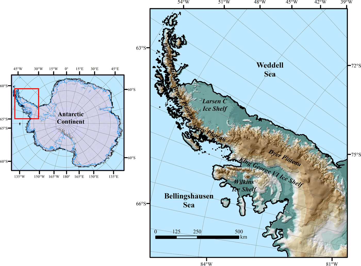
Fig. 1. Localization map of the Antarctic Peninsula.
Advanced Synthetic Aperture Radar (ASAR)
The ASAR instrument onboard the ENVISAT satellite and operating on the C-band (5.6 cm) ensures continuity of the ERS-1/2 AMI data and features enhanced capabilities in terms of coverage, range of incidence angles, polarization, and imaging modes. In this study, we used ASAR WS (Wideswath mode) from 2006 to 2008 with a spatial resolution of ~ 56 m (resampled to 75 m) and varying temporal resolution according to the imaging mode. The ASAR images were used in this study as a baseline for high-spatial-resolution data for estimation of the spectral signatures (endmembers) of the SLMM and validation of the wet-snow fraction images.
SSMI
Microwave time-series images that measure the brightness temperature (T b) of SSMR, SSM/I, and SSMI/S sensors from 1978 to the present are available for Antarctic ice cover. We used F11 and F13 SSM/I and F17 SSMI/S EASE-Grid data from the 19H, 19 V, 37H, and 37 V channels from 1999 to 2009 with a spatial resolution of ~25 km and a daily temporal resolution. These data are available to the general public for download at the National Snow and Ice Data Center NSIDC (http://nsidc.org/data/NSIDC-0032). Despite the low spatial resolution, the SSMI data are important for melt detection globally due to the daily temporal resolution and historical imaging.
QuikSCAT
QuikSCAT scatterometer backscattering (σ 0) image data generated by the BYU Center for Remote Sensing (CERS) are available for download (http://www.scp.byu.edu) with daily resolution for the Antarctic continent in the 1999–2009 period. QuikSCAT images are generated from the SeaWinds on QuikSCAT egg backscatter measurements and from the slice measurements with nominal spatial resolutions of 4.45 and 2.25 km, respectively. In this study, we used slice images reconstructed from mid-day orbit passes at the horizontal (qnsh) and vertical (qnsv) polarizations by applying the Scatterometer Image Reconstruction with Filtering (SIRF) algorithm (Early and Long, Reference Early and Long2001).
METHODS
The methodology used in this work (Fig. 2) applies the following steps: (a) preprocessing of multitemporal remote-sensing data, (b) subpixel mixture analysis of SSMI and QuikSCAT time-series images from the years 1999–2009, and (c) evaluation of subpixel analysis-based wet-snow fraction-image time series, including assessment of fraction images by independent ASAR dataset and sensitivity analysis of the melt metrics measured with wet-snow fraction images.
Fig. 2. Methodological approach adopted in this work.
Preprocessing of remote-sensing data
Initially, we performed selected pre-processing on the ASAR (radiometric and geometric calibration and multitemporal classification) and SSMI (calibration and space–time filtering) images.
Calibration and multitemporal classification of ASAR images
The multitemporal classification of ASAR images (the dataset with the highest spatial resolution in this study) was based on a decision tree approach and was performed on 16 images (from 2006 to 2008) used to estimate the SLMM spectral signatures and on an independent dataset (12 images from 2006 to 2008) used to validate the SLMM wet-snow fraction-image results. The classes defined in this study were wet snow, dry snow, and rock outcrops.
The original 1P level ASAR WS images were subjected to antenna-related radiometric calibration before performing (a) radiometric calibration for calculation of the backscattering coefficients based on the algorithm developed by Laur and others (Reference Laur2002), (b) speckle filtering by adopting a median 5 × 5 moving window, and (c) orthorectification using the Landsat TM mosaic as geospatial reference data and the RAMP DEM as the topographic information.
The decision trees rules for ASAR image classification (Arigony-Neto and others, Reference Arigony-Neto2007, Reference Arigony-Neto2009) were built based on backscattering thresholds determined by Rau and others (Reference Rau, Braun, Friedrich, Weber and Goßmann2000), information found in the literature for the altitudinal distribution of glacier facies on the Antarctic Peninsula (Simões and others, Reference Simões, Bremer, Aquino and Ferron1999; Braun and others, Reference Braun, Rau, Saurer and Goßmann2000; Rau and others, Reference Rau, Braun, Friedrich, Weber and Goßmann2000; Skvarca and others, Reference Skvarca, De Angelis and Ermolin2004), and the image ratio of summer and winter σ 0 images for discriminating between wet and dry-snow zones. Using a snow backscatter model in the C-band, Rau and others (Reference Rau, Braun, Friedrich, Weber and Goßmann2000) validated the empirically derived thresholds for backscattering used in classification of radar glacier zones in the Antarctic Peninsula. The difference in areas with the occurrence of the dry-snow zone in the northern (1200 m) and the southern (800 m) portions of the peninsula (Rau and Braun, Reference Rau and Braun2002) determined using the RAMP DEM was used as a threshold to mask sectors where we did not expect to find pixels classified as wet-snow. The rock outcrops were classified using a mask based on the SCAR Antarctic Digital Database (ADD) data. Finally, the classification results were post-processed using a focal majority analysis with a 5 × 5 moving window.
Calibration and space–time filtering of SSM/I and SSMI/S images
For time-series analysis, the T b from these sensors should be recalibrated. Using the F8 SSM/I data as a baseline, we can convert the SMMR, F11 SSM/I, and F13 SSM/I data into F8 SSM/I equivalent responses using the regression coefficients derived by Jezek and others (Reference Jezek, Merry and Cavalieri1993) and Abdalati and others (Reference Abdalati, Steffen, Otto and Jezek1995). For radiometric calibration of SSMI/S images, we applied the linear regression coefficients proposed by Abdalati and others (Reference Abdalati, Steffen, Otto and Jezek1995) for the four channels 19H (intercept=−1.17 and coefficient= 1.008), 19 V (intercept=−0.932, and coefficient=1.002), 37H (intercept=−3.59 and coefficient=1.019), and 37 V (intercept=−2.23 and coefficient=1.008).
For calibration of the F17 SSMI/S data, we estimated the linear regression coefficients by models with R 2 >0.98 using F13 SSM/I pre-calibrated data as reference. The model parameters for the intercept and regression coefficient were, respectively, −0.394 and 1.015 (19H), −1.269 and 1.016 (19 V), 3.446 and 0.979 (37H), and 1.185 and 0.989 (37 V). All of the model coefficients were statistically significant (p-value <0.0001).
For suppression of bad data pixels due to noisy signals or missing SSMI data, the days without images were completely interpolated using the mean of the previous and subsequent imaged days. The bad data pixels were interpolated using the average from the 2 to 6 nearest dates with valid T b measures according to an iterative algorithm: (a) first, the interpolation of the bad pixels with the nearest 2 days, (b) second, the interpolation of the remaining bad pixels with the nearest 3 days, (c) third, the interpolation of the remaining bad pixels with the nearest 4 days and so on until 6 days at the maximum.
Subpixel mixture analysis
For estimation of the snow melting according to the wet-snow fraction images, we applied a SLMM, including the three endmembers: wet-snow, dry-snow, and rock outcrops. In this SLMM, the signal (T b in SSM/IS and SSM/I, σ 0 in QuikSCAT) of each pixel in a given sensor channel is the result of a linear combination of each endmember in the sensor IFOV (instantaneous field of view). The contribution of each endmember is weighted by the fraction area of this component at each pixel, and if the endmember signal response is known, Eqn (1) can be used to estimate the fraction of each endmember:
 $$ R_{i, k} = \sum_{\,j=1}^{m} f_{i,j} r_{\,j,k} + e_{i,k}, $$
where R i,k is the average signal response of a pixel i at channel k, f i,j is the fraction of pixel i covered by endmember j, r j,k is the signal response of endmember j at channel k, e i,k error of a pixel i at channel k, j is the number of endmembers (1, 2,…, m) and k is the number of channels (1, 2,…, p). The fraction f j estimates are subjected to the following restrictions:
 $$ \eqalign{ & \sum_{\,j=1}^{m} f_{\,j} = 1, \cr & f_{\,j} \ge 0 } $$
to solve the linear equations system by applying the least-squares fitting to the estimation of f i,j and minimizing the square sum of residuals e i,k, subjected to the above restrictions and the number of pixels n > m and m ≤ p + 1 (Shimabukuro and Smith, Reference Shimabukuro and Smith1991).
Fraction images obtained from sensors with high spatial resolution can be used to estimate the spectral signatures of pure pixels from low spatial resolution sensors (Haertel and Shimabukuro, Reference Haertel and Shimabukuro2005). Because the pixel average spectral response of the channels in the low spatial resolution image is known, the fraction images (f i,j) generated by this process can be applied to estimate the multispectral response of the pure pixels of each endmember (r j,k). In matrix notation, the least square fitting with restrictions for determination of the unknown spectral response (Haertel and Shimabukuro, Reference Haertel and Shimabukuro2005) can be expressed using Eqn (3):
 $$ r_{k} = (F^{T} F) ^{-1} F^{T} R_{k}, $$
where r k is the m-dimensional vector of the endmember spectral response at channel k, F is the fractions n × m matrix, F T is the fractions n × m transpose matrix and R k is the n-dimensional vector of the pixel spectral response at channel k.
We estimated the spectral signatures (endmembers of wet snow, dry snow, and rock outcrops of the SLMM) from the ASAR images (75 m) classified using these 3 classes via a down-scaling approach using zonal statistics with F13 SSM/I (25 km) and QuikSCAT (2.25 km) images from the same acquisition period (16 days from 2006 to 2008). This approach allowed us to apply the Eqn (1) with the f i,j measured from the ASAR fraction images, representing the proportion between the sum of pixels in the ASAR classified image for each endmember and the total number of pixels of the ASAR image composed of 1 pixel of SSM/I and the QuikSCAT images for each band.
Evaluation of subpixel analysis based on wet-snow fraction-image time series
We evaluated the wet-snow fraction-image time series of the SSMI/S and QuikSCAT data using two methods applied twice to these two different data sources: (a) comparison of the fraction images with an independent ASAR classified image dataset of 11 mosaic days from the years 2006, 2007, and 2008, and (b) analysis of the melt detection metrics estimated from the fraction-image time series of SSMI/S and QuikSCAT with respect to other estimates for the 1999–2009 period in the Antarctic Peninsula.
For the assessment of the fraction image and estimation of the melt metric with SSMI and QuikSCAT data, we considered only the continental pixels of the Antarctic Peninsula by applying a mask based on the high-resolution coastline from the SCAR ADD (version 7) (available at http://www.add.scar.org). In the QuikSCAT data, we observed the spatiotemporal persistence (over all the specified years and seasons) of medium-to-high wet-snow fractions (>0.1) in regions with low potential for snow melt (i.e. continental and high elevation areas, above 1000–1200 m on average in the Antarctic Peninsula Plateau, where there is no occurrence of melting according to Rau and Braun (Reference Rau and Braun2002); Arigony-Neto and others (Reference Arigony-Neto2009)). To minimize this problem, which causes overestimation of the melt metrics, we applied a multitemporal backscatter band ratio-based mask using σ 0 H and V images from the maximum (December 31, 2003) and minimum (1 April 2003) snow-melt days of the austral summer year (2003) with the highest snow melt. According to the comparative analysis, we achieved more consistent mask results with lower noise using only the H polarization band for the ratio between the summer and winter σ 0 images. The lower noise of H polarization mask is related to higher σ 0 than V polarized channel due to the lower incidence angle of the H polarization of QuikSCAT (Howell and others, Reference Howell, Brown, Kang and Duguay2009). For the definition of no-change σ 0 areas over the summer and winter (i.e. areas without snow melt), we defined a threshold (<2.5) for the multitemporal σ 0 band ratio. Because we assumed that this issue is a nonstationary process (i.e. it can be found at every date), we also used the annual wet snow anomaly (pixels with wet-snow fractions >0.1 for at least 300 days a−1) in conjunction with the H polarization band ratio using a Boolean exclusive (AND) combination to generate a mask that minimizes such topographic-related problems.
To evaluate the SSM/I and QuikSCAT fraction-image results, we compared the estimated wet-snow fraction images with the ASAR classified wet-snow fractions estimated according to the resolutions of the SSMI (1 SSMI pixel containing 109 892 ASAR pixels) and the QuikSCAT (1 QuikSCAT pixel containing 900 ASAR pixels) data. By constructing an independent dataset, which was not used in the SLMM endmember estimation, the ASAR images with higher resolution (75 m) were available in twelve mosaics of consecutive days from the 2007/08 and 2008/09 austral summers. Once again, we applied a downscaling approach using zonal statistics, as in the SLMM endmember measurements, to calculate the wet-snow fraction of the ASAR classified data in one pixel of the SSM/I and QuikSCAT images. We statistically compared the independent and high-resolution assessment wet-snow fractions of the ASAR classified images with the resulting SLMM wet-snow fraction images of SSM/I, SSMI/S, and QuikSCAT using correlation analysis (Pearson's r coefficient) and error measures such as RMSE and Kappa statistics (by classifying the wet-snow fractions in five classes at equal intervals of 0.2).
For analysis of the interannual snow-melt area over the Antarctic Peninsula, we estimated two temporal melting dynamics metrics for 10 austral summer melt seasons (July 1999–November 2009) when the QuikSCAT sensor failed. Following the work of Trusel and others (Reference Trusel, Frey and Das2012), the melt years are defined as day 201 of the first year to day 200 of the second year (e.g. melt year 1999/2000 is referred as 2000). The first and simpler temporal melting dynamics metric is total areal melt extent (in km2), calculated by multiplying the sum of pixels in which melting occurred in at least 1 day of the melt year by the pixel area (625 km2 for SSM/I and SSMI/S, 4.95 km2 for QuikSCAT). The melt extent is used by several studies as Trusel and others (Reference Trusel, Frey and Das2012); Tedesco (Reference Tedesco2009); Tedesco and Monaghan (Reference Tedesco and Monaghan2009), being a more commonly used metric that could therefore be easily compared with other sources in the literature. The second metric is known as the melt index (in km2 days) according to Zwally and Fiegles (Reference Zwally and Fiegles1994) and is also referred to as the cumulative melting surface. This measure incorporates both spatial and temporal perspectives of the melt dynamics (Trusel and others, Reference Trusel, Frey and Das2012) and is calculated by multiplying the snow-melt pixel area by the total annual melt duration during the year at each pixel.
These melt metrics are directly measured in the studies based on a Boolean approach (presence–absence of snow melt) (Trusel and others, Reference Trusel, Frey and Das2012), because they have pixel values of 0 or 1, whereas the subpixel mixture analysis results are fraction images with values ranging from 0 to 1. Therefore, to measure these melt metrics with wet-snow fraction images, we must establish an interval ranging from a lower threshold to 1 (e.g. ranging from 0.8 to 1) in such a manner that the pixels are considered as the presence of snow melt. For selection of the most realistic ranges, we conducted a sensitivity analysis by testing different ranges and validating the results using correlation analysis and error measures according to the melt metrics of the same period in the Antarctic Peninsula as measured by Trusel and others (Reference Trusel, Frey and Das2012) using a Boolean melt detection approach with QuikSCAT data in egg-mode (pixel size of 4.45 km and pixel area of 19.80 km2).
RESULTS AND DISCUSSION
In this section, we present and discuss the results of (a) a wet-snow fraction-image time series based on subpixel mixture analysis of SSMI and QuikSCAT data and (b) evaluation of these fraction-images relative to the higher-resolution ASAR classified data and by a comparative analysis of temporal melt dynamics metrics estimated with the time series subpixel data to boolean estimates found in literature.
SSMI and QuikSCAT wet-snow fraction image time series
The pure pixel endmembers (spectral signatures of brightness temperature in SSMI and backscattering in QuikSCAT) used in estimating the fraction-images are shown in Table 1. The SSMI endmember models for the 19H, 19 V, 37H and 37 V channels showed better performance (R 2 >0.98) than those of the QuikSCAT models for H and V polarizations (R 2 of 0.8 and 0.84, respectively). The higher performance of the SSMI endmember models can be explained by the expected difficulties due to the greater amount of samples in the QuikSCAT data, which have enhanced spatial resolution.
Table 1. Pure pixel endmembers of wet snow, dry snow, and rock outcrops of SSMI and QuikSCAT channels used to estimate the fraction images

All models were significant (p-value < 0.0001).
Observing the annual synthetic results of the subpixel mixture analysis on SSMI (Fig. 3) and QuikSCAT (Fig. 4) time-series data (1999–2009), we note similar trends in the snow melt in the Antarctic Peninsula. As expected, both sets of data show higher snow melt in summer months, >0.5 on the ice shelves (Larsen C, King George VI, and Wilkins). The snow melt in the Antarctic Peninsula displayed a clustered spatiotemporal pattern with hot spots on the ice shelves and on the areas nearer to the coast (especially in the Bellingshausen Sea coast of the Antarctic Peninsula). The summer of 2003 had the highest snow melt (both in the wet-snow fraction average values and spatial extent with high snow melt in all ice shelves), whereas the summer of 2004 had the lowest snow melt due to the effective absence of melted snow on the Larsen C ice shelf during the 90 days of our survey.
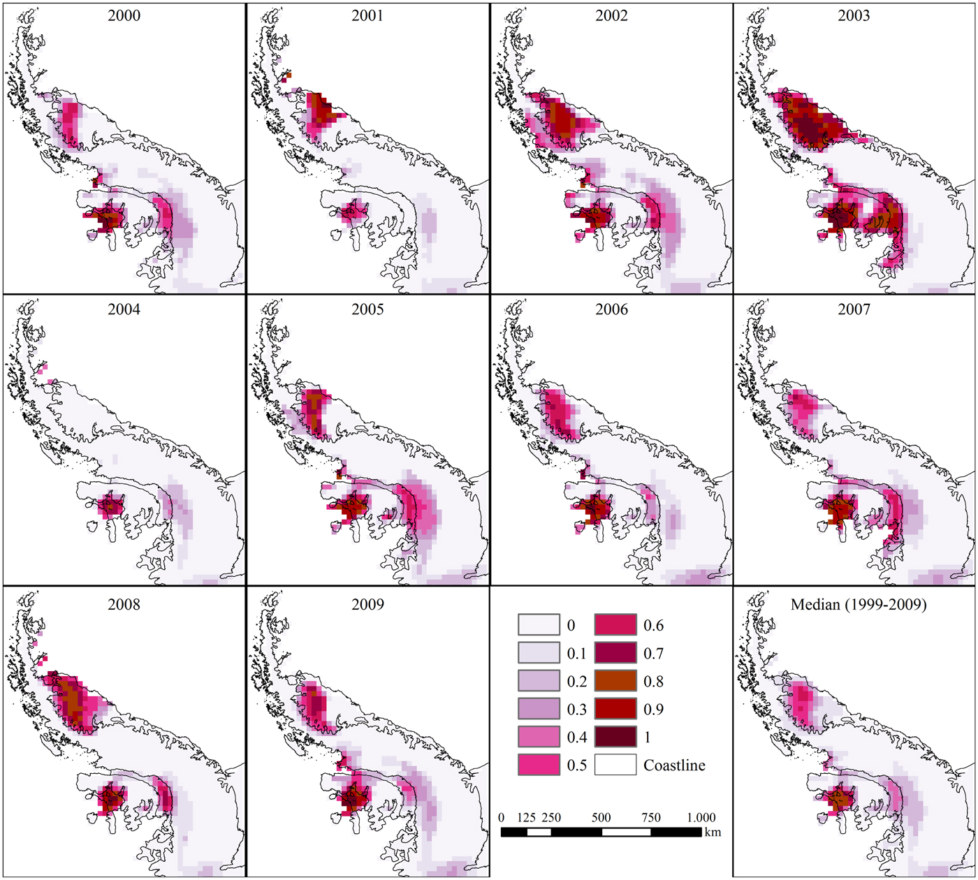
Fig. 3. Annual (1999–2009) median wet-snow fraction in the Antarctic Peninsula during the 3 summer months (December, January, and February) from SSMI time-series images.
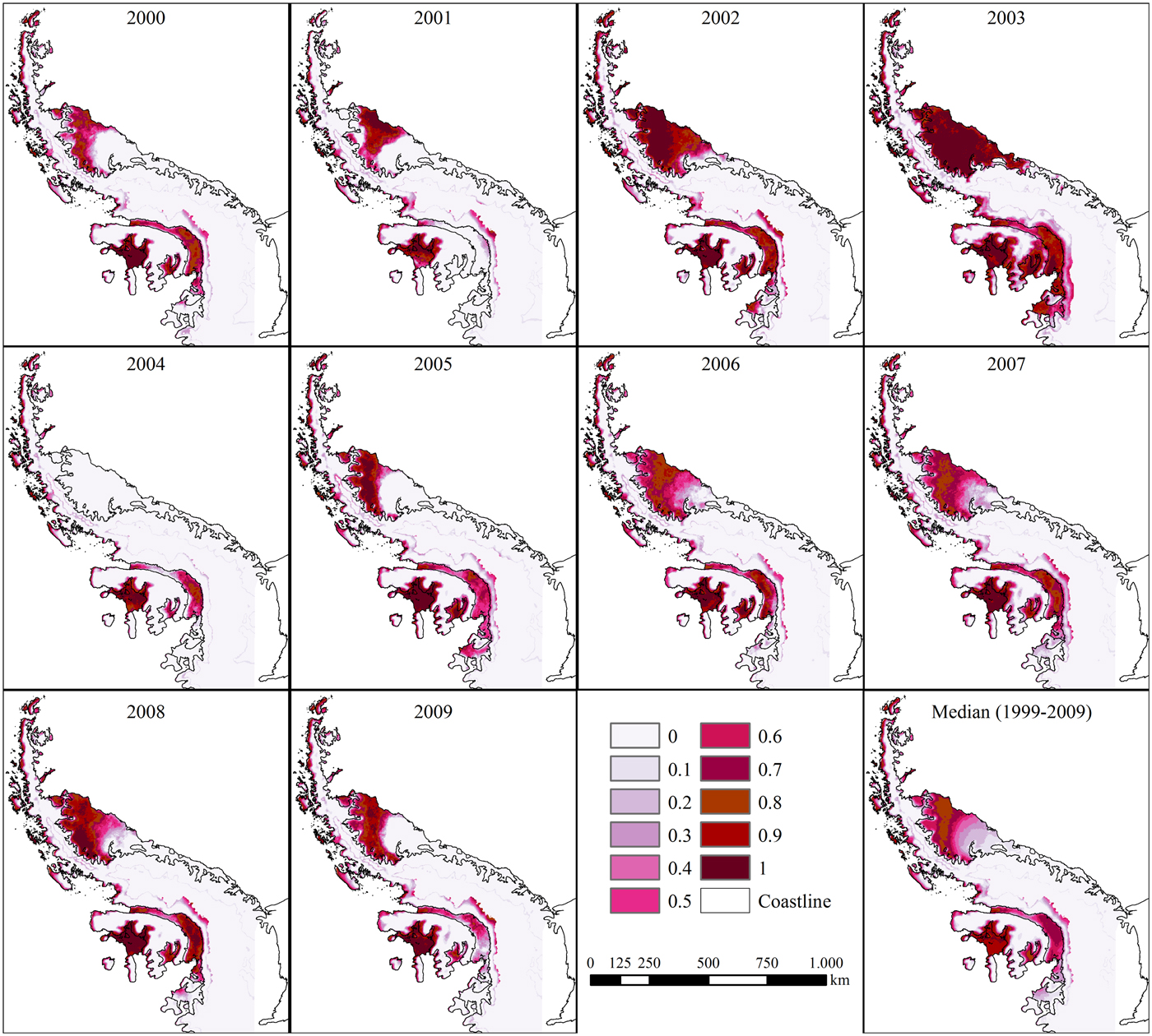
Fig. 4. Annual (1999–2009) median wet-snow fraction in the Antarctic Peninsula during the 3 summer months (December, January, and February) from QuikSCAT time-series images.
Relative to the total extent of the daily wet-snow fraction (sum of all pixel fractions multiplied by the pixel area for each day) measured by the subpixel analysis on SSMI and QuikSCAT, the results show similar spatiotemporal patterns, as shown in Figure 5. The two summer years (2003 and 2004) show a concentration of snow melt during the summer months (especially during the 90 days from December to February, with the highest values in January) beginning in November and finishing approximately by the end of April, especially during the 90 days from December to February, with the highest values in January. The SSMI wet-snow fraction extent was lower than that of QuikSCAT during the winter months and higher in the summer months, as expressed by the expected higher sensitivity for snow-melt detection of data with a higher spatial resolution. Subpixel analysis of the wet-snow fraction-image time series showed results similar to those of another analysis in the Antarctic Peninsula conducted in the same period of the year using Boolean detection approaches (Liu and others, Reference Liu, Wang and Jezek2006; Tedesco, Reference Tedesco2009; Trusel and others, Reference Trusel, Frey and Das2012; Barrand and others, Reference Barrand2013). Spatially, the superficial snow melt in the Antarctic Peninsula was concentrated in the Larsen C, King George VI, and Wilkins ice shelves and is temporally concentrated during the summer months.
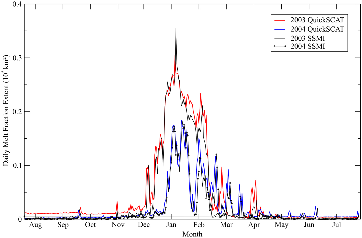
Fig. 5. Daily wet-snow fraction melt extent during the 2003 and 2004 summer years estimated from SSMI and QuikSCAT time-series images.
Evaluation of subpixel mixture analysis based on the wet-snow fraction image timeseries
QuikSCAT multitemporal backscatter band ratio-based masking
The QuikSCAT multitemporal backscatter band ratio of H polarization images allowed masking of persistent-over-time low responses of σ 0 likely related to topographical shadowing effects, probably related to the Peninsula Antarctic Plateau relief (Fig. 6b). The topographical shadowing effects are difficult to be evaluated since the SIRF algorithm developed for generation of QuikSCAT slice-mode images combines σ 0 measurements from multiple azimuth angles and multiple orbit passes collected over the imaging period to generate the enhanced resolution images (Early and Long, Reference Early and Long2001). It is possible that problems related to topographical shadowing effects caused an overestimation of melt metrics and wet-snow fraction images for more than 300 days in each year (Fig. 6a), especially in the Dyer and Bruce Plateaus. The RAMP DEM geomorphometric data (Liu and others, Reference Liu, Jezek, Li and Zhao2001) (Fig. 6b) and the DEM-derived shaded relief image (Fig. 6c) support the hypothesis of topographical shadowing effects on the σ 0 measurements of the QuikSCAT slice mode images. We refer to this overestimation effect as the wet-snow anomaly. The ratio between the QuikSCAT H polarization images from the 2003 winter (Fig. 6d) and summer (Fig. 6e) produced the multitemporal backscatter band ratio mask (Fig. 6f) used to minimize such imaging topography-related problems.
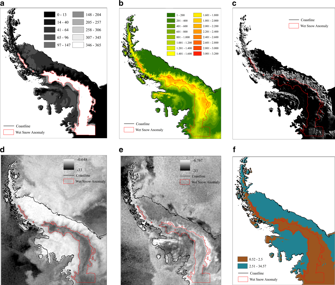
Fig. 6. (a) wet-snow anomaly of the year 2003 (number of days with wet-snow fraction higher than 0.1); (b) RAMP DEM of Antarctic Peninsula (Liu and others, Reference Liu, Jezek, Li and Zhao2001); (c) shaded relief image (sun elevation 45° and azymuth 0°); (d) winter (April 1st, 2003) QuikSCAT H polarization backscatter image; (e) summer (December 31, 2003) QuikSCAT H polarization backscatter image; (f) multitemporal backscatter H polarization band ratio.
SSMI and QuikSCAT wet-snow fraction images assessment
Assessment of SSMI and QuikSCAT wet-snow fraction images based on 11 ASAR classified images shows similar behavior for the subpixel analysis of both datasets, with a slightly better performance by QuikSCAT (as expected due to its higher spatial resolution). As shown in Table 2, the correlation between SSMI and QuikSCAT wet-snow fraction images and the ASAR wet-snow estimated fractions ranged from notably low to high (Pearson's r ranging from 0.01 to 0.86) with the same behavior of the Kappa statistics (ranging from 0 to 0.81), and the RMSE was <0.088 in all images (except for one date with RMSE <0.26). The low correlation for 4 dates is likely due to the use of mosaics of ASAR classified images with different dates.
Table 2. Assessment results of the SSMI and QuikSCAT wet-snow fraction images
*Not significant (p-value > 0.05).
The SSMI wet-snow fraction images (n = 608) had low correlations (r <0.13) for four dates (one in November, two in February, and one in March), medium correlations (r from 0.31 to 0.67) for three dates (one in December and two in February) and high correlations (r from 0.78 to 0.86) for four dates (one in December and three in January). The kappa statistics revealed poor classification κ <0.07) for five dates, regular classification results (κ from 0.32 to 0.66) for five dates and good results (κ = 0.77) for one date. The RMSE was <0.06 in all dates, except for one date with 0.29, pointing to low errors in general.
The QuikSCAT wet-snow fraction images (n = 90 856) presented low correlations (r <0.08) for four dates (one in November, one in December, and two in February), medium correlations (r from 0.44 to 0.57) for three dates (one in December, one in February, and one in March) and high correlations (r from 0.73 to 0.82) for four dates (one in December and three in January). The kappa statistics revealed poor classification (κ <0.02) for four dates, regular classification results (κ from 0.4 to 0.49) for three dates and good classification results (κ from 0.7 to 0.81) for four dates. The RMSE was <0.09 in all dates, except for two dates (0.12 and 0.27, respectively), also revealing low errors in general.
From a regional scale analysis (Fig. 7), the average residual (difference between SSMI and QuikSCAT wet-snow fraction images predicted by subpixel analysis and ASAR classified wet-snow fractions on 11 dates) showed higher results in the Larsen C, King George VI and Wilkins ice shelves. The QuikSCAT residual average (Fig. 7a) ranged from −0.82 to 0.95, with a higher and positive average in King George VI and Wilkins ice shelves, whereas the SSMI residual average (Fig. 7b) ranged from −0.51 to 0.25, with a higher and positive average in King George VI and Wilkins ice shelves and negative average in the Larsen C ice shelf. These snow-melting patterns can be related to the interaction of factors as: (a) ASAR images are more sensitive to slight alterations of the snowpack than SSMI-S and QuikSCAT, which presents an overestimation trend of snow-melting detection; (b) different topographic conditions (lower average slope and rocks presence) of Larsen C compared with King George VI and Wilkins ice shelves (Ku channel is influenced by high slopes).

Fig. 7. Residual average maps of the 11 assessment dates for wet-snow fraction images of QuikSCAT (a) and SSMI (b).
The average residual probability distributions were similar for SSMI and QuikSCAT, mostly in the 0–0.2 interval (QuikSCAT) and in the −0.2 to 0.2 interval, (SSMI) as shown in the kernel probability density plot (Fig. 8). Greater residuals have a notably low probability, and this plot also shows an overestimation trend for the QuikSCAT and SSMI wet-snow fraction estimates. This overestimation was clearer in the QuikSCAT, whereas the SSMI had a more widely distributed residual average trend with a greater presence of underestimated wet-snow fractions.
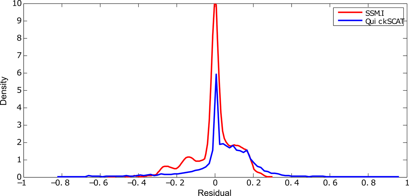
Fig. 8. Kernel probability density plot of the residuals between QuikSCAT and SSMI wet-snow fraction images and ASAR classified images.
SSMI and QuikSCAT melt metrics
The results of the sensitivity analysis on the melt metrics estimated using wet-snow fraction images ranged from 0.1–1 to 0.65–1 for consideration of the presence of snow melt, thus demonstrating a higher amplitude of the melt extent (Table 3) and melt index (Table 4) from the SSMI wet-snow fraction-image time series from a minimum in the summer of 2004 (0.233 106 km2 for melt extent and 3.06 106 km2 days for melt index at the 0.65 lower threshold) to a maximum melt extent in the summer of 2003 (0.54 106 km2 at the 0.1 lower threshold) and the maximum melt index in the summer of 2005 (27.25106 km2 days at the 0.1 lower threshold). The QuikSCAT-based wet-snow fraction-image time series generated a lower amplitude of melt extent (Table 5) and melt index (Table 6) from the minimum in the summer of 2004 (0.24106 km2 and 5.27106 km2 days, respectively, at the 0.65 lower threshold) to the maximum melt extent and melt index in the summer of 2003 (0.375 106 km2 and 26.35106 km2 days, respectively, at the 0.1 lower threshold).
Table 3. Melt extent (106 km2) from SSMI wet-snow fraction images with different ranges with lower limits from 0.1 to 0.65
Table 4. Melt index (106 km2 days) from SSMI wet-snow fraction images with different ranges with lower limits from 0.1 to 0.65

Table 5. Melt extent (106 km2) from QuikSCAT wet-snow fraction images with different ranges with lower limits from 0.1 to 0.65
Table 6. Melt index (106 km2 days) from QuikSCAT wet-snow fraction images with different ranges with lower limits from 0.1 to 0.65

In general, the melt dynamics metrics based on subpixel mixture analysis presented medium to high and significant correlations with the melt metrics estimated by adopting a Boolean approach (Trusel and others, Reference Trusel, Frey and Das2012) with the QuikSCAT egg-mode data (spatial resolution of 4.45 km). According to the different empirically tested ranges, the melt extent from the SSMI subpixel data presented correlation via Pearson's r ranging from 0.69 to 0.83 (n = 10, p ≤ 0.03) and R 2 from 0.47 to 0.69 (Table 3), whereas the QuikSCAT-based melt extent presented a higher correlation with r from 0.85 to 0.88 (n = 10, p ≤ 0.002) and R 2 ranging from 0.73 to 0.77 (Table 5). The melt index based on SSMI subpixel data presented correlation via Pearson's r ranging from 0.72 to 0.91 (n = 10, p ≤ 0.02) and R 2 from 0.52 to 0.83 (Table 4), whereas the QuikSCAT-based melt index also presented a higher average correlation with r from 0.83 to 0.9 (n = 10, p ≤ 0.003) and R 2 from 0.7 to 0.8 (Table 6).
Comparing the SSMI (pixel size = 25 km) and QuikSCAT (pixel size = 2.25 km) wet-snow fraction images based on melt metrics and considering the snow-melt presence, a wet-snow fraction of pixels >0.2, and the melt metrics reference (Trusel and others, Reference Trusel, Frey and Das2012) based on the QuikSCAT egg-mode data (pixel size = 4.45 km), a pattern related to scale (spatial resolution) occurred in the melt extent estimates, which grew by increasing the spatial resolution (Fig. 9). This scale-related pattern highlighted the strong influence of pixel area on the calculation of melt extent with finer resolution data detecting lower melt extent results.
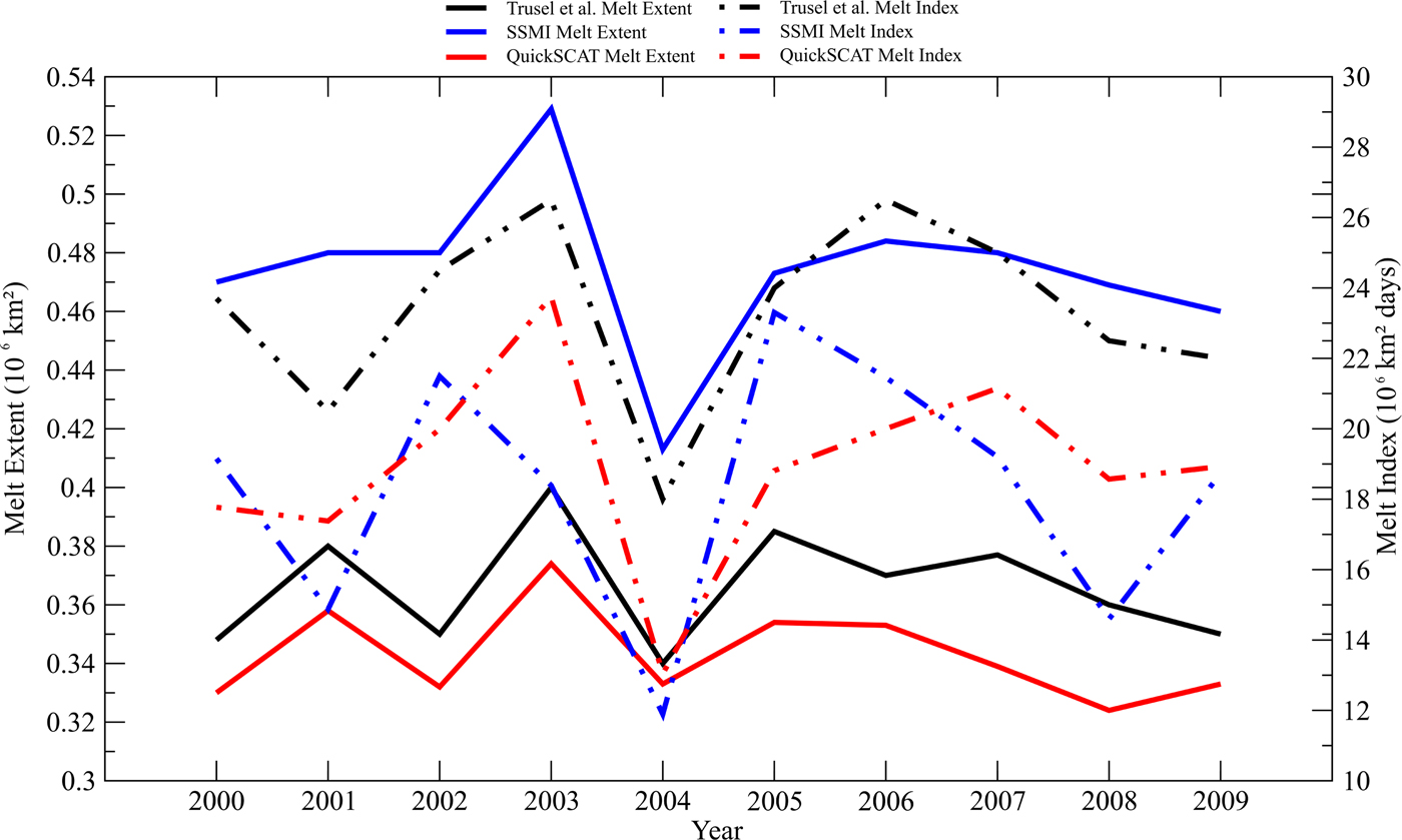
Fig. 9. Melt metrics measured by the reference QuikSCAT (Trusel and others, Reference Trusel, Frey and Das2012) and by the wet-snow fraction images of QuikSCAT and SSMI (using a fraction threshold of 0.15 for snow-melt presence.
The comparison presented by Trusel and others (Reference Trusel, Frey and Das2012) of melt metrics generated by different Boolean approaches with SSMI and QuikSCAT data for the Antarctic continent showed an opposite pattern with higher resolution data producing higher melt extent estimates. Such an opposite pattern could be related to the different snow-melt detection approaches (subpixel vs Boolean analysis) wherein the subpixel analysis presented higher snow-melt sensitivity reflected especially when using lower thresholds (e.g. 0.2) for measurement of melt metrics designed for Boolean detection approaches (considering the presence or absence of snow melt at each pixel). In the case of SSMI melt extent measures, higher wet-snow fraction-image thresholds (>0.55) produced estimates lower than the reference due to the lower number of pixels considered as snow melt at these thresholds.
The melt index estimates, which consider both the extent and the frequency of snow melt, did not follow the same clear scale-related pattern with SSMI and QuikSCAT wet-snow fraction-image-based measures that were quite similar (SSMI melt index slightly higher). In contrast, the reference QuikSCAT melt index (Trusel and others, Reference Trusel, Frey and Das2012) presented higher estimates compared with the SLMM-based estimates with low thresholds (e.g. 0.1). The melt index measures pattern from the SSMI and QuikSCAT wet-snow fraction-image data can be explained by the higher number of snow-melt days in the QuikSCAT interannual time series, and thus, the higher area of the SSMI pixel is minimized by the lower frequency of snow-melt detection. The higher estimates of melt index from the reference (Trusel and others, Reference Trusel, Frey and Das2012) could be related to several possible factors such as measurement method differences (e.g. Boolean and subpixel analysis approaches, use of the multitemporal noise mask) and use of other QuikSCAT image modes (e.g. spatial resolution, incidence angle, noise patterns, and reconstruction algorithm).
CONCLUSIONS
In general, subpixel analysis demonstrated efficient performance for snow-melt detection with both SSMI and QuikSCAT sensors, as shown by evaluation analysis of wet-snow fraction images compared with higher-spatial-resolution ASAR classified images as well as of the derived temporal dynamics melt indices compared with the traditional melt metrics measured by Boolean snow-melt detection approaches in the literature reference (Trusel and others, Reference Trusel, Frey and Das2012; Barrand and others, Reference Barrand2013). Multitemporal band ratio-based maskings were required for QuikSCAT data due to topographical-related effects that produced low backscattering responses. The assessment based on ASAR classified images presented regular to good results according to correlation and error statistics analyses, except for certain days, probably due to the use of multiple passing date image mosaics.
Because the snow melt actually occurs at pixel fractions, the performed multiscale analysis suggests an overestimation of melt metrics calculated according to Boolean approaches that assume all of the areas of the pixels are detected as the presence of snow melt. Because the traditional melt metrics are based on Boolean snow-melt detection, sensitivity analysis is required to evaluate the melt metric results derived from the subpixel analysis. The measured melt metrics show an overestimation as the spatial resolution decreases, an observation related to the multiplicative effect of a larger pixel area. The proposed subpixel analysis is an innovative and consistent approach that offers potential for snow-melt detection and melt metrics measurement.
ACKNOWLEDGMENTS
The authors are grateful for Postdoctoral Fellowship by the PNPD Program (Project No.2764/2010) from the Brazilian Federal Agency for Support and Evaluation of Graduate Education within the Ministry of Education of Brazil (CAPES) and for financial support from the Brazilian National Council for Scientific and Technological Development (CNPq) and the Project Brazilian National Institute for Cryospheric Sciences (Process No. 465680/2014-3). J. Arigony-Neto and J.C. Simes acknowledge CNPq research grants.


 Open access