


1. Introduction
Trapped modes (TMs) in acoustics and water waves are those special natural modes of free oscillation in open continuous systems that do not radiate energy to infinity. In contrast, natural modes that radiate energy are leaky modes (LMs). The temporal properties or definitions of TMs and LMs are respectively the modal oscillations non-decaying and decaying in time, i.e. the harmonic modal oscillations with real and complex frequencies. Trapped modes residing inside a continuous frequency range of propagating waves that can radiate energy to infinity are called embedded TMs, or bound states in the continuum (BICs). The concept of TMs was introduced by Ursell (Reference Ursell1951) and the possibility of BICs was proposed earlier by von Neumann & Wigner (Reference von Neumann and Wigner1929a). Comprehensive reviews of the literature can be found in Linton & McIver (Reference Linton and McIver2007) and Hsu et al. (Reference Hsu, Zhen, Stone, Joannopoulos and Soljac̆ić2016). Studies have demonstrated significant influences of TMs and slightly LMs on vortex structures (Peters Reference Peters1993; Tonon et al. Reference Tonon, Golliard, Hirschberg and Ziada2011), on flow instabilities (Yamouni, Sipp & Jacquin Reference Yamouni, Sipp and Jacquin2013; Towne et al. Reference Towne, Cavalieri, Jordan, Colonius, Schmidt, Jaunet and Brés2017; Martini, Cavalieri & Jordan Reference Martini, Cavalieri and Jordan2019; Dai Reference Dai2021b) and on wave scattering (Bennetts, Peter & Craster Reference Bennetts, Peter and Craster2018; Bobinski et al. Reference Bobinski, Maurel, Petitjeans and Pagneux2018; Zheng, Porter & Greaves Reference Zheng, Porter and Greaves2020). This study, however, still focuses on the TM phenomenon itself (Callan, Linton & Evans Reference Callan, Linton and Evans1991; Duan et al. Reference Duan, Koch, Linton and McIver2007; Hein, Koch & Nannen Reference Hein, Koch and Nannen2012; Newman Reference Newman2018).
A natural mode of a dynamical system represents a pattern of small oscillation without an excitation source in which all parts of the system oscillate harmonically with the same frequency. Mathematically, natural modes of a continuous system are solutions of a differential eigenvalue problem determining the values of the constant  $\omega$ (eigenvalues) so that the differential equation with respect to space admits non-trivial solutions (eigenfunctions) satisfying boundary conditions (Courant & Hilbert Reference Courant and Hilbert1989). The eigenvalues are modal frequencies and the eigenfunctions are modal shapes. In some cases, such as for the eigenmodes of transverse vibration in a uniform string with two fixed ends and of acoustic oscillation in a closed rectangular cavity, the differential eigenvalue problem can be solved analytically. In many cases, such as for eigenmodes in a non-uniform string and in an open acoustic resonator, the problem is usually transformed into an algebraic eigenvalue problem and then solved numerically. The eigenvalues and eigenvectors solved from the algebraic eigenvalue problem are or lead to the approximations of the eigenvalues and eigenfunctions of the original differential eigenvalue problem. The transformation can be achieved by means of such as spatial discretization and modal expansion (Meirovitch Reference Meirovitch1997). The modal expansion method, that is, expanding the eigenfunctions of the system yet to be solved in terms of the known eigenfunctions of a self-adjoint system, relies on the orthogonality and completeness of an infinite set of modes of the self-adjoint system. It is also referred to as coupled-mode theory (Haus Reference Haus1984; Joannopoulos et al. Reference Joannopoulos, Johnson, Winn and Meade2008). Spatial discretization and modal expansion methods have been developed to calculate eigenmodes of open acoustic resonators (Hein, Hohage & Koch Reference Hein, Hohage and Koch2004; Lyapina et al. Reference Lyapina, Maksimov, Pilipchuk and Sadreev2015), and the numerical eigenvalues being real or complex indicates the solved eigenmodes being TMs or LMs. However, as mentioned in Linton & McIver (Reference Linton and McIver2007), it is not a rigorous way of distinguishing truly TMs from slightly LMs, owing to numerical discretization or modal truncation.
The existence proofs of TMs are usually obtained via the variational formulation of the differential eigenvalue problem based on Rayleigh's quotient (Meirovitch Reference Meirovitch1997). For embedded TMs, the general proof strategy relies on an operator decomposition (Linton & McIver Reference Linton and McIver2007). One first finds an operator whose continuous spectrum of propagating waves that can radiate energy to infinity is bounded away from the origin  $[\omega _c, \infty )$ by a suitable operator decomposition, then proves the existence of eigenvalues in the gap
  $( 0, \omega _c )$ via a variational principle. The following three types of embedded TMs have been successfully proved by this strategy. Moreover, because some geometrical properties of the systems are needed in the operator decomposition, this strategy also reveals the connection between the mechanisms of those TMs and the particular geometrical properties of the systems. The first type is referred to as symmetry-protected TMs. For example,
  $y$-antisymmetric TMs occur in a two-dimensional (2-D) Neumann waveguide containing obstacles or cavities symmetric about the guide centreline, explained by the symmetry mismatch between TMs and the radiating waves in the guide. This type of TM was first encountered in flow ducts containing plates (Parker Reference Parker1966). With an operator decomposition, Evans, Levitin & Vassiliev (Reference Evans, Levitin and Vassiliev1994) proved the existence of at least one TM in a Neumann waveguide with any symmetric obstacle placed on the guide centreline. The second type is referred to as invisibility-protected TMs, appearing in a waveguide containing one or multiple zero-thickness plates, thus they are only of theoretical interest. If the normal of the plates is perpendicular to the generators of the guide, TMs can occur owing to that some guided waves in the guide are not scattered by the plates (or one may say that the plates are invisible to those waves) (Evans, Linton & Ursell Reference Evans, Linton and Ursell1993; Davies & Parnovski Reference Davies and Parnovski1998; Groves Reference Groves1998; Linton & McIver Reference Linton and McIver1998; Linton et al. Reference Linton, McIver, McIver, Ratcliffe and Zhang2002). The third type, referred to as symmetry–periodicity-protected TMs, was found by Utsunomiya & Eatock Taylor (Reference Utsunomiya and Eatock Taylor1999) and Porter & Evans (Reference Porter and Evans1999) in a 2-D waveguide containing
  $N \geq 2$ identical obstacles at the same
  $x$-position that form an
  $N$-period section of an infinite array of equally spaced obstacles in the
  $y$-direction. With
  $N$ periods,
  $N$ patterns of TMs can be found in a 2-D Neumann waveguide. Linton & McIver (Reference Linton and McIver2002) proved the existence of those TMs and revealed that symmetry-protected TMs are a special case of symmetry–periodicity-protected TMs with
  $N=1$. Note the relation between TMs and Rayleigh–Bloch waves in periodic structures (Porter & Evans Reference Porter and Evans1999; Linton & McIver Reference Linton and McIver2002): travelling Rayleigh–Bloch waves in the opposite directions comprise standing TMs.
However, a fourth type of embedded TM, referred to as Friedrich–Wintgen TMs by some authors, cannot yet be proved and explained by the operator decomposition approach, because ‘a decomposition which places them below the essential spectrum of some operator does not exist (or has not been found)’ (Linton & McIver Reference Linton and McIver2007). The most notable difference between the fourth type and the first three types above is that TMs of the fourth type occur discretely whereas TMs of the first three types occur continuously in a two-parameter space. The reader is referred to figure 2 in Duan et al. (Reference Duan, Koch, Linton and McIver2007) and figure 5 in Hein et al. (Reference Hein, Koch and Nannen2012) for a clear comparison of the two different features. Linton & McIver (Reference Linton and McIver2007) described the two different features by unstable and stable TMs and Hsu et al. (Reference Hsu, Zhen, Stone, Joannopoulos and Soljac̆ić2016) classified the fourth type as bound states through parameter tuning. In this paper, the fourth type of TMs are categorized as accidental TMs, considering an analogy between those TMs and accidental degeneracy (McIntosh Reference McIntosh1959; Greenberg Reference Greenberg1966), whereas the first three types are just categorized as common TMs.
There are two kinds of previous understandings on the mechanism of accidental TMs, which are totally different from those drawn from the operator decomposition approach for common TMs. Using the Feshbach projection operator formalism, Friedrich & Wintgen (Reference Friedrich and Wintgen1985) related the existence of BICs to the avoided crossing between the loci of two eigenvalues as a continuous parameter of the system is varied. An accompanying phenomenon of the avoided crossing is the bifurcation of resonance widths into long-lived and short-lived resonances, i.e. one eigenvalue has a local minimum in the imaginary part whereas the other has a local maximum. The synchronicity between accidental TM, avoided crossing and resonance-width bifurcation as a system parameter is varied has been reported in almost all researches on accidental TMs, as reviewed by Okołowicz, Płoszajczak & Rotter (Reference Okołowicz, Płoszajczak and Rotter2003), Rotter (Reference Rotter2009), Hsu et al. (Reference Hsu, Zhen, Stone, Joannopoulos and Soljac̆ić2016) and Sadreev (Reference Sadreev2021). Considering the synchronicity and especially the fact that accidental TMs reside at locations of local minima of the imaginary part of eigenvalues, it is natural to conjecture that accidental TMs are a result of avoided crossing and resonance-width bifurcation. Since the work of Friedrich and Wintgen in 1985, the two behaviours of eigenvalue loci near TMs have often been understood as the mechanism of those TMs and have always been used as predictive indicators for the occurrence of accidental TMs. The second kind of understanding, less popular, is to relate the mechanism of accidental TM in an open cavity–waveguide system to the phenomenon of modal degeneracy in a corresponding closed cavity (Lyapina et al. Reference Lyapina, Maksimov, Pilipchuk and Sadreev2015; Sadreev Reference Sadreev2021).
The objective of this paper is to reveal the commonality and difference between the mechanisms of common and accidental TMs based on a unified theoretical analysis. To accomplish the unified analysis, the first idea is that all TMs can be explained by only examining the eigenfunctions of the TMs themselves, disregarding the loci of eigenvalues. This idea is in contrast to the popular approach for accidental TMs, i.e. varying the system and tracing eigenvalue loci. Second, we define TMs by means of two conditions, i.e. the eigenmode condition and the wave-trapping (zero-radiation) condition, formulate them with the travelling-wave components of the eigenfunctions and then analyse why and how the travelling-wave components of the eigenfunctions can satisfy the eigenmode and wave-trapping conditions simultaneously. The idea of mutual cancellation in radiation into the waveguide between waves or submodes in the resonant region of an eigenfunction can be found in such as Linton & McIver (Reference Linton and McIver2007) and Hsu et al. (Reference Hsu, Zhen, Stone, Joannopoulos and Soljac̆ić2016). However, the zero-radiation condition has not been combined with the eigenmode condition in previous eigenfunction analyses. Third, we limit the present investigation to segmented-homogeneous resonator–waveguide systems, so that the eigenfunctions can be rigorously decomposed into duct modes (DMs) in each homogeneous segment of the systems, which ultimately transforms the analysis of TMs to the analysis of DM propagation and scattering.
The paper is organized as follows. Section 2 presents the basic definition of TMs, i.e. the eigenmode and wave-trapping conditions, the travelling-wave formulations of the two conditions and the computational model. Section 3 describes the eigenfunctions and their travelling-wave components of different types of TMs. Section 4 investigates and compares the mechanisms of various types of TMs by analysing in each case why and how the travelling-wave components of the eigenfunctions can satisfy the TM conditions simultaneously. In contrast to previous studies, § 5 discusses that phenomena such as modal degeneracy, avoided crossing and resonance-width bifurcation are not the mechanisms of accidental TMs. Section 6 concludes the paper.
2. Definition, fundamental principle and computational model
2.1. The first condition of TMs: eigenmode condition
Lifshitz & Pitaevskii (Reference Lifshitz and Pitaevskii1981) derived a general travelling-wave formulation of the eigenmode condition of continuous systems. For the present problem sketched in figure 1, i.e. eigenmodes in a 2-D acoustic waveguide containing cavities or plates in the resonant region from  $x=0$ to
  $x=L$, the travelling-wave interpretation is that an eigenmode may be regarded as resulting from the superposition of travelling waves in the
  $\pm x$ directions reflected by the region boundaries at
  $x=0$ and
  $x=L$. Since the eigenfunction is one valued, such a travelling-wave decomposition leads to the characteristic condition of the eigenmode, that is, the travelling waves remain unchanged after a loop or round trip of propagation and reflection in the resonant region. For cases with a sufficiently long resonant region, i.e.
  $L \gg 1$, the influences of
  $k^{\mp }_e$ cut-off DMs (evanescent waves) generated by the scattering of
  $k^{\pm }_p$ cut-on DMs (propagating waves) at one end on the wave scattering at the opposite end and on the loop characteristics can be neglected. The one-valued or the loop closure principle for each eigenmode is then formulated in the asymptotic form (Lifshitz & Pitaevskii Reference Lifshitz and Pitaevskii1981)
 \begin{equation} R_0(\omega)R_L(\omega) \mathrm{exp} \big\lbrace -\mathrm{i} \big[ k^+_p (\omega)- k^-_p (\omega) \big] L\big\rbrace=1, \end{equation}
where  $R_0$ and
  $R_L$ are the reflection coefficients at region boundaries,
  $k^{\pm }_p$ are wavenumbers and the frequency
  $\omega$ can be either real or complex. Note that, for the simplicity of (2.1), it is assumed that only a single propagating wave in the
  $\pm x$ directions is involved in the eigenmode. The loop closure principle includes both magnitude and phase constraints
 $$\begin{gather} |R_0R_L| \mathrm{exp} \big\lbrace \big[ \mathrm{Im} (k^+_p) - \mathrm{Im} (k^-_p) \big] L\big\rbrace = 1, \end{gather}$$
 $$\begin{gather}\mathrm{arg} \left( R_0R_L \right) + \big[ - \mathrm{Re} (k^+_p) + \mathrm{Re} (k^-_p) \big] L =-2m{\rm \pi}, \end{gather}$$
where  $m$ is an integer.

Figure 1. Travelling-wave components of an eigenfunction in an acoustic resonator–waveguide system:  $k^{\pm }_p$ cut-on DMs (propagating waves) in the resonant region,
  $k^{\pm }_r$ cut-on DMs in the waveguide that can radiate energy to infinity if not decoupled and
  $k^{\pm }_e$ cut-off DMs (evanescent waves).
The travelling-wave formulation provides physical insights into the eigenmodes of continuous systems. It reveals that waves travelling in opposite directions and wave reflections at the two ends of the resonant region are four indispensable ingredients of an eigenmode, because the loop must be closed. For acoustics, it also reveals the connection between the system eigenmodes being real or complex and the wave reflection characteristics, illustrated as follows. Assume the resonant region in figure 1 is a 2-D hard-walled duct segment of length  $L$ and height
  $H=1$. Acoustic DMs (Rienstra & Hirschberg Reference Rienstra and Hirschberg2021) in the
  $\pm x$ directions are in the form of
 \begin{equation} p = P(y)\exp(-\mathrm{i} k x)\exp(\mathrm{i} \omega t ), \end{equation}
where  $p$ is the pressure disturbance,
  $P(y)$ is the modal profile. The dispersion relation of DMs is
 \begin{equation} k_n^{{\pm}} ={\pm} \sqrt{\omega^2-\left[ (n-1){\rm \pi} \right] ^2}, \end{equation}
where  $n=1,2,3\ldots$ and
  $n=1$ for the plane waves,
  $k_n^{\pm }$ is the wavenumber of the
  $n$th DM in the
  $\pm x$ directions. All variables are normalized by the sound speed, fluid density and the duct height. As the frequency varies from
  $\omega /{\rm \pi} =1.5-6\mathrm {i}$ to
  $1.5+6\mathrm {i}$, (2.5) is plotted in figure 2 for the first eight DMs in the
  $\pm x$ directions, of which the first two DMs are cut-on (propagating) and the others are cut-off (evanescent). First, consider in figure 1 the duct segment being closed at
  $x=0$ and
  $x=L$ by straight walls, so that
  $R_0=R_L=1$ for each DM. Each pair of
  $k_n^+$ and
  $k_n^-$ cut-on DMs can satisfy (2.2) and form an eigenmode at a real-valued frequency selected by (2.3). Second, consider an open system as in figure 1, so
  $|R_0| \leq 1$ and
  $|R_L| \leq 1$. A pair of
  $k_n^+$ and
  $k_n^-$ cut-on DMs can also satisfy (2.2) and underpin an eigenmode at a real frequency selected by (2.3) if
  $|R_0|=|R_L|=1$ for that pair of DMs. If
  $|R_0R_L|<1$ for a pair of
  $k_n^+$ and
  $k_n^-$ cut-on DMs, then a real-frequency eigenmode cannot be formed by that pair. Nevertheless, a positive
  $\mathrm {Im}(\omega )$ leads to
  $\mathrm {exp} \lbrace [\mathrm {Im} (k_n^+) - \mathrm {Im} (k_n^-) ] L\rbrace >1$ for cut-on DMs (see figure 2), thus (2.2) can be satisfied at a complex frequency selected by (2.2) and (2.3). So, it is total reflection or not rather than an acoustic system being geometrically closed or open that decides eigenmodes of the system being real or complex. A pair of
  $k_n^+$ and
  $k_n^-$ cut-off DMs always leads to
  $\mathrm {exp} \lbrace [ \mathrm {Im} (k_n^+) - \mathrm {Im} (k_n^-) ] L\rbrace <1$ at either real or complex frequencies (see figure 2), thus, without the participation of propagating waves, pairs of
  $k_n^+$ and
  $k_n^-$ evanescent waves alone cannot satisfy (2.2) and therefore cannot form an eigenmode.

Figure 2. Dispersion relation in a 2-D hard-walled acoustic waveguide of height  $H=1$. (a) Complex frequency and (b) wavenumbers of the first eight
  $\pm x$ DMs.
2.2. The second condition of TMs: wave-trapping condition
There are spatial and temporal approaches of defining some special eigenmodes in an open system as TMs. In the spatial approach, the most commonly used definition is zero radiation. Specifically, the eigenfunction of a TM has no travelling-wave components that can radiate to infinity. In resonator–waveguide systems, this occurs in two different situations. One is that the system eigenmodes occur in a frequency range where all DMs in the infinite waveguide are cut-off, which can happen in waveguides with the Dirichlet boundary condition (Pagneux Reference Pagneux2013). The other situation is that there are cut-on DMs in the waveguide, but they do not participate in (or they are decoupled from) some eigenmodes of the system. In other words, the amplitudes or mode coefficients of  $k^{\pm }_r$ cut-on DMs in figure 1 are zero if the eigenfunctions are decomposed into DMs
 \begin{equation} C^{{\pm}}_r=0. \end{equation}
In contrast, system eigenmodes with  $C^{\pm }_r \neq 0$ are LMs. Trapped modes in the second situation are called embedded TMs or BICs (Hsu et al. Reference Hsu, Zhen, Stone, Joannopoulos and Soljac̆ić2016), since there are cut-on DMs in the waveguide when the TMs occur. All acoustic TMs in this study are embedded TMs, because the Neumann boundary condition leads to the cut-on plane wave in the waveguide at all frequencies.
In the situation of  $L \gg 1$, if one neglects the influences of
  $k^{\mp }_e$ cut-off DMs generated by the scattering of
  $k^{\pm }_p$ cut-on DMs at one end on the wave scattering at the opposite end, the following two equivalents to the zero-radiation condition (2.6) can be easily obtained: the zero transmission from
  $k^{\pm }_p$ cut-on DMs inside the resonant region respectively to the outgoing
  $k^{\pm }_r$ cut-on DMs in the infinite waveguide
 \begin{equation} T_L = T_ 0 =0, \end{equation}
and the total reflection of  $k^{\pm }_p$ cut-on DMs at the region boundaries
 \begin{equation} \left| R_L \right|=\left| R_0 \right|=1. \end{equation}
The temporal approach of defining TMs is that the free oscillation associated with an eigenmode of an open system does not decay in time, i.e. the modal frequency is real
 \begin{equation} \mathrm{Im}(\omega_{TM})=0. \end{equation}
In contrast,  $\mathrm {Im}(\omega _{LM})>0$ under the
  $\exp (\mathrm {i} \omega t )$ convention.
One can obtain the equivalence between (2.6) and (2.9) from an obvious physical statement in this context (no other gains and losses) that spatially zero energy radiation is equal to temporally neutral free oscillations. Here, the equivalence of these four conditions that define some special eigenmodes of an open system as TMs is discussed based on the sketch of figure 1, where we assume a single cut-on DM in the  $\pm x$ directions. In cases where multiple cut-on DMs are involved, the equivalence between zero radiation, zero transmission, total reflection and real modal frequency still holds in the physical sense, although (2.6), (2.7) and (2.8) need to be accordingly generalized (see § 4).
2.3. Computational model
The present resonator–waveguide systems are divided into homogeneous duct segments. The DMs are given by
 \begin{equation} k_n^{{\pm}} ={\pm} \sqrt{ \omega^2-\left[ (n-1){\rm \pi} /H_j\right] ^2}, \end{equation}
for wavenumbers and
 \begin{equation} P_n(y) = \mathrm{cos} \left[ (n-1){\rm \pi} y/H_j \right]\!, \end{equation}
for modal profiles, where  $H_j$ is duct height and
  $j$ is the index of ducts. The DMs are normalized so that
  $|P_n(y) |_{max}=1$. The eigenfunction of a system eigenmode is expanded in terms of DMs in each duct with coefficients
  $C_{n,j}^{\pm }$ to be determined
 \begin{equation} p_j(x,y) = \sum_{n=1}^{N_j} C_{n,j}^{{\pm}} P_{n,j}(y) \exp(-\mathrm{i} k_{n,j}^{{\pm}} x), \end{equation}
where DMs in the  $\pm x$ directions in the resonant region and outgoing DMs in the two semi-infinite waveguides are involved in the summation.
A loop matrix taking into account cut-on and cut-off DMs in the resonant region is defined (Doaré Reference Doaré2001; Gallaire & Chomaz Reference Gallaire and Chomaz2004; Doaré & de Langre Reference Doaré and de Langre2006; de Lasson et al. Reference de Lasson, Kristensen, Mørk and Gregersen2014; Dai Reference Dai2021a)
 \begin{equation} \boldsymbol{\mathsf{M}}_{lp} = \boldsymbol{\mathsf{R}}_{l}\boldsymbol{\mathsf{P}}_{l}\boldsymbol{\mathsf{R}}_r\boldsymbol{\mathsf{P}}_{r}. \end{equation}
In the calculations,  $N$ less attenuated DMs in the
  $\pm x$ directions in the
  $H=1$ infinite waveguide are used and the number of less attenuated DMs used in duct segment(s) in the resonant region is accordingly
  $N_j=NH_j/H$. So, the total number of DMs in the
  $\pm x$ directions in the resonant region is
  $N_t=\sum N_j$. Here,
  $\boldsymbol{\mathsf{P}}_l (N_t \times N_t)$ and
  $\boldsymbol{\mathsf{P}}_r (N_t \times N_t)$ are propagation matrices of the left-running and right-running DMs, describing a wave travelling inside the resonant region;
  $\boldsymbol{\mathsf{P}}_{l,r}$ are diagonal matrices with the elements on the diagonal being
  $\exp ( \pm \mathrm {i} k_n^{\mp } L )$;
  $\boldsymbol{\mathsf{R}}_l (N_t \times N_t)$ and
  $\boldsymbol{\mathsf{R}}_r (N_t \times N_t)$ are the left and right reflection matrices, describing wave reflection at region boundaries;
  $\boldsymbol{\mathsf{R}}_{l,r}$ are extracted from the interface scattering matrices. Using the interface between the resonant region and the right semi-infinite waveguide as an example, the scattering matrix is obtained by numerically matching DMs on both sides of the interface (Kooijman et al. Reference Kooijman, Testud, Aurégan and Hirschberg2008; Kooijman, Hirschberg & Aurégan Reference Kooijman, Hirschberg and Aurégan2010; Dai & Aurégan Reference Dai and Aurégan2018). The continuity of
  $p$ and
  $\partial p/ \partial x$ at the interface and
  $\partial p/ \partial x=0$ on the vertical wall lead to the scattering matrix that links incoming waves to outgoing waves from the interface
 \begin{equation} \left(\begin{array}{@{}c@{}} \boldsymbol{C}_r^+ \\ \boldsymbol{C}_l^- \end{array}\right)= \boldsymbol{\mathsf{S}}\left(\begin{array}{@{}c@{}} \boldsymbol{C}_l^+ \\ \boldsymbol{C}_r^- \end{array}\right)\!, \end{equation}
where vectors  $\boldsymbol {C}^{\pm }_l$ (respectively
  $\boldsymbol {C}^{\pm }_r$) contain coefficients of DMs in the
  $\pm x$ directions on the left and right sides of the interface
 \begin{equation}
\boldsymbol{\mathsf{S}}= \Big(\begin{array}{@{}cc@{}}
\boldsymbol{\mathsf{T}}^+ &
\boldsymbol{\mathsf{R}}^- \\
\boldsymbol{\mathsf{R}}^+ &
\boldsymbol{\mathsf{T}}^- \end{array}\Big)\!,
\end{equation}
\begin{equation}
\boldsymbol{\mathsf{S}}= \Big(\begin{array}{@{}cc@{}}
\boldsymbol{\mathsf{T}}^+ &
\boldsymbol{\mathsf{R}}^- \\
\boldsymbol{\mathsf{R}}^+ &
\boldsymbol{\mathsf{T}}^- \end{array}\Big)\!,
\end{equation}
where  $\boldsymbol{\mathsf{T}}^{\pm }$ and
  $\boldsymbol{\mathsf{R}}^{\pm }$ are transmission and reflection matrices in the
  $\pm x$ directions and
  $\boldsymbol{\mathsf{R}}^+=\boldsymbol{\mathsf{R}}_r$.
The loop closure principle (2.1) requires that an eigenvalue of  $\boldsymbol{\mathsf{M}}_{lp}$ is unity
 \begin{equation} \boldsymbol{\mathsf{M}}_{lp} \boldsymbol{C}_{lp}= k_{lp} \boldsymbol{C}_{lp} \quad \mbox{and}\quad k_{lp} =1. \end{equation}
Since (2.16a,b) is the condition of all eigenmodes, including both TMs and LMs, the temporal definition (2.9) is used in the calculations to distinguish TMs from LMs. For common TMs, the real-valued frequency  $\omega$ is optimized with a given TM length
  $L$, for that an eigenvalue of
  $\boldsymbol{\mathsf{M}}_{lp}$ equals unity. For accidental TMs, both
  $L$ and real-valued
  $\omega$ are optimized. One optimization process solves one TM: the optimized
  $\omega$ is the eigenfrequency and the eigenvector
  $\boldsymbol {C}_{lp}$ corresponding to
  $k_{lp} =1$ contains mode coefficients of DMs, the linear superposition of which gives the eigenfunction. The eigenfunction is normalized so that
  $|p(x,y)|_{max}=1$. In the calculations, the iteration stops when the error between the target
  $k_{lp}$ and unity is less than
  $10^{-12}$, the number of
  $k_n^{\pm }$ DMs in the waveguide with
  $H=1$ varies from
  $N=400$ to 600 (for a round number of
  $N_j=NH_j/H$) and the relative errors of
  $\omega$ and
  $L$ are of the order of
  $10^{-5}$–
 $10^{-6}$ as
  $N$ is doubled in the checked cases: figures 4, 8 and 10.
3. Travelling-wave description of the eigenfunctions of TMs
3.1. Symmetry-protected TMs
The first example of symmetry-protected TMs is in a waveguide with a  $y$-symmetric cavity, as displayed in figure 3. First, the mode coefficients of DMs in figure 3(d,h) indicate the split between
  $y$-antisymmetric and
  $y$-symmetric DMs in the
  $y$-symmetric system. The
  $y$-antisymmetric TMs are composed of only
  $y$-antisymmetric DMs. The only one outgoing cut-on DM (
 $k_1^+$) in
  $d2$ has a zero mode coefficient, indicating zero radiation. Second, only one pair of cut-on DMs (
 $k_2^{\pm }$) in the resonant region (
 $d1$) is involved, as shown in figure 3(b,f). The wave reflection at region boundaries is total reflection, i.e.
  $| R_0 |=| R_L |=1$. Third, the zero mode coefficient of
  $k_1^+$ DM in
  $d2$ also indicates that the transmission from
  $k_2^{\pm }$ DMs in the resonant region to the outgoing
  $k_1^{\pm }$ DMs in the waveguide is zero, i.e.
  $T_0 = T_ L =0$. So, all the three spatial features of TMs, i.e. (2.6), (2.7) and (2.8), are observed.

Figure 3. Trapped modes in a waveguide with a  $y$-symmetric cavity of depth
  $D=2$: (a,e)
  ${\rm Re}(\,p)$ of short and long TMs (
 $L=0.3$,
  $\omega /{\rm \pi} =0.6667$;
  $L=10$,
  $\omega /{\rm \pi} =0.5045$); (b,f)
  ${\rm Re}(\,p)$ of
  $k_2^{\pm }$ cut-on DMs; (c,g)
  ${\rm Re}(\,p)$ of
  $k_4^{\pm }$ cut-off DMs; (d,h) modulus of mode coefficients of
  $k_n^+$ DMs in
  $d1$ and
  $d2$ in the TM eigenfunctions.
Note that, for all TMs in this paper, the number of cut-on DMs in each duct segment is known from the TM frequencies given in figure captions. The cut-on frequency of  $k_n^{\pm }$ DMs is
  $\omega _{{cut\text -on}}/{\rm \pi} = (n-1)/H_j$.
Let us compare the short and long TMs in figure 3. In the short TM,  $k_4^{\pm }$ evanescent DMs in
  $d1$ generated at
  $x=0$ or
  $x=L$ have a non-negligible amplitude at the opposite end, as shown in figure 3(c). On the other hand,
  $k_4^{\pm }$ DMs in the long TM have a quite small amplitude, as shown in figure 3(g). Especially, after a long-distance exponential decrease
  $\exp ( \mp \mathrm {i} k_4^{\pm } L) = 5.33 \times 10^{-20}$,
  $k_4^{\pm }$ DMs have a vanishingly small amplitude at the destinations. So, the long TM is visually clean and simple. It is essentially one pair of
  $k_2^{\pm }$ cut-on DMs in the resonant region with total reflection at region boundaries. The second difference between the short and long TMs is that
  $k_2^{\pm }$ DMs in
  $d1$ show different phase changes in total reflection: figure 3(b) is close to a hard-wall reflection (the phase change is zero and
  $\partial p/ \partial x =0$ at the reflection interface) whereas figure 3(f) is close to a pressure-release reflection (the phase change is
  ${\rm \pi}$ and
  $p=0$ at the reflection interface).
The second example of symmetry-protected TMs is in a waveguide containing a plate placed on the centreline, as displayed in figure 4. The mode coefficients of DMs in  $d3$ indicate the split between
  $y$-antisymmetric and
  $y$-symmetric DMs. The amplitudes of all
  $y$-symmetric DMs in
  $d3$, including the only one cut-on DM (
 $k_1^+$), are zero. The magnitudes of
  $k_n^+$ DMs in respectively
  $d1$ and
  $d2$ are the same, as shown in figure 4(d,h), whereas the phases of
  $k_n^+$ DMs in
  $d1$ and
  $d2$ are the same for
  $y$-antisymmetric DMs but opposite for
  $y$-symmetric DMs (this phase information is not shown in mode coefficients, but it can be seen in figure 4b,c,f,g), which ensures the
  $y$-antisymmetric eigenfunction in the resonant region. In both
  $d1$ and
  $d2$, there is only one pair of cut-on DMs (
 $k_1^{\pm }$), and they have total reflection at the ends, as shown in figure 4(b,f). Visually, the short TM is complicated by evanescent waves, but the long TM is clean and simple, essentially two standing waves oscillating in
  $d1$ and
  $d2$ with equal amplitude and opposite phases. These two standing waves are spatially separated by the plate, however, they are coupled.

Figure 4. Trapped modes in a waveguide with a plate of thickness  $T=0.1$ on the centreline: (a,e)
  ${\rm Re}(\,p)$ of short and long TMs (
 $L=0.3$,
  $\omega /{\rm \pi} =0.9574$;
  $L=10$,
  $\omega /{\rm \pi} =0.0950$); (b,f)
  ${\rm Re}(\,p)$ of
  $k_1^{\pm }$ cut-on DMs; (c,g)
  ${\rm Re}(\,p)$ of
  $k_2^{\pm }$ cut-off DMs; (d,h) modulus of mode coefficients of
  $k_n^+$ DMs in
  $d1$,
$d1$,  $d2$ and
  $d3$ in the TM eigenfunctions.
Two necessary conditions for  $y$-antisymmetric TMs in figures 3 and 4 are the
  $y$-symmetry of the system and
  $0<\omega _{TM}/{\rm \pi} <1$. However, these two conditions do not guarantee TMs because they do not guarantee eigenmodes (the first condition of TMs). Reducing the depth of the cavity shown in figure 3 so that
  $D< H=1$ leads to the orifice–waveguide system shown in figure 5. In the frequency range
  $0<\omega /{\rm \pi} <1$, one cannot expect
  $y$-antisymmetric eigenmodes of this system for any
  $L>0$, neither TMs nor LMs, because no
  $y$-antisymmetric DMs in
  $d1$ are cut-on. The only possible eigenmodes of the system in this frequency range are
  $y$-symmetric (underpinned by
  $k_1^{\pm }$ plane waves in
  $d1$) and damped by radiation into infinity. One of those
  $y$-symmetric LMs is shown in figure 5. In § 4, we will understand that the orifice–waveguide system does not support TMs in any frequency range.

Figure 5. Leaky mode in a waveguide with a  $y$-symmetric orifice. Orifice height
  $D=0.2$, orifice length
  $L=10$ and
  $\omega /{\rm \pi} =0.0984 + 0.0127 \mathrm {i}$: (a)
  $|p|$; (b) modulus of mode coefficients of
  $k_n^+$ DMs in
  $d1$ and
  $d2$ in the LM eigenfunction.
3.2. Invisibility-protected TMs
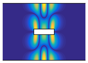
An example of invisibility-protected TMs (Evans et al. Reference Evans, Linton and Ursell1993; Davies & Parnovski Reference Davies and Parnovski1998; Groves Reference Groves1998; Linton & McIver Reference Linton and McIver1998; Linton et al. Reference Linton, McIver, McIver, Ratcliffe and Zhang2002) is given in figure 6, where a 2-D waveguide contains a zero-thickness plate parallel to the guide walls. In both short and long TMs, the coefficients of DMs in  $d3$ indicate the split of DMs, but in a way that is different from the
  $y$-symmetric split shown in figure 4(d,h). Here, the zero amplitudes of
  $k_n^+$ (
 $n=1,4,7\dots$) DMs in
  $d3$ indicate that this particular group of DMs in the guide are not involved in the TMs. Those DMs all have a node of vertical velocity at the plate position
  $y=1/3$, so they are not scattered by the plate. One may also say that the zero-thickness plate is invisible to those DMs in the guide. Since
  $k_2^{\pm }$ DMs do not have a node of vertical velocity within the guide,
  $k_2^{\pm }$ DMs are always scattered by a zero-thickness plate placed at any
  $y$-position in the guide. Therefore, the invisibility mechanism cannot protect an eigenmode from the radiation by
  $k_2^{\pm }$ DMs in the guide, and TMs protected by the invisibility mechanism alone exist only in the frequency range
  $0<\omega /{\rm \pi} <1$ where
  $k_2^{\pm }$ DMs in the guide are evanescent waves. The eigenfunction of the short TM in figure 6(a) is rather complex, whereas the long TM in figure 6(e) is simple and characterized by two standing waves in
  $d1$ and
  $d2$ formed by
  $k_1^{\pm }$ plane waves.

Figure 6. Trapped modes in a waveguide with a zero-thickness plate at  $y=1/3$: (a,e)
  ${\rm Re}(\,p)$ of short and long TMs (
 $L=0.3$,
  $\omega /{\rm \pi} =0.9870$;
  $L=10$,
  $\omega /{\rm \pi} =0.0961$); (b,f)
  ${\rm Re}(\,p)$ of
  $k_1^{\pm }$ cut-on DMs; (c,g)
  ${\rm Re}(\,p)$ of
  $k_2^{\pm }$ cut-off DMs; (d,h) modulus of mode coefficients of
  $k_n^+$ DMs in
  $d1$,
$d1$,  $d2$ and
  $d3$ in the TM eigenfunctions.
3.3. Symmetry–periodicity-protected TMs
Consider a 2-D waveguide containing  $N$ identical plates. If the plates are placed at the same
  $x$-position and at
  $y$-positions so that the heights of the parallel duct segments separated by the plates satisfy
  $H_1=H_{N+1}= H_j/2$ where
  $j=2, 3 \ldots N$, then an
  $N$-period section of an infinite array of equally spaced plates in the
  $y$-direction is formed. Figure 7 displays symmetry–periodicity-protected TMs (Utsunomiya & Eatock Taylor Reference Utsunomiya and Eatock Taylor1999; Porter & Evans Reference Porter and Evans1999; Linton & McIver Reference Linton and McIver2002) in an acoustic waveguide with two plates of thickness
  $T=1/8$. In this case, two patterns of TMs exist, i.e. the
  $y$-antisymmetric pattern shown in figure 7(a,i) and the
  $y$-symmetric pattern shown in figure 7(e,m). The mode coefficients of DMs in
  $d4$ shown in the third column of figure 7 indicate the decoupling of TMs of each pattern from a particular group of outgoing DMs in the waveguide. The
  $y$-antisymmetric TMs are decoupled from the outgoing
  $k_1^{\pm }$ but not
  $k_2^{\pm }$ DMs in the waveguide, thus the TM frequency range is
  $0<\omega /{\rm \pi} <1$. The
  $y$-symmetric TMs are decoupled from the outgoing
  $k_1^{\pm }$ and
  $k_2^{\pm }$ but not
  $k_3^{\pm }$ DMs in the waveguide, thus the TM frequency range is
  $0<\omega /{\rm \pi} <2$. In the frequency range all the TMs, i.e.
  $0<\omega /{\rm \pi} <2$, only
  $k_1^{\pm }$ plane waves are cut-on in the duct segments in the resonant region. The long TMs shown in figure 7(i,m) are simple and characterized by multiple standing waves in
  $d$1,
$d$1,  $d2$ and
  $d3$ formed by
  $k_1^{\pm }$ plane waves.

Figure 7. Trapped modes in a waveguide with two plates of thickness  $T=1/8$ which form a 2-period section of a vertically symmetric–periodic system: (a,i)
  ${\rm Re}(\,p)$ of short and long
  $y$-antisymmetric TMs (
 $L=0.3$,
  $\omega /{\rm \pi} =0.9737$;
  $L=10$,
  $\omega /{\rm \pi} =0.0957$); (e,m)
  ${\rm Re}(\,p)$ of short and long
  $y$-symmetric TMs (
 $L=0.3$,
  $\omega /{\rm \pi} =1.5830$;
  $L=10$,
  $\omega /{\rm \pi} =0.0973$); (b,f,j,n)
  ${\rm Re}(\,p)$ of
  $k_1^{\pm }$ cut-on DMs; (c,g,k,o)
  ${\rm Re}(\,p)$ of
  $k_2^{\pm }$ cut-off DMs; (d,h,l,p) modulus of mode coefficients of
  $k_n^+$ DMs in
  $d1$,
$d1$,  $d2$ and
  $d4$ in the TM eigenfunctions.
Symmetry–periodicity-protected TMs in an acoustic waveguide with three and four plates are shown in figure 8. In these two cases, there are respectively three and four patterns of TMs. In each pattern, the decoupled outgoing DMs in the waveguide, indicated by their mode coefficients, reveal the upper limit of TM frequency:  $\omega /{\rm \pi} <3$ (figure 8f) and
  $\omega /{\rm \pi} <4$ (figure 8n) in the three-plate and four-plate cases respectively. As in the two-plate case, only
  $k_1^{\pm }$ DMs are cut-on in the duct segments in the resonant region. The long TMs in figure 8 are also very simple and characterized by multiple standing waves formed by
  $k_1^{\pm }$ plane waves. Symmetry–periodicity-protected TMs in any high-frequency range (thus with any large number of cut-on DMs in the waveguide) can be obtained by increasing the periods
  $N$.
$N$.

Figure 8. Trapped modes in a waveguide with three plates ( $T=1/12$) and four plates (
 $T=1/16$) which form a 3- and 4-period section of a vertically symmetric–periodic system: (a–c)
  ${\rm Re}(\,p)$ of long TMs (
 $L=10$;
  $\omega /{\rm \pi} =0.09569$, 0.09777 and 0.09817) belonging to three different patterns and (d–f) modulus of mode coefficients of
  $k_n^+$ DMs in
  $d1$,
$d1$,  $d2$ and
  $d5$ in the TM eigenfunctions; (g–j)
  ${\rm Re}(\,p)$ of long TMs (
 $L=10$;
  $\omega /{\rm \pi} =0.09564$, 0.09782, 0.09846 and 0.09862) belonging to four different patterns and (k–n) modulus of mode coefficients of
  $k_n^+$ DMs in
  $d1$,
$d1$,  $d2$,
$d2$,  $d3$ and
  $d6$ in the TM eigenfunctions.
3.4. Accidental TMs
Figure 9 presents a simple and valuable example of accidental TMs, found previously by Xiong (Reference Xiong2016) in an  $x$-symmetric
  $y$-asymmetric cavity–waveguide system. Those TMs were later calculated and described in Dai (Reference Dai2021a), here, we re-calculate and collect them for the purpose of the comparison of various types of TMs. The mode coefficients of DMs in
  $d2$ shown in the third column of figure 9 indicate that the single outgoing cut-on DM (
 $k_{1}^+$) has a zero amplitude, i.e. zero radiation. Note that the number of decoupled DMs in the waveguide in this case is different from that in the common TMs described above: only one outgoing DM in the
  $\pm x$ directions in the waveguide is decoupled in this case, whereas a group of an infinite number of outgoing DMs (only one or a few of them are cut-on, however) are decoupled in the cases above. The second column of figure 9 shows that the TMs are characterized by two standing waves respectively formed by
  $k_{1}^{\pm }$ and
  $k_{2}^{\pm }$ DMs in the resonant region with total reflection at region boundaries. Different phase changes in total reflection can be observed:
  $k_{1}^{\pm }$ DMs seem always have a hard-wall reflection as shown in figure 9(b,g,l); for
  $k_{2}^{\pm }$ DMs, the total reflection is close to a pressure-release reflection in figure 9(h) but close to a hard-wall reflection in figure 9(m). Also note that the standing-wave characteristics in this case are different from those in the common TMs. First, two standing waves coexist in the cavity segment in this case, whereas there is no coexistence of standing waves in a single duct segment in the cases above. Second, cut-on DMs with two different wavelengths are involved in the resonant region in this case, whereas all cut-on DMs in the resonant region have the same wavelength in cases above.

Figure 9. Accidental TMs in a waveguide with a cavity with depth  $D=1.5$: (a,f,k)
  ${\rm Re}(\,p)$ of three TMs (
 $L=2.9025$ and
  $\omega /{\rm \pi} =0.6891$;
  $L=8.9333$ and
  $\omega /{\rm \pi} =0.6716$;
  $L=7.2356$ and
  $\omega /{\rm \pi} =0.9674$); (b,g,l)
  ${\rm Re}(\,p)$ of
  $k_1^{\pm }$ cut-on DMs; (c,h,m)
  ${\rm Re}(\,p)$ of
  $k_2^{\pm }$ cut-on DMs; (d,i,n)
  ${\rm Re}(\,p)$ of
  $k_3^{\pm }$ cut-off DMs; (e,j,o) modulus of mode coefficients of
  $k_n^+$ DMs in
  $d1$ and
  $d2$ in the TM eigenfunctions. Note that, in figures 9, 10 and 11, the calculated coefficients of the outgoing DMs decoupled by the accidental TM mechanism are of the order
  $10^{-8}$, which reduces as the number of DMs used in the calculations is increased.
Figure 10 displays accidental TMs in an open system with rotational symmetry. Those TMs are also characterized by two standing waves respectively formed by  $k_{1}^{\pm }$ and
  $k_{2}^{\pm }$ DMs in the resonant region. The TMs and their standing-wave components are either point antisymmetric in figure 10(a–c) or point symmetric in figure 10(e–g).

Figure 10. Accidental TMs in a system with rotational symmetry: (a,e)  ${\rm Re}(\,p)$ of two TMs (
 $L=1.3945$ and
  $\omega /{\rm \pi} =0.7171$;
  $L=5.6263$ and
  $\omega /{\rm \pi} =0.7109$); (b,f)
  ${\rm Re}(\,p)$ of
  $k_1^{\pm }$ cut-on DMs; (c,g)
  ${\rm Re}(\,p)$ of
  $k_2^{\pm }$ cut-on DMs; (d,h) modulus of mode coefficients of
  $k_n^+$ DMs in
  $d1$ and
  $d2$ in the TM eigenfunctions.
Figure 11 presents another example of accidental TMs, in which the travelling-wave components are more complex than those in figures 9 and 10. Those TMs were found previously by Duan et al. (Reference Duan, Koch, Linton and McIver2007) in a waveguide with a zero-thickness plate placed on the centreline of the guide. The accidental TM shown in figure 11(a), which is one of the Neumann TMs in the frequency range  $2<\omega /{\rm \pi} <3$ in figure 2 of Duan et al. (Reference Duan, Koch, Linton and McIver2007), might be understood as a result of co-protection. Over the frequency range
  $2<\omega /{\rm \pi} <3$,
  $k_n^{\pm }$ (
 $n=1,2,3$) DMs are cut-on in the waveguide
  $d3$; over the frequency range
  $2<\omega /{\rm \pi} <4$,
  $k_n^{\pm }$ (
 $n=1,2$) DMs are cut-on in
  $d1$ and
  $d2$. First, the
  $y$-symmetry of the system decouples
  $y$-antisymmetric TMs from the outgoing
  $k_n^{\pm }$ (
 $n=1,3$) DMs in the waveguide (the same as figure 4). Second, the coupled
  $k_1^{\pm }$ and
  $k_2^{\pm }$ standing waves in
  $d1$ and
  $d2$ decouple the TMs from the outgoing
  $k_{2}^{\pm }$ DMs in the waveguide. Note that, under the
  $y$-antisymmetric constraint for the DMs in
  $d1$ and
  $d2$, only the ratio between
  $k_1^{\pm }$ and
  $k_2^{\pm }$ standing waves in one of the two ducts is relevant to the decoupling of the outgoing
  $k_{2}^{\pm }$ DMs in the waveguide, which is essentially the same situation as that in figures 9 and 10. Accidental TMs due to such co-protection with the plate having a finite thickness
  $T$ are shown in figure 11(f,k). With a finite-thickness plate, the frequency range of those accidental TMs is not
  $2<\omega /{\rm \pi} <3$ but
  $2H/( H-T )<\omega /{\rm \pi} <3$, where the lower limit is required by the condition that there are two cut-on DMs in
  $d1$ and
  $d2$. So, if
  $2H/( H-T )>3$, i.e.
  $T>H/3$, those accidental TMs do not occur.

Figure 11. Accidental TMs in a waveguide with zero-thickness and finite-thickness ( $T=0.1$) plates on the centreline: (a,f,k)
  ${\rm Re}(\,p)$ of TMs (
 $L=1.2779$,
  $\omega /{\rm \pi} =2.1139$;
  $L=1.0819$,
  $\omega /{\rm \pi} =2.3416$;
  $L=2.0480$,
  $\omega /{\rm \pi} =2.9987$); (b,g,l)
  ${\rm Re}(\,p)$ of
  $k_1^{\pm }$ cut-on DMs; (c,h,m)
  ${\rm Re}(\,p)$ of
  $k_2^{\pm }$ cut-on DMs; (d,i,n)
  ${\rm Re}(\,p)$ of
  $k_3^{\pm }$ cut-off DMs; (e,j,o) modulus of mode coefficients of
  $k_n^+$ DMs in
  $d1$,
$d1$,  $d2$ and
  $d3$ in the TM eigenfunctions.
In all TMs above except figure 3, the number of cut-on DM pairs in the resonant region that participate in the eigenfunctions is one (or more than one, as in figure 8a,b,g) larger than the number of outgoing cut-on DMs in the waveguide, which gives just the right amount of freedom (or sufficient freedom) to cancel the radiation (Linton & McIver Reference Linton and McIver2007). However, for example, if the plate in figures 4 and 11 is moved slightly off the centreline, the number of cut-on DM pairs in the resonant region can remain unchanged in a slightly changed frequency range but the TMs disappear. Therefore, we need to understand why in those scenarios the cut-on DM pairs in the resonant region cannot underpin a TM by mutual cancellation in radiation (see the phase compensation in (4.46) thanks to  $k_1^{\pm } \neq\, k_2^{\pm }$).
4. Travelling-wave analysis of the eigenfunctions of long TMs ( $L \gg 1$)

With the TM definition in § 2, this section investigates and compares the mechanisms of TMs by analysing why and how the travelling-wave components of the eigenfunction can satisfy the eigenmode condition (loop magnitude and phase constraints for closure) and the wave-trapping condition (loop zero-radiation condition) simultaneously. To simplify the task, inspired by the asymptotic equation (2.1) and the visually simple eigenfunctions of long TMs in § 3, we analyse long TMs with  $L \gg 1$. In TMs calculated above with
  $L=10$, in general,
  $\mathrm {exp} ( \mp \mathrm {i} k_n^{\pm } L) < 10^{-20}$ for cut-off DMs in the resonant region. In this section, we assume
  $\mathrm {exp} ( \mp \mathrm {i} k_n^{\pm } L) =0$ for cut-off DMs. First, the assumption reduces the analysis of
  $N_{t}$ loops to
  $N_{{cut\text -on}}$ loops, where
  $N_{t}$ is the number of all DMs in the resonant region and
  $N_{{cut\text -on}}$ is the number of cut-on DMs. Second, it means that in the analysis of wave scattering at the region boundaries, the only incident waves are
  $k_n^{\pm }$ cut-on DMs in the resonant region.
In a 2-D hard-walled duct with DMs in the  $\pm x$ directions, the transmitted acoustic power can be obtained by integrating the time-averaged axial intensity,
  $\langle I_x \rangle =(\kern0.7pt pu^*+p^*u ) /4 = \mathrm {Re} (\kern0.7pt pu^*) /2$, where
  $I_x$ and
  $u$ are intensity and velocity in the
  $x$ direction and the stars denote complex conjugates, over the duct cross-section (Rienstra & Hirschberg Reference Rienstra and Hirschberg2021)
 \begin{equation} \mathcal{P} = \frac{\rm \pi}{\omega} \sum_{n=1}^N \big[\mathrm{Re} \big( k_n^+ \big) \big( \big| C_n^+ \big| ^2- \big| C_n^- \big| ^2 \big) +2 \mathrm{Im} \big( k_n^+ \big) \mathrm{Im} \big( E_n^{+*}E_n^- \big) \big] ,\end{equation}
where  $N$ is the number of DMs in the
  $\pm x$ directions. The wavenumbers of cut-on and cut-off DMs are respectively purely real and imaginary at a real frequency and
  $k_n^+ =-k_n^-$. Here,
  $C_n^{\pm }$ and
  $E_n^{\pm }$ respectively denote the mode coefficients of cut-on and cut-off DMs. Equation (4.1) reveals energy transmission due to not only cut-on DMs but also the interaction between a pair of
  $k_n^+$ and
  $k_n^-$ cut-off DMs. Note that, for the energy related expression, the profiles of DMs are normalized by modal energy
 \begin{equation} P_n(y) =
\frac{\mathrm{cos}[ (n-1){\rm \pi} y/H_j]}{
\sqrt{[1/2]_{n{\neq}1}H_j } },
\end{equation}
\begin{equation} P_n(y) =
\frac{\mathrm{cos}[ (n-1){\rm \pi} y/H_j]}{
\sqrt{[1/2]_{n{\neq}1}H_j } },
\end{equation}
where  $H_j$ is duct height,
  $n=1,2,3\ldots$.
In the eigenfunctions, the wave scattering at the right end of TMs is sketched in figure 12. Here,  $C_n^{\pm }$ denotes the mode coefficients of cut-on DMs in the
  $\pm x$ directions in the resonant region,
  $B_n^+$ denotes the mode coefficients of outgoing cut-on DMs in the right semi-infinite waveguide. Under the long TM assumption, the only incident waves onto the scattering interface are one or a few cut-on DMs, denoted by the blue arrows. No pairs of
  $k_n^+$ and
  $k_n^-$ cut-off DMs are present on both the left and the right sides of the scattering interface. Therefore, the term
 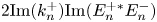 $2 \mathrm {Im} ( k_n^+ ) \mathrm {Im} ( E_n^{+*}E_n^- )$ in (4.1) associated with evanescent pairs can be disregarded. Then, the time-averaged energy conservation in a vanishingly small volume enclosing the scattering interface gives
 \begin{equation} \sum_{n=1}^{N_C} k_{n,C}^+ \big( \big| C_n^+ \big| ^2- \big| C_n^- \big| ^2 \big)= \sum_{n=1}^{N_B} k_{n,B}^+ \left| B_n^+ \right| ^2 , \end{equation}
where  $N_C$ and
  $N_B$ are the number of cut-on DMs involved on the left and right sides of the scattering interface,
  $k_{n,C}^+$ and
  $k_{n,B}^+$ are the wavenumbers of those cut-on DMs.

Figure 12. Sketches of wave scattering at the right end of long TMs ( $L \gg 1$). (a–f) Respectively correspond to figures 3, 4, 6, 7, 9 and 11. Blue arrows: incident waves; black arrows: scattered waves. Straight-line arrows: cut-on DMs; polyline arrows: cut-off DMs; arrows with an additional short line: cut-on DMs with zero amplitude.
4.1. Symmetry-protected TMs
Figure 12(a) corresponds to the TMs in figure 3. For  $D=2H$, they happen under necessary conditions that only
  $k_{1}^{\pm }$ DMs are cut-on in
  $d2$ and only
  $k_1^{\pm }$ and
  $k_2^{\pm }$ DMs are cut-on in
  $d1$. For a larger
  $D$, the second condition is that only one pair of
  $y$-antisymmetric
  $k_n^{\pm }$ DMs is cut-on in
  $d1$. In the decomposed eigenfunction, the only incident wave on the interface is
  $k_2^+$ DM in
  $d1$. Then, the
  $y$-symmetry of the system ensures
 \begin{equation} \left| B_1^+ \right| =0,\end{equation}
and
 \begin{equation} \left| C_1^- \right| =0.\end{equation}
With (4.4) and (4.5), the expression of energy conservation (4.3) gives
 \begin{equation} \left| \frac{C_2^-}{C_2^+} \right|=1,\end{equation}
meaning that  $k_2^+$ DM is totally reflected. Total reflection of
  $k_2^-$ DM and zero radiation to infinity also happen at the left end. Therefore, the loop magnitude constraint and the loop zero-radiation condition are satisfied by a
  $k_2^{\pm }$-loop of DMs in
  $d1$. For an
  $x$-symmetric system, the loop phase constraint (2.3) that selects the TM frequency for a given
  $L$ can be reformed
 \begin{equation} \mathrm{arg}\bigg( \frac{C_2^-}{C_2^+} \bigg) - k_2^+L =-m {\rm \pi},\end{equation}
where  $m$ is an integer. Equation (4.7) means that the phase change of half of the loop is an integer multiple of
  ${\rm \pi}$. Even and odd values of
  $m$ respectively correspond to
  $x$-symmetric and
  $x$-antisymmetric eigenmodes.
The interface scattering matrix, which relates the outgoing waves to the incoming waves on the interface, is numerically calculated by matching DMs in  $d1$ and
  $d2$ (the number of DMs used in the matching is the same as that in the calculations in § 3). From the interface scattering matrix, the value of
  $C_2^-/C_2^+$ is extracted, as shown in figure 13(a,b). The calculated modulus agrees with (4.6). The phase change varies continuously with frequency in such a way:
 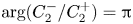 $\mathrm {arg}( C_2^-/C_2^+ ) = {\rm \pi}$ and
  $\mathrm {arg}( C_2^-/C_2^+ ) \approx 0$ respectively at the lower and upper limits of the frequency range. An analysis of the phase change in total reflection at waveguide discontinuities is given in Appendix A. With the calculated
  $\mathrm {arg}( C_2^-/C_2^+ )$, (4.7) gives the
  $L$–
$L$– $\omega$ relation in figure 13(c). From the comparison for
  $m=0$ and
  $m=1$ branches, we can see that the lines obtained from (4.7) predict TMs well, except when
  $L$ is small.


Figure 12(b) corresponds to the TMs in figure 4, which happen under necessary conditions that only  $k_{1}^{\pm }$ DMs are cut-on in
  $d3$ and only
  $k_{1}^{\pm }$ DMs are cut-on in
  $d1$ and
  $d2$. The scattering relation of cut-on DMs is written as
 \begin{equation}
\left(\begin{array}{@{}c@{}} C_1^- \\
C_2^- \\ B_1^+ \end{array}\right) =
\left[\begin{array}{@{}cc@{}} R_{11} & R_{12} \\ R_{21} &
R_{22} \\ T_{11} & T_{12} \end{array}\right]
\left(\begin{array}{@{}c@{}} C_1^+ \\
C_2^+ \end{array}\right)\!.
\end{equation}
\begin{equation}
\left(\begin{array}{@{}c@{}} C_1^- \\
C_2^- \\ B_1^+ \end{array}\right) =
\left[\begin{array}{@{}cc@{}} R_{11} & R_{12} \\ R_{21} &
R_{22} \\ T_{11} & T_{12} \end{array}\right]
\left(\begin{array}{@{}c@{}} C_1^+ \\
C_2^+ \end{array}\right)\!.
\end{equation}
The  $y$-symmetry of the system ensures
 \begin{equation} T_{11} =T_{12},\quad R_{11} = R_{22}, \quad R_{12} = R_{21}. \end{equation}
Therefore, if the incident waves satisfy
 \begin{equation} C_1^+=- C_2^+, \end{equation}
then
 \begin{equation} B_1^+=T_{11}C_1^++ T_{12}C_2^+=0, \end{equation}
understood as meaning that  $k_1^+$ DM in
  $d1$ and
  $k_1^+$ DM in
  $d2$ cancel each other in transmission to
  $k_1^+$ DM in
  $d3$. Due to (4.9b,c), the incidence combination (4.10) also leads to
 \begin{equation} \frac{C_1^-}{C_1^+} =R_{11} + R_{12} \frac{C_2^+}{C_1^+} =R_{21} \frac{C_1^+}{C_2^+} + R_{22}= \frac{C_2^-}{C_2^+}. \end{equation}
With (4.11) and (4.12), the expression of energy conservation (4.3) gives
 \begin{equation} \left| \frac{C_1^-}{C_1^+} \right| = \left| \frac{C_2^-}{C_2^+} \right| =1. \end{equation}
 Firstly, (4.13) indicates that the two  $k_1^+$ DMs in respectively
  $d1$ and
  $d2$ both have total reflection at the interface, i.e. the magnitudes of the DMs are unvarying in reflection. At real frequencies, the magnitudes of
  $k_1^{\pm }$ cut-on DMs are also unvarying in propagation. Secondly, (4.12) indicates that the phase changes of the two
  $k_1^+$ DMs are the same in reflection. The phase changes of the two
  $k_1^+$ DMs in propagation from the left to the right end (or of the two
  $k_1^-$ DMs in the reverse direction) are also the same for any
  $L$, owing to the same wavenumber. Therefore, once the amplitude ratio between the two
  $k_1^{\pm }$ loops in respectively
  $d1$ and
  $d2$ is prescribed as in (4.10), the loop magnitude constraint and the loop zero-radiation condition are satisfied. Although two loops are involved,
  $k_1^{\pm }$ loops in
  $d1$ and
  $d2$ share the same phase constraint owing to the equal wavenumber and the equal phase change in boundary reflection
 \begin{equation} \mathrm{arg}\left( \frac{C_j^-}{C_j^+} \right) - k_1^+L =-m {\rm \pi},\end{equation}
where  $m$ is an integer,
  $j=1$ or 2. Even and odd values of
  $m$ respectively correspond to
  $x$-symmetric and
  $x$-antisymmetric TMs.
The interface scattering matrix is numerically calculated by matching DMs in  $d1$,
$d1$,  $d2$ and
  $d3$, from which the value of
  $C_1^-/C_1^+$ (or
  $C_2^-/C_2^+$) is extracted, as shown in figure 14(a,b). With the calculated
  $\mathrm {arg}( C_1^-/C_1^+ )$, (4.14) gives the
  $L$–
$L$– $\omega$ relation in figure 14(c). From the comparison for
  $m=0$ and
  $m=1$ branches, i.e. Parker's
  $\beta$- and
  $\alpha$-modes (Parker Reference Parker1966), we can see that the lines from (4.14) predict TMs well.


4.2. Invisibility-protected TMs
Figure 12(c) corresponds to the TMs in figure 6, which happen under necessary conditions that only  $k_{1}^{\pm }$ DMs are cut-on in
  $d3$ and only
  $k_{1}^{\pm }$ DMs are cut-on in
  $d1$ and
  $d2$. The scattering relation of cut-on DMs is written as
 \begin{equation} \left(\begin{array}{@{}c@{}} C_1^- \\ C_2^- \\ B_1^+ \end{array}\right) = \left[\begin{array}{@{}cc@{}} R_{11} & R_{12} \\ R_{21} & R_{22} \\ T_{11} & T_{12} \end{array}\right] \left(\begin{array}{@{}c@{}} C_1^+ \\ C_2^+ \end{array}\right)\!. \end{equation}
Because the interface scattering matrix is an invariant to the combination of incident waves, the values of or the relations between some elements of the scattering matrix can be extracted from particular incidence combinations. Imagine  $k_1^-$ DM incoming from
  $d3$, then the zero-thickness plate does not scatter the plane wave. So,
  $k_1^-$ DM propagates in the
  $-x$-direction in the waveguide as if the zero-thickness plate was not present. Reversing the direction of wave propagation gives a second solution (also with no evanescent waves being scattered)
 \begin{equation} \left. \begin{array}{l@{}} C_1^+=C_2^+=B_1^+,\\ C_1^-=C_2^-=0. \end{array}\right\} \end{equation}
Such a solution leads to
 \begin{equation} \left. \begin{array}{l@{}} T_{11} + T_{12}=1,\\ R_{11} + R_{12}=0,\\ R_{21} + R_{22}=0. \end{array}\right\} \end{equation}
Tracing the total transmission and zero reflection of mass fluxes incoming from  $d1$ and
  $d2$ (mass fluxes can be easily traced here because there are no evanescent waves being scattered in this particular situation) gives
 \begin{equation} \left. \begin{array}{l@{}} T_{11} /T_{12}=H_1/H_2, \\ H_1 R_{11}+H_2 R_{21}=0, \\ H_1 R_{12}+H_2 R_{22} =0, \end{array}\right\} \end{equation}
where  $H_1$ and
  $H_2$ are the heights of
  $d1$ and
  $d2$.
$d2$.
Now, we consider the wave scattering sketched in 12(c). According to (4.18), if the incident waves satisfy
 \begin{equation} \frac{C_1^+ }{C_2^+} =- \frac{H_2}{H_1}, \end{equation}
then
 \begin{equation} B_1^+=T_{11}C_1^++ T_{12}C_2^+=0. \end{equation}
Equations (4.18) and (4.19) also lead to
 \begin{equation} \frac{C_1^-}{C_1^+} =R_{11} + R_{12} \frac{C_2^+}{C_1^+} =R_{21} \frac{C_1^+}{C_2^+} + R_{22}= \frac{C_2^-}{C_2^+}. \end{equation}
We can see that this case is very similar to the second case in § 4.1, except for the different amplitude ratios of  $k_1^{\pm }$ loops prescribed in (4.10) and (4.19). For this case, the same equations as (4.13) and (4.14) can be obtained. We skip them but plot the
  $C_1^-/C_1^+$ (or
  $C_2^-/C_2^+$) as a function of frequency and the
  $L$–
$L$– $\omega$ relation in figure 15.


4.3. Symmetry–periodicity-protected TMs
Figure 12(d) corresponds to the TMs in figure 7, which happen under necessary conditions that only  $k_{1}^{\pm }$ DMs are cut-on in
  $d4$ in the
  $y$-antisymmetric pattern of TMs whereas only
  $k_1^{\pm }$ and
  $k_2^{\pm }$ DMs are cut-on in
  $d4$ in the
  $y$-symmetric pattern of TMs, and in both patterns only
  $k_{1}^{\pm }$ DMs are cut-on in
  $d1$,
$d1$,  $d2$ and
  $d3$. The scattering relation of cut-on DMs is written as
 \begin{equation} \left(\begin{array}{@{}c@{}} C_1^- \\ C_2^- \\ C_3^- \\ B_1^+ \\ B_2^+ \end{array}\right) = \left[\begin{array}{@{}ccc@{}} R_{11} & R_{12} & R_{13} \\ R_{21} & R_{22} & R_{23} \\ R_{31} & R_{32} & R_{33} \\ T_{11} & T_{12} & T_{13} \\ T_{21} & T_{22} & T_{23} \end{array}\right] \left(\begin{array}{@{}c@{}} C_1^+ \\ C_2^+ \\ C_3^+ \end{array}\right)\!. \end{equation}
The  $y$-symmetry of the system ensures the following relations of transmission and reflection:
 $$\begin{gather} T_{11}=T_{13}, \quad T_{21}=-T_{23}, \quad T_{22}=0, \end{gather}$$
 $$\begin{gather}R_{11}=R_{33}, \quad R_{13}=R_{31}, \quad R_{12}=R_{32}, \quad R_{21}=R_{23}. \end{gather}$$
Consider an incidence combination  $C_1^+ = -C_2^+ = C_3^+$, the resulting field is symmetric about the waveguide centreline
  $y=H/2$. Therefore, placing a zero-thickness infinite-length plate at
  $y=H/2$ does not change the field. The plate divides the system into two identical sub-systems. In each
  $y$-symmetric sub-system, the scattering of the
  $y$-antisymmetric incidence is the same as analysed in § 4.1. Therefore
 \begin{equation} \frac{C_1^-}{C_1^+} = \frac{C_2^-}{C_2^+} = \frac{C_3^-}{C_3^+}, \end{equation}
and
 \begin{equation} \left|\frac{C_1^-}{C_1^+}\right| = \left|\frac{C_2^-}{C_2^+}\right| = \left|\frac{C_3^-}{C_3^+}\right| =1. \end{equation}
Also,  $B_1^+=0$ under the incidence combination
  $C_1^+ = -C_2^+ = C_3^+$ gives
 \begin{equation} T_{11}- T_{12}+T_{13}=0. \end{equation}
Now, we consider the wave scattering in long TMs sketched in 12(d). According to the transmission relations in (4.23a–c) and (4.27), if the incident waves satisfy
 \begin{equation} \left. \begin{array}{l@{}} C_1^++ 2 C_2^++ C_3^+=0, \\ C_1^+- C_3^+=0, \end{array}\right\} \end{equation}
then the net transmissions to both  $k_{1}^+$ and
  $k_{2}^+$ DMs in
  $d4$ are zero
 \begin{equation} \left. \begin{array}{l@{}} B_1^+=T_{11}C_1^++ T_{12}C_2^++ T_{13}C_3^+=0, \\ B_2^+=T_{21}C_1^++ T_{22}C_2^++ T_{23}C_3^+=0. \end{array}\right\} \end{equation}
The only solution of (4.28) for the ratios between DM coefficients is
 \begin{equation} C_1^+= -C_2^+= C_3^+, \end{equation}
which corresponds to the reflection relations in (4.25) and (4.26) and the  $y$-symmetric patten of TMs. To have zero net transmission to only
  $k_{1}^+$ DM in
  $d4$, another solution, associated with a
  $y$-antisymmetric incidence and the
  $y$-antisymmetric patten of TMs, is
 \begin{equation} C_1^+= -C_3^+, \quad C_2^+=0. \end{equation}
For the incidence combination (4.31a,b), (4.24a,b) leads to
 \begin{equation} \frac{C_1^-}{C_1^+} =R_{11} + R_{13} \frac{C_3^+}{C_1^+} = R_{31} \frac{C_1^+}{C_3^+} + R_{33} = \frac{C_3^-}{C_3^+}. \end{equation}
Then, with  $B_1^+=0$ and (4.32), if
  $k_2^+$ DM in
  $d4$ is cut-off, (4.3) gives
 \begin{equation} \left|\frac{C_1^-}{C_1^+}\right| = \left|\frac{C_3^-}{C_3^+}\right| =1. \end{equation}
 This case is also similar to the second case in § 4.1 in the sense that, once  $k_1^{\pm }$ loops in
  $d$1,
$d$1,  $d2$ and
  $d3$ have the amplitude ratio as prescribed in (4.30) or (4.31a,b), the loop magnitude constraint and the loop zero-radiation condition are satisfied. For each TM pattern,
  $k_1^{\pm }$ loops in
  $d1$,
$d1$,  $d2$ and
  $d3$ share the same phase constraint owing to the equal wavenumber and the equal phase change in boundary reflection
 \begin{equation} \mathrm{arg}\bigg( \frac{C_j^-}{C_j^+} \bigg) - k_1^+L=-m {\rm \pi},\end{equation}
where  $m$ is an integer,
  $j=1$ or 3 for the
  $y$-antisymmetric pattern and
  $j=1$ or 2 or 3 for the
  $y$-symmetric pattern. The numerically calculated reflection coefficients and the
  $L$–
$L$– $\omega$ relation from (4.34) are plotted in figure 16. The
  $L$–
$L$– $\omega$ relation is verified by the TMs shown in figure 7 and the TMs calculated with
  $L=5$.

Figure 16. (a,b) Modulus and argument of  $C_1^-/C_1^+$ in the interface scattering sketched in figure 12(d). Thin and thick lines:
  $y$-symmetric and
  $y$-antisymmetric pattens with the incidence combinations (4.30) and (4.31a,b). (c) Solid and dashed lines:
  $L$–
$L$– $\omega$ relation from (4.34) with
  $m$ being even and odd. Symbols: TMs; squares: TMs shown in figure 7.
4.4. Accidental TMs
Figure 12(e) corresponds to the accidental TMs in figure 9, which happen under necessary conditions that only  $k_{1}^{\pm }$ DMs are cut-on in
  $d2$ and only
  $k_1^{\pm }$ and
  $k_2^{\pm }$ DMs are cut-on in
  $d1$. The scattering relation of cut-on DMs is written as
 \begin{equation} \left(\begin{array}{@{}c@{}} C_1^- \\ C_2^- \\ B_1^+ \end{array}\right) = \left[\begin{array}{@{}cc@{}} R_{11} & R_{12} \\ R_{21} & R_{22} \\ T_{11} & T_{12} \end{array}\right] \left(\begin{array}{@{}c@{}} C_1^+ \\ C_2^+ \end{array}\right)\!. \end{equation}
If the incident waves satisfy
 \begin{equation} \frac{C_1^+}{C_2^+} =- \frac{T_{12}}{T_{11}}, \end{equation}
then
 \begin{equation} B_1^+=0. \end{equation}
The incident combination (4.36) also leads to
 \begin{equation} \left. \begin{array}{l@{}} \displaystyle \dfrac{C_1^-}{C_1^+} = R_{11} - R_{12}\dfrac{T_{11}}{T_{12}}, \\[12pt] \displaystyle \dfrac{C_2^-}{C_2^+} = R_{22} - R_{21}\dfrac{T_{12}}{T_{11}}. \end{array}\right\} \end{equation}
With (4.37), the expression of energy conservation (4.3) gives
 \begin{equation} k_1^+ \big( \big| C_1^+ \big| ^2 - \big| C_1^- \big| ^2 \big) +k_2^+ \big( \big| C_2^+ \big| ^2 - \big| C_2^- \big| ^2 \big) =0, \end{equation}
which can be written equivalently as
 \begin{equation} k_1^+ \big( \big| T_{12} \big| ^2 - \big| R_{11}T_{12}- R_{12}T_{11} \big| ^2 \big) +k_2^+ \big( \big| T_{11} \big| ^2 - \big| R_{22}T_{11}- R_{21}T_{12} \big| ^2 \big) =0. \end{equation}
For the incidences of only one of  $k_1^+$ and
  $k_2^+$ DMs in
  $d1$, (4.3) gives
 \begin{equation} \left. \begin{array}{l@{}} \displaystyle k_1^+= k_1^+ \left| R_{11} \right| ^2 + k_2^+ \left| R_{21} \right| ^2 + k_r^+ \left| T_{11} \right| ^2, \\ \displaystyle k_2^+= k_1^+ \left| R_{12} \right| ^2 + k_2^+ \left| R_{22} \right| ^2 + k_r^+ \left| T_{12} \right| ^2, \end{array}\right\} \end{equation}
and for the incidence combinations  $C_1^+/C_2^+ = - R_{22}/R_{21}$ and
  $C_1^+/C_2^+ = - R_{12}/R_{11}$, (4.3) gives
 \begin{equation} \left.
\begin{array}{l@{}} \displaystyle k_1^+ \big( \big|
R_{22} \big| ^2 - \big| R_{11}R_{22}- R_{12}R_{21}
\big| ^2 \big) +k_2^+ \big| R_{21} \big| ^2 = k_r^+
\big| R_{22}T_{11}- R_{21}T_{12} \big| ^2, \\
\displaystyle k_1^+ \big| R_{12} \big| ^2 + k_2^+ \big(
\big| R_{11} \big| ^2 - \big| R_{11}R_{22}-
R_{12}R_{21} \big| ^2 \big) = k_r^+ \left|
R_{11}T_{12}- R_{12}T_{11} \right| ^2. \end{array}\right\}
\end{equation}
\begin{equation} \left.
\begin{array}{l@{}} \displaystyle k_1^+ \big( \big|
R_{22} \big| ^2 - \big| R_{11}R_{22}- R_{12}R_{21}
\big| ^2 \big) +k_2^+ \big| R_{21} \big| ^2 = k_r^+
\big| R_{22}T_{11}- R_{21}T_{12} \big| ^2, \\
\displaystyle k_1^+ \big| R_{12} \big| ^2 + k_2^+ \big(
\big| R_{11} \big| ^2 - \big| R_{11}R_{22}-
R_{12}R_{21} \big| ^2 \big) = k_r^+ \left|
R_{11}T_{12}- R_{12}T_{11} \right| ^2. \end{array}\right\}
\end{equation}
Note that  $k_r^+$ denotes the wavenumber of the involved cut-on DM in
  $d2$. In the case in figure 9
  $k_r^+=k_1^+$, whereas in figure 22(a,b)
  $k_r^+$ is unequal to the incident wavenumbers in
  $d1$. Combining (4.41) and (4.42), and the following reciprocity relation for wave reflection at the waveguide discontinuity (Cho Reference Cho1980):
 \begin{equation} k_1^+ R_{12} = k_2^+ R_{21}, \end{equation}
gives
 \begin{equation} k_1^+ \big( \big|
T_{12} \big| ^2 - \big| R_{11}T_{12}- R_{12}T_{11}
\big| ^2 \big) = k_2^+ \big( \big| T_{11} \big| ^2
- \big| R_{22}T_{11}- R_{21}T_{12} \big| ^2 \big)\!.
\end{equation}
\begin{equation} k_1^+ \big( \big|
T_{12} \big| ^2 - \big| R_{11}T_{12}- R_{12}T_{11}
\big| ^2 \big) = k_2^+ \big( \big| T_{11} \big| ^2
- \big| R_{22}T_{11}- R_{21}T_{12} \big| ^2 \big)\!.
\end{equation}Relations (4.40) and (4.44) lead to
 \begin{equation} \left|\frac{C_1^-}{C_1^+}\right| = \left|\frac{C_2^-}{C_2^+}\right| =1. \end{equation}
So we have proved total reflection of each DM, i.e. no energy interchange between  $k_{1}^{\pm }$ DMs and
  $k_{2}^{\pm }$ DMs, in the two-wave coupled total reflection.
The amplitude ratio of  $k_1^+$ and
  $k_2^+$ DMs (4.36) ensures the zero net transmission (4.37) and the total reflection of each of
  $k_1^+$ and
  $k_2^+$ DMs (4.45) at the right end. Due to the total reflection of each of
  $k_1^+$ and
  $k_2^+$ DMs and the real wavenumbers of cut-on DMs at real frequencies, the modulus of the amplitude ratio of
  $k_1^-$ and
  $k_2^-$ DMs at the left end is the same as that given by (4.36), So, if the following two loop phase constraints are satisfied:
 \begin{equation} \left.
\begin{array}{l@{}} \displaystyle \mathrm{arg}\bigg(
\dfrac{C_1^-}{C_1^+} \bigg) - k_1^+L =- m_1 {\rm \pi}, \\[12pt]
\displaystyle \mathrm{arg}\bigg( \dfrac{C_2^-}{C_2^+}
\bigg) - k_2^+L =- m_2 {\rm \pi}, \end{array}\right\}
\end{equation}
\begin{equation} \left.
\begin{array}{l@{}} \displaystyle \mathrm{arg}\bigg(
\dfrac{C_1^-}{C_1^+} \bigg) - k_1^+L =- m_1 {\rm \pi}, \\[12pt]
\displaystyle \mathrm{arg}\bigg( \dfrac{C_2^-}{C_2^+}
\bigg) - k_2^+L =- m_2 {\rm \pi}, \end{array}\right\}
\end{equation}
then zero radiation at both ends and of the two loops is ensured, where  $m_1$ and
  $m_2$ are integers and they both are even or odd for the
  $x$-symmetric system in figure 9 so that
  $k_1^{\pm }$ and
  $k_2^{\pm }$ loops have the same
  $x$-symmetry. The difference between the phase changes of the two loops in reflection is compensated by the propagation, thanks to
  $k_1^{\pm } \neq\, k_2^{\pm }$. With total reflection at both ends, the magnitude constraint of the two loops is also satisfied, at real frequencies.
Now, the difference between the mechanisms of common and accidental TMs can be understood by comparing how the loop zero-radiation condition is satisfied in the two situations. In common TMs that involve multiple propagating-wave loops, loop zero radiation is ensured alone by the particular amplitude ratio between the loops and it is independent of the single loop phase constraint that selects  $\omega _{TM}$ as a continuous function of
  $L$, due to the geometrical properties of the systems. On the other hand, loop zero radiation in accidental TMs depends on not only the amplitude ratio between the propagating-wave loops but also the loop phase constraints and there are two phase constraints. Only at the crossing points of the two phase constraints can zero-radiation loops be ensured, which is the reason for the discrete appearance of accidental TMs in the
  $L$–
$L$– $\omega$ two-parameter space.
To illustrate (4.46), the incidence combination  $C_1^+ /C_2^+$ in (4.36) and the reflection coefficients
  $C_1^- /C_1^+$ and
  $C_2^- /C_2^+$ in (4.38) are calculated by modal matching at the interface, as shown in figure 17(a,b). The two phase constraints in (4.46) lead to two groups of
  $L$–
$L$– $\omega$ lines. For the
  $x$-symmetric system in figure 9,
  $x$-symmetric and
  $x$-antisymmetric TMs happen at the crossing points of the two groups of lines with
  $m_1$ and
  $m_2$ both being even and odd. The squares in figure 17(c) indicate that (4.46) is accurate for all accidental TMs of the
  $x$-symmetric system. For the point-symmetric system in figure 10, point-symmetric and point-antisymmetric TMs, two of which are denoted by the diamonds in figure 17(c), happen at the crossing points of the two groups of
  $L$–
$L$– $\omega$ lines from (4.46) with
  $m_1$ and
  $m_2$ having opposite parities so that
  $k_1^{\pm }$ and
  $k_2^{\pm }$ loops have the same point symmetry.

Figure 17. (a,b) Modulus and argument of  $C_1^-/C_1^+$ and
  $C_2^-/C_2^+$ in the interface scattering sketched in figure 12(e) with the incidence combination (4.36). (c) Solid and dashed lines:
  $L$–
$L$– $\omega$ relation from (4.46) with
  $m_{1,2}$ being even and odd. Thick and line lines:
  $k_1^{\pm }$ and
  $k_2^{\pm }$ loops. Squares: accidental TMs of the system in figure 9; diamonds: accidental TMs shown in figure 10(a,e).
Figure 12(f) corresponds to the accidental TMs in figure 11(f,k), which happen under necessary conditions that  $k_n^{\pm }$ (
 $n=1,2,3$) DMs are cut-on in
  $d3$ and
  $k_n^{\pm }$ (
 $n=1,2$) DMs are cut-on in
  $d1$ and
  $d2$. In figure 12(f),
  $C_{1,2}^{\pm }$ denote the amplitudes of
  $k_{1,2}^{\pm }$ DMs in
  $d1$,
$d1$,  $C_{3,4}^{\pm }$ denote the amplitudes of
  $k_{1,2}^{\pm }$ DMs in
  $d2$ and
  $B_{1,2,3}^+$ denote the amplitudes of
  $k_{1,2,3}^+$ DMs in
  $d3$. We may understand the TMs as the result of co-protection: the
  $y$-symmetry protection as in § 4.1 and the most simple accidental TM mechanism above. If the incident waves satisfy
 \begin{equation} C_1^+=-C_3^+ \quad \mbox{and}\quad C_2^+=C_4^+, \end{equation}
then
 \begin{equation} B_1^+=B_3^+=0, \end{equation}
owing to the  $y$-symmetry of the system. If the incident waves also satisfy
 \begin{equation} \frac{C_1^+}{C_2^+} =- \frac{T_{22}}{T_{21}}, \end{equation}
where  $T_{21}$ and
  $T_{22}$ respectively denote the transmission from
  $k_1^+$ and
  $k_2^+$ DMs in
  $d1$ to
  $k_2^+$ DM in
  $d3$, then
 \begin{equation} B_2^+=0. \end{equation}
In a similar way, we can obtain total reflection as (4.45) and two phase constraints as (4.46) for this case. The incidence combination  $C_1^+ /C_2^+$ and the reflection coefficients
  $C_1^- /C_1^+$ and
  $C_2^- /C_2^+$ are shown in figure 18(a,b), and the graphical solution of TM locations in the
  $L$–
$L$– $\omega$ two-parameter space is verified by the two squares in figure 18(c).

Figure 18. (a,b) Modulus and argument of  $C_1^-/C_1^+$ and
  $C_2^-/C_2^+$ in the interface scattering sketched in figure 12(f) with the incidence combination (4.47a,b) and (4.49). (c) Solid and dashed lines:
  $L$–
$L$– $\omega$ relation from (4.46) with
  $m_{1,2}$ being even and odd. Thick and line lines:
  $k_1^{\pm }$ and
  $k_2^{\pm }$ loops. Squares: accidental TMs shown in figure 11(f,k).
5. Exclusion of modal degeneracy, avoided crossing and resonance-width bifurcation from TM-causing mechanism
Consider the open cavity–waveguide systems in figures 9 and 10 being closed by straight walls at  $x=0$ and
  $x=L$. In the closed rectangular cavity, each pair of
  $k_n^{\pm }$ cut-on DMs between
  $x=0$ and
  $x=L$ forms a loop that is independent from the others in propagation and reflection. The real eigenfrequency of each eigenmode is selected by the loop phase constraint (2.3) with hard-wall boundary reflection (
 $R_0 =R_L=1$). For some values of
  $L$, if the phase constraints of
  $k_{n_1}^{\pm }$ and
  $k_{n_2}^{\pm }$ loops (
 $k_{n_1}^{\pm } \neq\, k_{n_2}^{\pm }$) are satisfied at the same frequency
 \begin{equation} \left. \begin{array}{l@{}} k_{n_1}^+L = m_1 {\rm \pi}, \\ k_{n_2}^+L = m_2 {\rm \pi}, \end{array}\right\} \end{equation}
where  $m_1$ and
  $m_2$ are integers, the two eigenmodes of the closed cavity are called degenerate (McIntosh Reference McIntosh1959; Greenberg Reference Greenberg1966; Morse & Ingard Reference Morse and Ingard1987). Comparing (4.46) with (5.1) reveals a common feature between accidental TM in an open system and modal degeneracy in the corresponding closed system: the two phenomena both involve two loop phase constraints and happen at the crossing points, which is the reason for their discrete appearance in the
  $L$–
$L$– $\omega$ two-parameter space. However, accidental TM is about a particular superposition of two coupled loops composing one special eigenmode whereas modal degeneracy is just the frequency overlap of two independent eigenmodes.
Modal degeneracy in the corresponding closed system has been considered as related to the mechanism of accidental TM in an open system (Lyapina et al. Reference Lyapina, Maksimov, Pilipchuk and Sadreev2015; Sadreev Reference Sadreev2021). The reasoning is that ‘for the variation of the resonator width  $W$, numerous events of degeneracy of the eigenmodes, say
  $\psi _1$ and
  $\psi _2$, occur. Then, at the points of degeneracy, one can consider the superposed function
  $a\psi _1+b\psi _2$. If each eigenmode is coupled with a waveguide first channel by means of
  $W_1$ and
  $W_2$ for the superposed function, we obviously have the coupling
  $aW_1 + bW_2$, which can be tuned to zero by the proper choice of the superposition coefficients
  $a$ and
  $b$’ (Sadreev Reference Sadreev2021), where
  $\psi _1$ and
  $\psi _2$ denote two eigenfunctions of the corresponding closed system. In § 4.4, it is analysed in a cavity–waveguide system with
  $L \gg 1$ that the accidental TMs are exactly underpinned by coupled
  $k_{n_1}^{\pm }$ and
  $k_{n_2}^{\pm }$ loops (or submodes). However, in contrast to the quotation, it is found that the submode associated with DMs with a higher cut-on frequency is always unequal to a closed-cavity mode
  $\psi _2$, i.e.
  $\mathrm {arg}( C_2^-/C_2^+ ) \neq 0$ in figure 17(b) vs
  $\mathrm {arg}( C_2^-/C_2^+ ) =0$ in
  $\psi _2$. The inequality
  $\mathrm {arg}( C_2^-/C_2^+ ) \neq 0$ can be explained. First, it is proved in § 4.4 that if zero net radiation into the waveguide is fulfilled (i.e.
  $aW_1 + bW_2=0$ in the quotation), then each submode in the resonant region has total reflection at region boundaries. Second, the phase change in total reflection at a waveguide discontinuity equals
  ${\rm \pi}$ at the cut-on frequency of the incident DM, required by the reciprocity relation (Cho Reference Cho1980) (see Appendix A). Third, wave scattering at a waveguide discontinuity varies continuously with frequency between two adjacent cut-on frequencies of DMs involved in the scattering (the modulus of the elements of the scattering matrix is always continuous whereas the argument of them can be discontinuous at cut-on frequencies) (Ingard Reference Ingard2008; Rienstra & Hirschberg Reference Rienstra and Hirschberg2021). Results of not only the cavity–waveguide system (figures 17b and 20b) but also the plate–waveguide system (figure 18b) follow the following trend: the phase change equals
  ${\rm \pi}$ at the cut-on frequency and then varies continuously. In general, the present analysis reveals that the superposition of essentially two submodes is an exact representation of accidental TMs of open systems in the sense of TM mechanism, but on the condition that the phase change in boundary reflection associated with the submodes must not be fixed to a prescribed value as in the modal expansion method (Lyapina et al. Reference Lyapina, Maksimov, Pilipchuk and Sadreev2015). In particular, it suggests that the superposition
  $a\psi _1+b\psi _2$ with any coefficients
  $a$ and
  $b$ cannot represent TMs of open systems, so degeneracy in closed systems is not relevant to TM mechanism.
The loop independence in a closed rectangular cavity can be violated by modifying the boundaries at  $x=0$ and
  $x=L$, such as replacing the straight walls with corrugated walls and opening the cavity to waveguides. In the modified system,
  $k_{n_1}^{\pm }$ and
  $k_{n_2}^{\pm }$ loops can be coupled through wave reflection at the corrugated walls or at the interfaces between the cavity segment and the waveguide. In contrast to the degeneracy (or eigenfrequency overlap) of two eigenmodes respectively formed by independent
  $k_{n_1}^{\pm }$ and
  $k_{n_2}^{\pm }$ loops in the ideal closed system, two eigenfrequency loci associated with eigenmodes that are both the superposition of coupled
  $k_{n_1}^{\pm }$ and
  $k_{n_2}^{\pm }$ loops in the modified systems can display the phenomenon of avoided crossing as
  $L$ is varied. Avoided crossing between two eigenvalues, first discussed in von Neumann & Wigner (Reference von Neumann and Wigner1929b), has been studied and reviewed in such as Heiss & Sannino (Reference Heiss and Sannino1990), Heiss (Reference Heiss2000), Okołowicz et al. (Reference Okołowicz, Płoszajczak and Rotter2003) and Rotter (Reference Rotter2009). Friedrich & Wintgen (Reference Friedrich and Wintgen1985) related BICs to avoided crossings: ‘If two resonances pass each other as a function of a continuous parameter, then interference causes an avoided crossing of the resonance positions and for a given value of the continuous parameter one resonance has exactly vanishing width and hence becomes a BIC’. The synchronicity between accidental TM, avoided crossing and resonance-width bifurcation as a system parameter is varied can be found in numerous results (Okołowicz et al. Reference Okołowicz, Płoszajczak and Rotter2003; Wiersig Reference Wiersig2006; Pilipchuk, Pilipchuk & Sadreev Reference Pilipchuk, Pilipchuk and Sadreev2020) and accidental TMs were often understood as a result of the behaviours of eigenvalue loci.
In figure 19, we recalculate four loci of eigenfrequencies of an  $x$-symmetric
  $y$-symmetric cavity–waveguide system (
 $D=2$ as in figure 3) as
  $L$ is varied, calculated before by Hein et al. (Reference Hein, Koch and Nannen2012). Here,
  $\textrm {Re}(\omega )$ indicates avoided crossing between SA03 and SA21 (loci of
  $x$-symmetric
  $y$-antisymmetric eigenmodes) and between AA13 and AA31 (loci of
  $x$-antisymmetric
  $y$-antisymmetric eigenmodes), and
  $\textrm {Im}(\omega )$ indicates resonance-width bifurcation. Meanwhile, two accidental TMs, denoted by squares on SA03 and AA13, occur near or not very far from the corresponding avoided crossing in
  $\textrm {Re}(\omega )$. The present results agree with Hein et al. (Reference Hein, Koch and Nannen2012). This case can also be explained by co-protection: the
  $y$-symmetry protection as in § 4.1 and the most simple accidental TM mechanism as in § 4.4. In the frequency range
  $1.5 \leq \omega /{\rm \pi} <2.5$,
  $k_n^{\pm }$ (
 $n=1,2$) DMs are cut-on in the waveguide and
  $k_n^{\pm }$ (
 $n=1,2,3,4$) DMs are cut-on in the cavity segment. Therefore, after considering the split between the
  $y$-antisymmetric and
  $y$-symmetric DMs, the
  $y$-antisymmetric accidental TMs shown in figure 19 can be understood to be the result of the two coupled
  $k_2^{\pm }$ and
  $k_4^{\pm }$ loops in the cavity that are decoupled from the outgoing
  $k_2^{\pm }$ cut-on DMs in the waveguide. The colour lines in figure 19(a) denote the phase constraints of
  $k_2^{\pm }$ and
  $k_4^{\pm }$ loops in the cavity. The crossing points of the coloured lines agree with the locations of accidental TMs, as expected. The amplitude ratio and the phase changes in the coupled total reflection of
  $k_2^{\pm }$ and
  $k_4^{\pm }$ DMs in this case are also shown, in figure 20.

Figure 19. Loci of four eigenfrequencies (black lines) in an  $x$-symmetric
  $y$-symmetric cavity–waveguide system as the cavity length
  $L$ is varied. Following figure 5 in Hein et al. (Reference Hein, Koch and Nannen2012), loci are labelled by SA03, SA21, AA13 and AA31. The colour lines denote the phase constraints of
  $k_2^{\pm }$ and
  $k_4^{\pm }$ loops of TMs denoted by the squares.

Figure 20. Total reflection of  $k_2^+$ and
  $k_4^+$ cut-on DMs in
  $d1$ at the waveguide discontinuity sketched in figure 12(a). Here,
  $C_2^+/C_4^+$ is the incidence combination.
Firstly, the present analysis finds that accidental TMs can be unambiguously explained by only analysing the eigenfunctions of the TMs themselves. Neither varying the system nor tracing the loci of eigenvalues is necessary in explaining the TMs. Secondly, the theoretical foundation for the explanation of accidental TMs by avoided crossing and resonance-width bifurcation is the ‘interaction’ between two eigenmodes (or two resonances) of the system that seems strongly indicated by the elusive eigenvalue loci. However, in contrast to the widely accepted concept of ‘interfering resonances’ (Friedrich & Wintgen Reference Friedrich and Wintgen1985) (note the original statement in the paper that ‘we are interested in the interaction of two resonances’), which is also implied by the popular terminologies such as avoided crossing and resonance repulsion, it is demonstrated here that an eigenmode (or a resonance) of the system denoted by any point on any locus of modal frequency in the  $L$–
$L$– $\omega$ two-parameter space can be calculated and analysed independently from another eigenmode (or another resonance) regardless of whether avoided crossing occurs or not. Based on the fact that each of the eigenmodes can be solved and analysed independently, we argue non-interacting eigenmodes in the context of avoided crossing. Interpreting the term ‘interfering resonances’ in Friedrich & Wintgen (Reference Friedrich and Wintgen1985) as the linear superposition of two eigenmodes (or two resonances) of the system, similar to the meaning of wave interference, is also not correct if our purpose is to explain accidental TMs. Here, note the difference between the non-interacting and non-superimposing eigenmodes and the interacting and superimposing
  $k_{n_1}^{\pm }$ and
  $k_{n_2}^{\pm }$ loops (or submodes) that compose the eigenmodes: neither of the two loops by itself can represent an eigenmode of the system in this situation, because once the coupling between the two loops are switched on through wave reflection, in general, one cannot exist alone in the eigenfunction without evoking the other (an exception is at the cut-on frequency of
  $k_{n_2}^{\pm }$ DMs where the amplitude ratio of
  $k_{n_1}^{\pm }$ and
  $k_{n_2}^{\pm }$ loops equals zero, as discussed in Appendix A). In summary, these two findings suggest that phenomena such as avoided crossing and resonance-width bifurcation observed from eigenvalue loci are not TM-causing mechanism.
The synchronicity might be explained by the following relation. An accidental TM is underpinned by a particular superposition of  $k_{n_1}^{\pm }$ and
  $k_{n_2}^{\pm }$ loops, whereas the avoided crossing and resonance-width bifurcation of two eigenvalue loci are probably due to the fact that eigenmodes on both the two loci are the superposition of the same two
  $k_{n_1}^{\pm }$ and
  $k_{n_2}^{\pm }$ loops. A detailed analysis of the latter is beyond the scope of this study.
Since Friedrich & Wintgen (Reference Friedrich and Wintgen1985), avoided crossing and resonance-width bifurcation have always been used to find and indicate accidental TMs. A counterexample is presented here to show that these phenomena are not always correct indicators for the occurrence of TMs. Figure 21 shows the comparison between loci of four eigenfrequencies of the original  $x$-symmetric system and those of the modified system with the height of the right semi-infinite waveguide being increased by
  $\Delta H=0.1$. The phenomena of avoided crossing and resonance-width bifurcation still occur after the geometrical modification. The small difference in eigenfrequency loci of the two systems can be further reduced by reducing
  $\Delta H$. However, once
  $\Delta H >0$, one cannot expect accidental TMs in the modified system such as those occurring in the original system. A switch from TMs to LMs is indicated by
  $\textrm {Im}(\omega )$ in the zooms of figure 21(b). Since numerical results of both eigenfrequency in figure 21(b) and eigenfunction in figure 22 cannot rigorously determine whether an eigenmode is a truly TM or a slightly LM, an analysis is given as follows.


Figure 22. (a,b) Value of  $\textrm {Re}(\,p)$ of TMs (
 $L=1.4085$,
  $\omega /{\rm \pi} = 1.5080$;
  $L=1.9861$,
 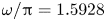 $\omega /{\rm \pi} =1.5928$) in an
  $x$-symmetric
  $y$-symmetric system; (c,d)
  $\textrm {Re}(\,p)$ of LMs (
 $L=1.4085$,
  $\omega /{\rm \pi} = 1.5096+ 1.324 \times 10^{-4} \mathrm {i}$;
  $L=1.9861$,
  $\omega /{\rm \pi} = 1.5942+ 1.346 \times 10^{-4} \mathrm {i}$) in an
  $x$-asymmetric
  $y$-symmetric system, where the heights of the left and right semi-infinite waveguides are
  $H_{left}=1$ and
  $H_{right}=1.1$. The LMs are calculated with the same
  $L$ as the TMs.
To have zero net transmission to  $k_2^+$ DM in the right semi-infinite waveguide, the incident waves in the cavity segment need to satisfy
 \begin{equation} \frac{C_2^+}{C_4^+} =- \frac{T_{24}}{T_{22}}, \end{equation}
where  $T_{22}$ and
  $T_{24}$ respectively denote the transmission from
  $k_2^+$ and
  $k_4^+$ DMs in the cavity segment to
  $k_2^+$ DM in the right semi-infinite waveguide. Then, each of the incident waves are totally reflected, as proved in § 4.4, thus
 \begin{equation}
\biggl| \frac{C_2^-}{C_4^-} \biggr| = \biggl| \frac{C_2^+}{C_4^+} \biggr|.
\end{equation}
\begin{equation}
\biggl| \frac{C_2^-}{C_4^-} \biggr| = \biggl| \frac{C_2^+}{C_4^+} \biggr|.
\end{equation}
If  $\Delta H >0$, then
 \begin{equation} \biggl|
\frac{T^-_{24}}{T^-_{22}} \biggr| \neq \biggl|
\frac{T_{24}}{T_{22}} \biggr|,
\end{equation}
\begin{equation} \biggl|
\frac{T^-_{24}}{T^-_{22}} \biggr| \neq \biggl|
\frac{T_{24}}{T_{22}} \biggr|,
\end{equation}
where  $T^-_{22}$ and
  $T^-_{24}$ respectively denote the transmission from
  $k_2^-$ and
  $k_4^-$ DMs in the cavity segment to
  $k_2^-$ DM in the left semi-infinite waveguide. Equations (5.2), (5.2) and (5.4) mean that the zero transmission to outgoing
  $k_2^{\pm }$ DMs respectively in the right and left semi-infinite waveguides cannot happen simultaneously when
  $\Delta H >0$. The zero transmission at both ends can happen in the
  $x$-symmetric system (figures 9 and 22a,b) and in the rotational symmetric system (figure 10), thanks to the same modulus of the transmission coefficient ratios on the left and right ends.
Note in figure 19 that eigenfrequencies vary continuously with  $L$, indicating that a slightly LM would occur if the system parameters depart slightly from the exact values for a TM. We also note that, in practice, there are no temporally non-decaying acoustic resonant modes because thermoviscous damping is always present and thus from the practical point of view it is meaningless to distinguish a very small
  $\mathrm {Im}(\omega _{LM})$ owing to radiation, e.g.
  $\mathrm {Im}(\omega _{LM}) \sim 10^{-4}$ in figure 21, from
  $\mathrm {Im}(\omega _{TM})=0$ corresponding to zero radiation. From the theoretical point of view, however, the difference between
  $\mathrm {Im}(\omega _{LM}) = 10^{-4}$ and
  $\mathrm {Im}(\omega _{TM})=0$ is significant (von Neumann & Wigner Reference von Neumann and Wigner1929a; Ursell Reference Ursell1951).
6. Conclusion
We investigate and compare various types of acoustic TMs in resonator–waveguide systems. The goal is to understand the commonality and difference between the mechanisms of common (symmetry protected, invisibility protected and symmetry– periodicity protected) and accidental TMs, which occur continuously and discretely in the resonator length–frequency ( $L$–
$L$– $\omega$) two-parameter space.
The key idea of this study is that all TMs can be explained by only examining the eigenfunctions of the TMs themselves, disregarding eigenvalue loci. Specifically, we define TMs by means of two conditions, i.e. the eigenmode and wave-trapping conditions, formulate them with the travelling-wave components of the eigenfunctions and then analyse why and how the propagating-wave loops in the eigenfunctions can satisfy the eigenmode (loop magnitude and phase constraints) and wave-trapping (loop zero-radiation) conditions simultaneously. To simplify the task, inspired by the asymptotic equation of the eigenmode condition and the visually simple eigenfunctions of long TMs, we analyse TMs with  $L \gg 1$. Therefore, the analysis is rigorous only in the asymptotic sense.
The analysis reveals the commonality of TM mechanisms studied, that is, one or multiple coupled propagating-wave loops (or submodes) in the resonant region satisfy TM conditions. For instance, the symmetry-protected TMs in the plate–waveguide system and the Friedrich–Wintgen TMs in the cavity–waveguide system, explained previously by totally different mechanisms, are actually the same in the sense that they are both underpinned by two coupled submodes. The commonality, found amidst long TMs in segmented-homogeneous resonator–waveguide systems, however, suggests that the unification of TM mechanisms and thus a unified explanation of all TMs can be pursued. The analysis also reveals the difference between common and accidental TMs, lying in how the loop zero-radiation condition is satisfied by propagating-wave loops. In common TMs, loop zero radiation is ensured alone by the particular amplitude ratio between the propagating-wave loops and it is independent of the single loop phase constraint that selects  $\omega _{TM}$ as a continuous function of
  $L$, due to the geometrical properties of the systems. On the other hand, loop zero radiation in accidental TMs depends on not only the amplitude ratio between the propagating-wave loops but also the loop phase constraints and there are two phase constraints. Only at the crossing points of the two phase constraints can zero-radiation loops be ensured, which is the reason for the discrete appearance of accidental TMs in the
  $L$–
$L$– $\omega$ two-parameter space.
In contrast to previous studies, the analysis suggests that phenomena such as modal degeneracy, avoided crossing and resonance-width bifurcation are not the mechanisms of accidental TMs. A counterexample that indicates the failure of avoided crossing and resonance-width bifurcation as predictive indicators for the occurrence of accidental TMs is provided.
Funding
This work has been supported by the National Natural Science Foundation of China no. 51876120.
Declaration of interests
The author reports no conflict of interest.
Appendix A. On the phase change in total reflection at waveguide discontinuities
The numerical results of the phase change in total reflection at waveguide discontinuities in § 4 show a common characteristic: the phase change is exactly  ${\rm \pi}$ at the lower limit of the frequency range of total reflection, whereas it is close to
  $0$ at the upper limit. Such a phase characteristic can be seen in the total reflection of a single DM (figure 13b) and of multiple DMs with the same phase change (figures 14b, 15b and 16b). It can also be observed from the latter cut-on DM in the total reflection of multiple DMs with different phase changes (figures 17b, 18b and 20b). Whether the discontinuity is a sudden constriction as in the cavity–waveguide systems or a sudden expansion as in the plate–waveguide systems for the incident DMs is not relevant to this phase characteristic.
The  ${\rm \pi}$-phase change at the lower limit of the frequency range can be rigorously explained. In figure 13(b), for example, the lower limit of frequency
  $\omega /{\rm \pi} =0.5$ is the cut-on frequency of
  $k_2^+$ wave in
  $d1$, i.e.
 \begin{equation} k_{2,{d1}}^+= 0. \end{equation}
The reciprocity relations of DM reflection and transmission at a waveguide discontinuity read (Cho Reference Cho1980)
 \begin{equation} k_{i,{d1}}^+ R_{ij} = k_{j,{d1}}^+ R_{ji}, \end{equation}
where  $k_{i,{d1}}^+$ and
  $k_{j,{d1}}^+$ denote the wavenumbers of
  $k_i^+$ and
  $k_j^+$ DMs in
  $d1$,
$d1$,  $R_{ij}$ is the reflection coefficient from
  $k_j^+$ to
  $k_i^-$ DM in
  $d1$ and
  $R_{ji}$ is reflection coefficient from
  $k_i^+$ to
  $k_j^-$ DM in
  $d1$
$d1$
 \begin{equation} k_{i,{d2}}^+ T_{ij} = k_{j,{d1}}^+ T_{ji}^-, \end{equation}
where  $k_{i,{d2}}^+$ denote the wavenumber of
  $k_i^+$ DM in
  $d2$,
$d2$,  $T_{ij}$ is the transmission coefficient from
  $k_j^+$ DM in
  $d1$ to
  $k_i^+$ DM in
  $d2$ and
  $T_{ji}^-$ is the transmission coefficient from
  $k_i^-$ DM in
  $d2$ to
  $k_j^-$ DM in
  $d1$. Combining (A1), (A2) and (A3) leads to
 \begin{equation} R_{i2}=0 \quad (i=1,3,4,\ldots) \end{equation}
and
 \begin{equation} T_{i2}=0 \quad (i=1,2,3,\ldots), \end{equation}
that is, the reflection to all the other cut-on and cut-off DMs (except  $k_2^-$ DM) in
  $d1$ and the transmission to all cut-on and cut-off DMs in
  $d2$, from the incident
  $k_2^+$ DM in
  $d1$ at its cut-on frequency, are zero. Thus, the pressure on the
  $d2$ side of the discontinuity is exactly zero. Pressure continuity requires that the pressure on the
  $d1$ side of the discontinuity must be also zero, which can only be satisfied by the
  ${\rm \pi}$-phase difference between
  $k_2^{\pm }$ DMs at the discontinuity. One can check that the continuity of acoustic velocity in the
  $x$- and
  $y$-directions across the discontinuity is satisfied. Some mode-to-mode reflection and transmission coefficients are plotted in figure 23(a,b), where zero reflection and transmission to other DMs (except
  $k_2^-$ DM in
  $d1$) from
  $k_2^+$ DM in
  $d1$ are shown at frequency
  $\omega /{\rm \pi} =0.5$. Figure 23(c) is very close to a pressure-release total reflection (
 $\kern0.7pt p = 0$ and
  ${\rm \pi}$-phase change), with
  $k_{2,{d1}}^+= 1.77 \times 10^{-5} \approx 0$ (the incident
  $k_2^+$ DM in
  $d1$ is just cut-on).

Figure 23. (a,b) Modulus of DM-to-DM reflection and transmission coefficients as  $k_2^+$ DM in
  $d1$ is incident on the waveguide constriction. Total reflection happens in the frequency range
  $0.5 \leq \omega /{\rm \pi} < 1$. The thick and thin lines, respectively, denote the corresponding reflected or transmitted DMs being cut-on and cut-off. (c) A nearly pressure-release total reflection of
  $k_2^+$ DM in
  $d1$ at frequency
  $\omega /{\rm \pi} =0.5+10^{-10}$ where
  $k_{2,{d1}}^+= 1.77 \times 10^{-5}$ (note the long wavelength of the incident
  $k_2^+$ DM in
  $d1$ of order
  $10^5$). (d) A nearly hard-wall total reflection of
  $k_2^+$ DM in
  $d1$ at frequency
  $\omega /{\rm \pi} =1\unicode{x2013} 10^{-10}$ where
  $k_{2,{d2}}^+= -2.51 \times 10^{-5} \mathrm {i}$ (note the hard-wall effect of the transmitted
  $k_2^+$ DM in
  $d2$).
Note that the exactly zero reflection and transmission to all the other DMs from a DM at its cut-on frequency also explain  $| C_1^+/C_2^+ | = 0$ in figures 17(a) and 18(a) and
  $| C_2^+/C_4^+ | = 0$ in figure 20(a) at the lower limit of the frequency ranges of total reflection.
The phase change being close to  $0$ at the upper limit of the frequency range, for example
  $\omega /{\rm \pi} =1$ in figure 13(b), is understood as the result of the hard-wall effect of the transmitted
  $k_2^+$ DM in
  $d2$ at its cut-on frequency where
  $k_{2,{d2}}^+=0$. Nevertheless, the mode-to-mode transmission coefficients to other DMs in
  $d2$ are small but not exactly zero at that frequency, as indicated by
  $|T_{42}| \neq 0$,
  $|T_{62}| \neq 0$ and
  $|T_{82}| \neq 0$ at
  $\omega /{\rm \pi} =1$ in figure 23(b). So, in general the phase change is close to but not equal to
  $0$ at the upper limit of the frequency range. Figure 23(d) is very close to a hard-wall total reflection (
 $\partial p / \partial x = 0$ and
  $0$-phase change), with
  $k_{2,{d2}}^+= -2.51 \times 10^{-5} \mathrm {i} \approx 0$ (the transmitted
  $k_2^+$ DM in
  $d2$ is still cut-off, but close to cut-on).


