


1. Introduction
As a large embayment on the northwest coast of Alaska, Kotzebue Sound (Fig. 1a) is a relatively sheltered environment in which to grow sea ice. Up until the early 21st century, sea ice would reliably fill the Sound each winter, creating a continuous expanse of landfast ice that spanned from shore to shore and bridged the ~50 km wide opening that connects it to the Chukchi Sea (Mahoney and others, Reference Mahoney, Eicken, Gaylord and Gens2014). Landfast ice that extends between shorelines like this is referred to as ‘landlocked’ (Hata and Tremblay, Reference Hata and Tremblay2015; Mahoney, Reference Mahoney2018) and Kotzebue Sound is perhaps the largest region in North America occupied by such ice outside of the Canadian Archipelago. The landlocked nature of wintertime Kotzebue Sound sea ice has historically allowed local residents to hunt marine mammals at the flaw lead in the Chukchi Sea (Lucier and VanStone, Reference Lucier and VanStone1991; Huntington and others, Reference Huntington, Quakenbush and Nelson2016) and travel to coastal communities outside the Sound without having to follow the shoreline. This type of use makes the sea ice of Kotzebue Sound more like that found in the channels and fjords of the Canadian Archipelago and Greenland (Gearheard and others, Reference Gearheard2013) than the sea ice on neighboring coastlines in the Chukchi Sea. However, for the last decade, although sea ice has typically filled Kotzebue Sound, it has failed to become landlocked, leaving only a relatively narrow fringe of landfast ice attached to the coast and a discontinuous ice pack of mobile floes in the center.

Fig. 1. (a) Kotzebue Sound, surrounding communities and inflowing rivers. Blue box in inset indicates extent of map coverage. Red box indicates coverage of map in adjacent panel. (b) Landsat 8 true-color image showing landfast ice near Kotzebue on 4 April 2019, with the locations of the two MBSs and other drill hole ice thickness measurements made in 2018 and 2019. The charted location of the channel is taken from NOAA electronic nautical chart 16161. Beyond the extent of this chart, the location is based on satellite imagery during spring melt. Isobaths are determined from the Alaska Regional Bathymetric Digital Elevation Model (Danielson and others, Reference Danielson, Johnson, Solomon and Perrie2008).
The Chukchi Sea has experienced significant losses of sea ice in recent years, with delayed onset of freeze-up and earlier retreat contributing to a near-complete absence of sea ice in September in recent years (Thoman and Walsh, Reference Thoman and Walsh2019). These changes have led to substantial increases in the duration of the open water season in the Chukchi coastal communities, according to the Historical Sea Ice Atlas for Alaska (Walsh and others, Reference Walsh, Fetterer, Scott Stewart and Chapman2016), which provides weekly sea-ice concentration dating back to 1953. Over this record, the open water season in Shishmaref has lengthened from ~110 days to ~160 days, while at Utqiaġvik the season has grown from ~30 days to over 100 days, with the majority of this change occurring since the 1990s (Rolph and others, Reference Rolph, Mahoney, Walsh and Loring2018). However, at Kotzebue there has been a pattern of substantial interannual variability in the duration of the open water season, but little net change since the 1950s, with a trend of ~3 days more open water per decade (Rolph and others, Reference Rolph, Mahoney, Walsh and Loring2018). This may suggest that large-scale sea-ice concentration datasets do not capture all significant changes affecting sea ice in embayments like Kotzebue Sound, but it also likely reflects that Kotzebue Sound is a markedly different sea-ice environment than the larger Chukchi Sea. Not only is the Sound shallower and more sheltered, but it is influenced by fresh water discharge from four major river systems (Fig. 1a). It is therefore likely that sea ice in Kotzebue Sound will respond differently to the forces driving sea-ice retreat in adjacent waters.
Here, we present results from what we believe is the first systematic program of sea-ice and snow measurements in Kotzebue Sound. As part of the Ikaaġvik Sikukun project (ice bridges, in Iñupiaq), these measurements were conceived and designed under the guidance of an Indigenous Elder Advisory Council comprised of co-authors J.G., C.H., R.J.S. and R.S. Sr. In partnership with this Council, and adopting a practice of knowledge co-production (e.g. Behe and Daniel, Reference Behe and Daniel2018), we established a series of over-arching research questions related to sea ice and its use by the residents of Kotzebue. These questions reflect the holistic concerns of local community members whose livelihoods and lifestyles are intimately linked with the sea ice of Kotzebue Sound. Each question is multifaceted and requires bringing together new data and knowledge from a variety of disciplines. Our analysis here addresses glaciological matters related to three of these questions:
I. What environmental factors control the length of the bearded seal hunting season in Kotzebue Sound?
II. What snow and ice surface properties promote ringed seal denning and pupping?
III. Why was there so little sea ice in Kotzebue Sound in 2018 (and 2019)?
The first two of these questions were identified during the early stages of the project development prior to any field observations. Question I was prompted by concerns regarding rapid changes during spring when the sea ice in Kotzebue Sound breaks up and bearded seals (Erignathus barbatus, known locally in Iñupiaq as ugruk) can be hunted by boat. Ugruk have been the primary marine resource for the Iñupiaq people living on the northern coast of Kotzebue Sound for thousands of years and hundreds are typically harvested each year (Whiting, Reference Whiting2006). Hauser and others (Reference Hauser2021, in press) note that the duration of the ugruk hunting season has decreased significantly in recent years, but the start is strongly correlated with the break-up of ice in the channel in front of Kotzebue (Fig. 1b). This breakup has to occur before hunters can launch boats from shore. Therefore, provided there are ugruk to be found beyond the mouth of the channel when it breaks up, earlier breakup will favor a longer hunting season.
Question II arose from observations by members of our Advisory Council that in recent years the landfast ice near Kotzebue contains fewer pressure ridges than in the past and, hence, fewer places where snow collects in deep drifts. Ringed seals (Phoca hispida, known locally in Iñupiaq as natchiq) rely on such drifts to create lairs in which to give birth, raise young and avoid predators (e.g. Smith and Hammill, Reference Smith and Hammill1981; Smith and Lydersen, Reference Smith and Lydersen1991). Although the observations and analysis presented here do not pertain specifically to snow drifts around ice ridges, we are able to identify and quantify conditions under which deep snow on relatively thin ice is likely to lead to surface flooding, which promotes conditions that are likely to be unfavorable for young ringed seal pups in lairs.
Question III was put forward after our first year of observations, in 2018, during which Kotzebue Sound remained almost devoid of sea ice, except for a narrow margin of landfast ice in the shallow waters around its edge. Hence, our program of sea-ice observations in Kotzebue Sound began in a year in which ice conditions were unlike any previously seen or heard of by local Elders. Kotzebue Sound was similarly devoid of ice the following year, so we have extended the third question to also include 2019.
In the analysis that follows, we adopt a combined observational and modeling approach to address the three questions raised by our Advisory Council. Using a 1-D thermodynamic ice growth model, we simulate the variation in ice thickness observed along the centerline and at the edge of the channel used to reach hunting grounds for ugruk. This allows us to better understand the role of ocean heat in melting the ice above the channel and address Question I. Using the same model, we also simulate surface flooding observed at the same two locations, allowing us to better understand the role of this process in both the thermodynamic growth of the ice beneath and the potential impact on ringed seal habitat (Question II). Additionally, by forcing our model with historical air temperature measurements, we provide a historical context for better understanding our two years of sea-ice observations and addressing Question III by evaluating the role that ocean heat may have played in the lack of ice in these two anomalous years. In addressing all three questions, we develop a baseline of the current ice regime in Kotzebue Sound and improve our understanding of ice growth processes in a changing Arctic.
2. Data and methods
2.1 Sea-ice mass-balance measurements
Here, the term ‘mass balance’ refers to the change in the thickness (i.e. mass) of the ice in response to the net balance of thermal energy entering or leaving the ice. To monitor changes in the thickness of sea ice over time, we established mass-balance stations (MBSs) on the landfast sea ice at two locations near Kotzebue (Fig. 1b and Table 1). One of these stations was deployed in the center of the channel that fronts the community of Kotzebue and was named the ‘Channel’ station. The other station was deployed at the edge of the channel in a small embayment northeast of Kotzebue and was named the ‘Bay’ station. The water below the Channel site was ~12 m deep, while at the Bay site it was just over 3 m in depth. At each MBS, ice thickness was measured using ‘hotwire’ gauges, consisting of a length of narrow-diameter stainless steel cable passing through the ice with a wooden handle at the top and a steel weight at the bottom. Below the steel weight, each cable was attached to a length of insulated large-diameter copper wire that passed back up through the ice making a single, conductive loop. When a 12 V battery is connected to the free ends of one of these loops, the stainless steel heats up and the wooden handle can be lifted until the steel weight makes contact with the bottom of the ice. Ice thickness was measured by reading the position of the handle against a graduated stake frozen into the ice and calibrated to the length of cable between the wooden handle and steel weight (Fig. 2).

Fig. 2. Schematic of hotwire gauge showing the connection of 12 V battery to ends of joined copper wire and stainless steel cable. Circular insets illustrate how the measurement of ice thickness and snow depth are made using graduations marked on the stake. Note that the stakes were marked in inches for the familiarity of our local observers (1″ = 2.54 cm). The inset inside the dashed box shows the layout of hotwire and snow stakes.
Table 1. Location and deployment/retrieval information for each MBS

Each MBS consisted of four hotwire gauges laid out at the corners of an 8 m square. Inside of this, we placed a 3-by-3 grid of snow stakes, spaced 2 m apart (see inset in Fig. 2). The snow stakes were marked with graduations that allowed snow depth to be read at a distance without having to disturb the snow surface within the MBS footprint. We also measured snow depth at the stake for each hotwire gauge, providing a total of 13 measurements of snow depth each time the site was visited. Additionally, a TinyTag PT1000 datalogger and temperature probe were placed at the snow-ice interface within 1 m of one of the hotwire gauges when each site was deployed. These sensors have a stated precision of ±0.01°C. Overall, this design is similar to that described by Mahoney and Gearheard (Reference Mahoney and Gearheard2008), except for the addition of the length of copper wire to each gauge, which allows it to work in fresh water and to be operated using a battery instead of a generator.
Each year, the two MBSs were deployed shortly after the ice became safe for travel by foot and snow mobile (Table 1). Thereafter, each station was visited on an approximately weekly basis by one of three local observers (co-authors A.V.W. and R.J.S.; and V. Schaeffer), who assisted with installation and received training on how to make and report measurements. For the familiarity of our local observers and other residents of Kotzebue, the stakes were graduated at half-inch (1.27 cm) intervals, providing an accuracy of ±0.64 cm for all our snow depth and ice thickness measurements.
In addition to the regular measurements made at each MBS by local observers throughout winter, near-daily measurements were recorded in the course of other related on-ice activities during late April and May in 2018. As part of these activities, ad hoc observations of ice thickness and snow depth elsewhere on the landfast ice near Kotzebue were taken toward the end of the growth season in both 2018 and 2019. These allowed us to assess spatial variability in the landfast ice cover at the time of expected maximum thickness and identify the presence of flooded snow and snow ice away from the two MBSs. The locations of these measurements are shown in Figure 1b.
2.2 Kotzebue air temperature data and freezing degree days
To provide a multidecadal context for winter conditions in Kotzebue prior to our two field seasons in 2018 and 2019, we obtained historical hourly dry bulb air temperature data from the Ralph Wien Memorial Airport at Kotzebue dating back to 1 January 1945. These data were obtained from the National Centers for Environmental Information (see acknowledgements for URL). These data allowed us to determine the annual dates of freeze and thaw onset and the accumulation of freezing degree days (FDDs) each winter. Following a similar approach to Mahoney and others (Reference Mahoney, Eicken, Gaylord and Shapiro2007), we defined the initial onset of freezing as the first day in each year that the daily mean air temperature, T daily, was below 0°C and the forward-looking 7-day mean air temperature was also below freezing. We also defined the onset of continuous freezing as the first day of the longest continuous period during which the 7-day mean air temperature remained below freezing. The initial onset and onset of continuous thawing were similarly defined using daily mean air temperatures above 0°C. The date of initial onset of freezing was used as the start date, d f0, for accumulating FDDs, which we calculated by finding the cumulative negative sum of T daily, for those days, i, when T daily is below freezing:

2.3 1D sea-ice growth model
To better understand the growth and melt processes observed at each MBS, we developed a model to simulate ice growth using observations of air temperature and snow depth, based on the 1-dimensional mass-balance equation for sea ice:

Here, Q is the net balance of the thermal energy fluxes entering and leaving the ice, ρ i is the density of sea ice, C i is the specific heat capacity of sea ice, T is the temperature of the ice, t is time, L i is the latent heat of fusion of sea ice, and H i is ice thickness. In essence, Eqn (2) states that if the net energy balance is negative then the ice will become colder and thicker.
To simplify the energy balance, we neglect the energy flux required to change the temperature of the ice, since over the course of a season, this is at least an order of magnitude smaller than the heat flux required to grow or melt the ice cover based on a typical heat capacity and latent heat of fusion for sea ice of 4 kJ kg−1 K−1 and 330 kJ kg−1, respectively. We also assume that the radiative and turbulent heat fluxes combine such that the upper surface of the snow (or ice, if no snow is present) is at the same temperature as the atmosphere directly above it. We note that this may often not be the case when there is a rapid change in air temperature and a delayed response in surface temperature. However, over the course of the winter, we expect the net effect of these deviations to be small. The temperatures of the air and snow or ice surface will also differ any time the air temperature is above freezing, since the snow or ice will be constrained to the freezing point. During each year, thawing air temperatures occurred for a total duration of <12 days, with <4 days of air temperatures above 2°C. The net effect of any inaccuracy in surface temperature during these thawing events is therefore also considered to be small.
Following Maykut (Reference Maykut and Untersteiner1986), this allows us to express the energy balance as the sum of the conductive flux through the ice and snow, F c, and the vertical heat flux from the ocean into the bottom of the ice cover, F w:

The conductive flux depends on the effective thermal conductivity of the combined ice and snow cover, k eff, and the vertical temperature gradient between the ocean and atmosphere:

Assuming linear temperature gradients through the ice and snow (Maykut, Reference Maykut and Untersteiner1986), we can write:


where T f is the freezing point of the ocean, T air is the surface air temperature, H s is snow depth, and k i and k s are the thermal conductivities of sea ice and snow, respectively.
By assuming linear temperature gradients, then we can estimate the temperature at the snow-to-ice interface at the base of the snow pack, T si, if we also assume continuity of flux across this boundary:

Re-arranging equations (2–6) and expressing the temporal derivative as a finite difference gives us the following expression for the change in ice growth, ΔH i, over a short time interval, Δt:

Equation (8) allows us to simulate ice growth over time given an initial ice thickness and time series of air temperature, snow depth and ocean heat flux. To maintain a finite temperature gradient and realistic early growth rates, the initial ice thickness must be non-zero and should be significantly greater than the amount of ice that can be grown during a single time interval. In the results presented below, we specified an initial thickness of at least 0.1 m and used a time step of 1 hour. These parameters and other physical constants used in the model are listed in Table 2. We note that this simple model is not expected to perform well after the onset of melt, since radiative forcing becomes more important as insolation increases and the surface albedo decreases and the surface temperature cannot be assumed to be at the same temperature as the air.
Table 2. Parameters and values used in ice growth model and isostatic calculations

2.4 Surface flooding and snow ice formation
The effect of snow on the growth of sea ice is twofold. First, the snow acts as an insulator reducing the conductive flux and thereby leading to slower ice growth. However, snow also acts as a weight on top of the ice reducing its freeboard above the waterline. If enough snow accumulates, it can push the ice surface below sea level, allowing the base of the snow pack to flood (e.g. Maksym and Jeffries, Reference Maksym and Jeffries2000). Applying Archimedes' principle, the buoyancy force counteracting the weight of sea ice and snow is equal to the weight of seawater displaced. For unflooded snow, this can be expressed as:

where ρ s and ρ w are the density of snow and seawater, respectively, g is the acceleration due to gravity, and ${\cal F}$ is the freeboard of the ice surface. The difference $( {H_{\rm i}-{\cal F}} )$
 is known as the ice draft, or the distance of the ice bottom below the waterline.
Rearranging Eqn (9), we get an expression for the freeboard of snow-covered sea ice, which is the basis for altimetry-derived estimates of sea-ice thickness (e.g. Zwally and others, Reference Zwally, Yi, Kwok and Zhao2008):

Equation (10) holds for negative freeboard provided the snow remains dry as the ice surface is depressed below waterline. As Maksym and Jeffries (Reference Maksym and Jeffries2000) note, negative freeboard does not always lead to flooding and the surface may remain dry under several centimeters of negative freeboard if the ice beneath is sufficiently impermeable. However, if there is a pathway for seawater to reach the surface of the ice, then the snow will become wetted to a depth up to the magnitude of F. If this occurs, then the flooded snow displaces only a fraction of its volume, reducing the upward buoyancy force. To account for this, we subtract the weight of the water within the flooded snow pack from the right-hand side of Eqn (10). This leads to the following equation for the freeboard of sea ice with a flooded snow cover:

where v l is the volume fraction of the flooded snow occupied by liquid water and d f is the fractional depth of the negative freeboard that floods. Fritsen and others (Reference Fritsen, Coale, Neenan, Gibson and Garrison2001) estimated v l to be as high as 65% in flooded snow on Antarctic sea ice. In this case, if seawater has an efficient pathway to the ice surface (i.e. d f ≈ 1), then the magnitude of the negative freeboard could be more than twice what would be estimated using Eqn (10).
In our ice growth model, we calculate the freeboard at each time step to determine if it is negative and if so, we assume flooding occurs instantaneously. When making this calculation, we assume that early springtime thinning of the snow pack does not result in a loss of mass from on top of the ice, i.e. the thinning is either due to compaction or any meltwater remains within the snow. This assumption is consistent with Warren and others (Reference Warren1999) observation that snow density is greatest for ‘residual melting snow in July’. To achieve this, we keep track of cumulative snow mass, which counts only positive changes in snow depth. Once the base of the snow is flooded, the upper surface of the ice below is constrained to the freezing point. The temperature gradient through the ice is thereby reduced to zero and no further growth can occur at the bottom of the ice until the flooded snow refreezes. We treat this in our ice growth model by applying the mass-balance Eqn (2) at the top of any unfrozen flooded snow. The temperature gradient therefore becomes:

where $H_{{\rm s}_{{\rm dry}}}$ is the depth of dry snow and H si is the thickness of any refrozen snow ice. Hence, by assuming that the properties of refrozen snow ice are the same as sea ice and that only the liquid fraction of the flooded snow, v f, has to freeze, we get the following expression for the growth of snow ice:

where $H_{{\rm s}_{{\rm dry}}} = H_{\rm s} + {\cal F}$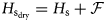 (for ${\cal F} < 0$
 ). The vertical ocean heat flux, F w, is still applied at the base of the ice, such that bottom melt can occur while the flooded snow is freezing into snow ice.
We recognize that the approach described here accounts only for the heat flux involved in the formation of snow and neglects the flux of salt associated with the flooding of the snow pack and subsequent freezing. Instead, by assuming that the resulting snow ice has the same properties as the underlying sea ice, we are in effect assuming that the brine in the flooded snow has the same composition as the seawater underneath the ice. This effectively assumes that the floodwater does not percolate through ice, in which case it would flush concentrated brine from within (Maksym and Jeffries, Reference Maksym and Jeffries2000). We also do not account for the concentration of the remaining brine in the flooded snow as it freezes, which will depress the freezing point in the slush leading to a reduction in the temperature gradient through the snow and snow ice and an increase in the gradient through the sea ice. We may therefore overestimate the rate at which any flooded snow freezes and slightly underestimate bottom growth. Thus, the effect on total ice growth is likely to be negligible, but we may underestimate the ocean heat flux, which is determined from the difference between the modeled and observed position of the ice bottom. Also, unlike Maksym and Jeffries (Reference Maksym and Jeffries2000), we do not consider convective heat flow in the brine volume.
2.5 Derivation of ocean heat flux as residual
Although we do not present any measurements from the water beneath the sea ice, we can estimate the vertical ocean heat flux, F w, using a ‘residual’ method (e.g. Krishfield and Perovich, Reference Krishfield and Perovich2005; Kirillov and others, Reference Kirillov, Dmitrenko, Babb, Rysgaard and Barber2015). This involves running the model without any ocean heat flux (F w = 0) and calculating the difference between modeled ice thickness, $H_{{\rm i}_{{\rm mod}}}$ , and observed ice thickness, $H_{{\rm i}_{{\rm obs}}}$
 . For each time step, it is then possible to determine the heat flux needed to explain the difference:

If the modeled ice thickness is greater than that observed, then F w will be positive, indicating an upward flux of heat into the ice, retarding ice growth or promoting melt. A negative value of F w would imply the ocean is acting as a heat sink. In the absence of deep ice shelves capable of supporting conditions for significant super-cooling of the ocean (e.g. Lewis and Perkin, Reference Lewis and Perkin1986), we consider any such results non-physical. In calculating F w using this method, we apply a two-step smoothing process to reduce sensitivity to small variations when calculating multiple differences. We first apply a 7-day smoothing filter to the difference between modeled and observed thicknesses and then apply a 30-day smoothing filter to the temporal derivative of this value. This approach partly helps account for the fact that we neglect heat storage in the ice and snow, which would otherwise reduce short-term variability in the model.
3. Results
3.1 Anomalously warm winters at Kotzebue in 2018 and 2019
The August-to-July mean temperatures in 2017–18 and 2018–19 were the warmest such 12-month periods in the 74-year record from 1945 to 2019, at −1.22 and 0.37°C, respectively. Although no daily air temperature records were set during either 12-month period, most days during both annual cycles were warmer than the full-record mean (Fig. 3a). Between August 2017 and July 2018, there were 56 days when the daily mean air temperature was among the warmest 10% for that calendar day. During the same period in 2018–19 there were 156 such days. It should be noted that unusually cold days also occurred in both years, but they were much rarer than warm days with just 6 days among the coldest 10% in 2017–18 and two such days in 2018–19.
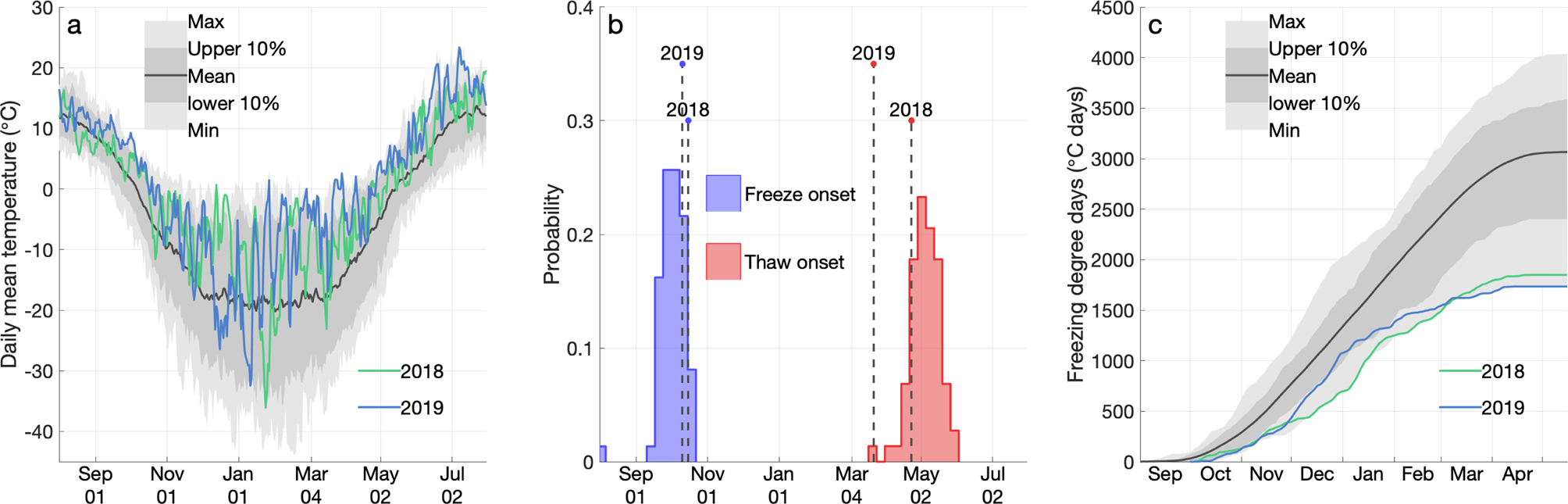
Fig. 3. (a) Annual cycle of air temperature measured at Kotzebue airport from 1 August to 31 July in 2018 and 2019, overlaid on the climatological mean and range from 1945 to 2019. (b) The distributions of initial freeze and thaw dates, as defined in section 2.2, over the duration of the record, with the dates for 2018 and 2019 shown. (c) Accumulation of FDDs during the 2017–18 and 2018–19 winters, overlaid on the climatological mean and range from 1945–2019.
In 2017 and 2018, the initial onset of freezing temperatures (section 2.2) occurred on 15 October and 10 October, respectively. These are both later freeze onsets than the 74-year mean date of 1 October, but they are not the latest in the record (Fig. 3b). In 2018 and 2019, the initial onset of thawing temperatures occurred on 22 April and 21 March, respectively, with the latter being the earliest onset of thaw on record at Kotzebue. Between the initial freeze and thaw onset dates, the freezing season in 2018–19 was the shortest in the 74-year record at 163 days. In 2017–18, the freezing season lasted 190 days, which was the fourth shortest in the record. However, the anomalous warmth during the winters of 2017–18 and 2018–19 at Kotzebue is illustrated most clearly by the record of FDDs accumulated over time (Fig. 3c). These two winters represent the two lowest end-of-winter FDD totals on record. Furthermore, on most days of the year, the lowest partial-season FDD accumulation occurred in either 2017–18 or 2018–19.
3.2 Observed snow depth and ice thickness in 2018 and 2019
MBS data from both the Channel and Bay stations show that landfast sea ice near Kotzebue was significantly thinner in 2019 than 2018 and had a deeper snow cover (Fig. 4). At the Channel MBS, the ice reached a maximum mean thickness of 0.86 m in 2018, compared with 0.50 m in 2019. At the Bay MBS, the maximum mean ice thickness was 1.00 m in 2018 and 0.64 m in 2019. Hence, at both stations, the sea ice was over 35% thinner in 2019 than in 2018. The difference in ice thickness between the two years is at least partly explained by the difference in snow depth. In 2018, the peak mean snow depth at the Channel and Bay MBSs was 0.25 and 0.42 m, respectively. In comparison, the corresponding peak mean snow depths in 2019 were 0.29 and 0.62 m, or ~50 and 16% thicker, respectively. However, although the deeper snow cover in 2019 than 2018 was associated with thinner sea ice beneath, this relationship does not hold when comparing observations between the two stations. In both 2018 and 2019, the ice at the Bay MBS was thicker than at the Channel MBS, despite also having a deeper snow pack. In both 2018 and 2019, drill hole measurements made elsewhere in the landfast ice (Fig. 1b) indicated that ice thickness in the shallow water away from the channel was somewhat thicker than that measured at the MBS, typically between 0.8 and 1.2 m. Since the drill hole measurements in 2019 were not made at the same locations as those in 2018, we cannot evaluate interannual differences from these data.

Fig. 4. Snow depth, sea-ice thickness and snow ice thickness measured at the Channel and Bay MBS in 2018 and 2019. Solid lines indicate mean values from all stakes, while dashed lines indicate the range of minimum and maximum values. To avoid clutter, the minimum and maximum snow ice thicknesses are not shown, but the range was similar to that for snow depth. The tick marks on the horizontal axes indicate the timing of MBS observations. Some tick labels are omitted where observations are closely spaced in time. Note that snow ice observations are more sparse than other observations and are therefore specifically indicated by black triangles.
Another notable difference between our two years of observations was the prevalence of snow ice formation (see section 2.4) in 2019. The MBS design does not provide a direct means to observe the composition of snow beneath the surface, but by careful probing of the snow during some visits to the MBSs, we were able to identify the top of any frozen slush at the hotwire stakes without otherwise disturbing the snow pack. The extent of snow ice was observed in more detail during the extraction of each MBS. In Figure 4, we interpolate between these sparse observations of the snow ice surface, and for illustration purposes, we do not attempt to distinguish between snow ice and unfrozen slush. Drill holes made elsewhere in the landfast ice in April (Fig. 1b) found that surface flooding was not just restricted to the MBS locations. Snow ice layers between 0.33 and 0.38 m thick were observed in ice cores extracted at multiple drilling locations in 2018. However, the freeboard in these core holes was typically zero or only slightly negative, indicating that the occurrence of flooding is likely to be under-observed if sufficient time elapses for the wet snow to refreeze and the position of the original ice surface is not recorded. The 0.38 m thick layer was observed adjacent to a flooded seal lair (see Fig. 1b for location), where the original ice surface was submerged below 0.38 m of water.
In 2018, we first observed snow ice formation on 28 April and 5 May at the Channel and Bay MBS, respectively, but data from the TinyTag temperature sensors suggest initial flooding may have occurred on 24 April and 10 April (see section 3.3). When the stations were recovered in 2018, we measured an average snow ice thickness above the initial ice surface of 0.03 m at the Channel station and 0.14 m at the Bay station with no unfrozen slush layer present. In 2019, we made only one snow ice observation at the Channel site prior to the end of the season, but based on the premature end of the TinyTag temperature record (section 3.3), we infer that the ice surface flooded and snow ice started forming at the Channel MBS on 14 February and at the Bay MBS on 12 February. During recovery in 2019, there was an average of 0.20 m of snow ice that had formed above the original ice surface at the Channel MBS with little unfrozen slush remaining. Of particular note, we found that the underlying sea ice had completely disappeared due to bottom melt at one hot wire gauge at the Channel MBS, leaving only snow ice that formed since deployment. Since the hotwire gauges do not directly account for snow ice development, this led to a disconcerting measurement of ‘negative’ ice thickness. When the Bay MBS was recovered in 2019, the top of the snow ice layer was an average of 0.44 m above the original ice surface, with a greater amount of unfrozen slush beneath. There was no clear interface between the slush and the snow ice, making it difficult to measure the thickness of the frozen snow ice layer.
Another remarkable feature of the MBS data is that the bottom growth of landfast ice near Kotzebue ceased by mid-February at the Channel MBS in both 2018 and 2019 and at the Bay MBS in 2019. In 2018, sea ice at the Bay MBS continued thickening through bottom growth until mid-April, approximately coinciding with the onset of thawing air temperatures (Fig. 3b). However, in all other cases, bottom growth ceased several weeks before thawing occurred at the surface. The role of snow ice formation and vertical ocean heat flux in the cessation of bottom growth is discussed further below (section 4.1). Lastly, we note some peculiar variability in ice thickness measured by the hotwire gauges at both MBSs in early May in 2018. For reasons we do not fully understand, multiple hotwire gauges showed abrupt losses of up to 15 cm of ice, which was followed by an increase of similar magnitude within the next 1–3 days. Different gauges showed this behavior on different days. Had the loss of ice persisted, this may have indicated that the weight had somehow slipped on the stainless cable. Alternatively, if we had observed an abrupt but short-lived increase in thickness, we could have interpreted this as the formation of a false bottom due to the interaction of fresh meltwater with saline seawater at its freezing point (e.g. Notz and others, Reference Notz2003). However since neither of these explanations fits the observations, we instead put forward the tentative explanation that the bottom of the ice was becoming highly uneven at this time and that on some occasions, the weight would be pulled up into a small cavity on the underside of the ice. Under-ice video footage collected in April 2019 revealed a highly scalloped bottom, supporting this possibility.
3.3 Temperature at the bottom of the snow-pack
The snow-ice interface temperatures recorded by the TinyTag sensors at each site provide a means for deriving an appropriate value for snow thermal conductivity, k s, for our 1-D growth model (section 2.3). We forced the model with hourly airport air temperature observations (section 3.1) and snow depth measurements from the MBS (section 3.2), which were linearly interpolated to an hourly time interval. We ran the model for each year and MBS location with three different values of k s and compared the derived values of T si (Eqn (7)) with observations from the TinyTag temperature sensors (Fig. 5). For this comparison, we have excluded observations associated with flooding of the snow pack, as described below. Even so, the agreement is not perfect since we do not account for thermal lag in the snow pack, which smooths out short-term variations, particularly as the snow gets deeper. However, for both years and both MBS locations, we found a value of k s = 0.3 resulted in the lowest rms difference between modeled and observed T si for most cases (Table 3).

Fig. 5. Comparison between observed and modeled snow-ice interface temperature, T si, using different values of snow thermal conductivity, k s.
Table 3. Root-mean-square (rms) difference between observed and modeled values of T si for three values of k s

During January and early February in both 2018 and 2019, the temperature at the bottom of the snow pack, T si, remained strongly coupled to air temperature (Fig. 6). In 2018, T si became more stable as the snow pack deepened and despite air temperatures below −20°C in February and March, T si remained in the range −6 to −3°C until abrupt warming events on 10 April at the Bay MBS and 24 April at the Channel MBS. These warming events resulted in step changes in T si, which remained close to 0°C for the remainder of the record. We therefore interpret these events as the onset of flooding at the base of the snow pack. In 2019, the TinyTag temperature sensors at both MBSs started recording spurious values on 12 and 14 February, at the Bay and Channel MBS, respectively. We presume this was caused by surface floodwater penetrating the sensors, which sustained minor damage when they were extracted from refrozen snow ice in 2018 that may have compromised any water resistance.

Fig. 6. Observed air temperature, T a (grey) and bottom-of-snow temperature, T si (black), compared with modeled T si for snow thermal conductivity, k si = 0.3 W m−1 K−1 at each MBS deployment. Due to flooding-related damage to TinyTag sensors, the observed T si record in 2019 was cut short.
3.4 Simulated sea-ice growth in 2018 and 2019
Each time step, the 1D growth model calculates the isostatic freeboard based on ice thickness, snow depth and the depth of any flooding. When calculating negative freeboard, we assume d f = 1, implying that there are efficient pathways for seawater to reach the ice surface, and v l = 0.65, implying the air volume in the snow was almost completely filled with water. In both 2018 and 2019, the total amount of modeled flooding at the end of the season agrees well with the observed amount of snow ice at both MBSs when they were extracted (Fig. 7). This indicates the isostatic calculations in our growth model are accurate. In 2018, the 1D model predicts flooding over a month before any snow ice was observed, suggesting that flooding did not occur instantly when the freeboard became negative. In 2019, there is excellent agreement between the isostatically predicted onset of flooding at the Channel MBS (Fig. 7c) and the inferred start of flooding based on the start of spurious measurements from the TinyTag temperature sensor (section 3.3, Fig. 6b). At the Bay MBS, the model predicts a few centimeters of flooding at the beginning of the record, which was not observed during deployment, followed by a rapid increase in flooding in mid-February (Fig. 7d), approximately coinciding with the end of the TinyTag temperature record (Fig. 6d).
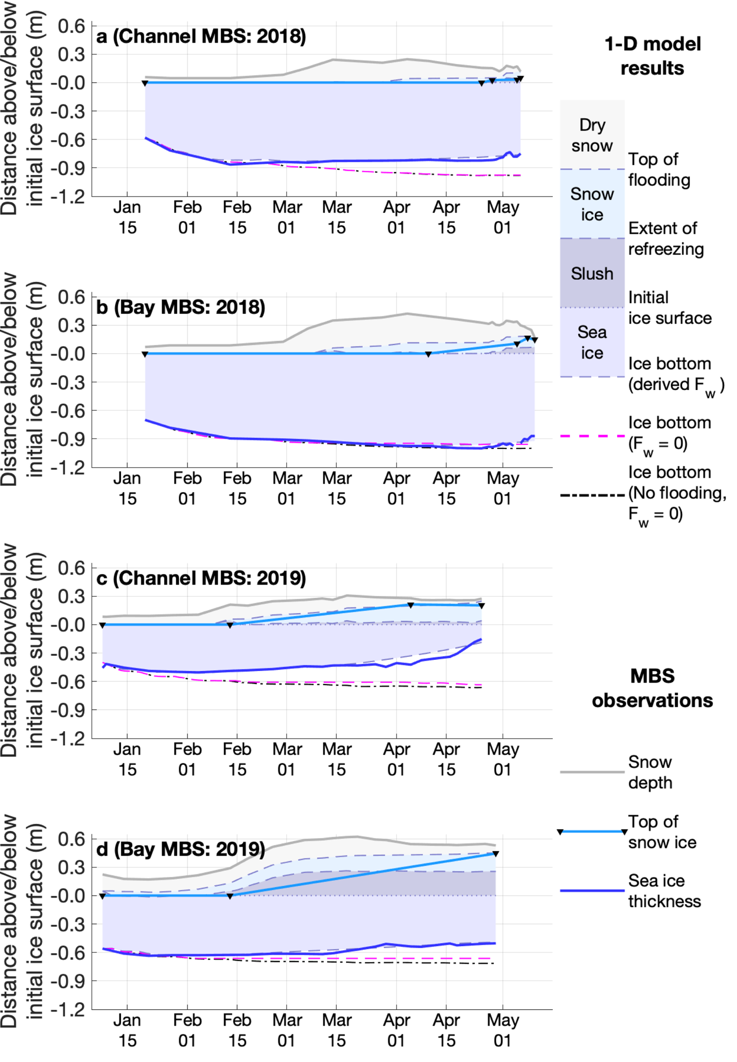
Fig. 7. Modeled ice growth, depth of dry snow, depth of flooding and snow ice formation (shaded polygons and dashed lines) compared with MBS observations (solid lines). Observations of the top of snow ice are more sparse than other observations are marked with black triangles.
In addition to accurately predicting the depth of flooding of the snow pack, our model appears to qualitatively reproduce the observed amount of snow ice formation. The model predicts complete or near-complete freezing of the flooded snow layer at both MBSs in 2018 and at the Channel MBS in 2019 (Fig. 7), in agreement with observations. At the Bay MBS in 2019, our model indicates that only approximately half of the 0.44 m of flooded snow refroze, which is consistent with the observations of unfrozen layers or cavities within the snow ice during extraction of this station.
If we do not account for snow ice formation and we assume that the vertical oceanic heat flux, F w, is zero, then our model significantly overestimates the growth that occurs at the ice bottom compared with MBS hotwire measurements (dashed black lines and solid blue lines, respectively, in Fig 7) in all cases except the Bay MBS in 2018. Initially, we suspected that the formation of snow ice at the upper surface of the sea ice could account for this difference. However, when we account for the latent heat required to freeze flooded snow at the upper ice surface (dashed magenta lines in Fig. 7), we find that the resulting difference in bottom position is considerably smaller than the thickness of snow ice formed and accounts for only a small fraction of the difference between the modeled and observed ice bottom position. If we instead assume the difference in ice growth is primarily due to a non-zero ocean heat flux, then we can use the approach described in section 2.5 to derive an estimate of the variation in F w at each MBS over each season (Fig. 8).

Fig. 8. Vertical ocean heat flux, F w, derived from the difference between hotwire MBS observations and modeled ice bottom position accounting for snow ice formation (see Fig. 7).
The results of this approach indicate that F w is consistently higher in the center of the channel (red lines in Fig. 8) than at its edge (blue lines) and that F w was significantly greater in 2018 than 2019. There is also a tendency for F w to increase over the course of each winter, particularly toward the end of the season. However, due to heavy smoothing carried out in the derivation of F w, we avoid the discussion of variability at shorter timescales. The modeled ice bottom positions using F w derived through this approach are shown by the dashed lines at the base of the sea-ice polygons in Figure 7. The good agreement with the observed ice bottom position demonstrates that our approach captures the majority of the variability in F w between locations and over time. We note that Figure 8a indicates a period of apparent negative ocean heat flux at the Bay MBS in late February and March 2018. As discussed in section 2.5, this is treated as a non-physical result and is possibly caused by an underestimate of the thermal conductivity of snow or sea ice, resulting in an underestimate of the conductive flux, F c. At its most negative, F w reaches −3 W m−2, which is within the accuracy with which we can expect to resolve the ocean heat flux using this method (see section 4.1).
4. Discussion
4.1 Role of ocean heat flux in break-up of sea ice in the channel
As discussed in section 1, the break-up of sea ice in the channel in front of Kotzebue is a controlling factor determining when bearded seal hunting can begin. Hence, understanding the role of ocean heat flux in this break-up helps us address research question I: What environmental factors control the length of the bearded seal hunting season in Kotzebue Sound? Although a comprehensive assessment of the factors controlling this annual break-up is beyond the scope of this paper. However, thinning and weakening of the ice in the channel is one necessary step before it can be dislodged and flushed into Kotzebue Sound beyond the landfast ice by the down-channel current. Our results shed light on the thermodynamic processes that control the thickness of ice in the channel and the rate at which it thins prior to break-up.
In 2018, the modeled rate of ice growth without ocean heat flux is initially in agreement with observations at both MBSs. However, the early cessation of ice growth at the Channel MBS and achievement of a near-equilibrium ice thickness of ~0.80 m (Fig. 7a) indicates that F w soon began increasing and reached a value of ~10 W m−2 by mid-March (Fig. 8a). By comparison, the ice at the Bay MBS continued growing at a rate consistent with no ocean heat flux until late April (Fig. 7b) at which point our model suggests F w likely reached a similar value to that at the Channel MBS. In 2019, there appears to have been a significant ocean heat flux when our measurements began. The slow rates of growth observed at both MBS despite low air temperatures, relatively thin ice and shallow snow indicate that F w was already ~10 W m−2 in early January at the Channel MBS and 5 W m−2 at the Bay MBS. Interestingly, our results indicate opposite trends in F w at the two MBSs toward the end of the season. The rapid bottom thinning observed at the Channel MBS in April 2019 (Fig. 7c) suggests F w reached values as high as 30 W m−2 before the station was recovered (Fig. 8b), whereas the last 2 weeks of measurements at the Bay MBS show an apparent pause in bottom melt (Fig. 7d) indicating a reduction in F w. This asynchronous variability suggests that there was likely along-channel variability in F w as well as cross-channel variability.
It is clear from our observations and modeling results that the vertical flux of heat from the ocean into the bottom of the ice played a significant role in the mass balance and resulting thickness of sea ice at both MBS locations in both 2018 and 2019. The source of this heat is the subject of ongoing research analyzing data from oceanographic moorings deployed in Kotzebue Sound during the same period (Witte and others, Reference Witte2021). Our results here show that F w was greater at the Channel MBS than at the Bay MBS, which is consistent with the expectation of stronger currents in the center of the channel, resulting in a greater transfer of heat to the ice through turbulent processes (McPhee, Reference McPhee1992). Our results also show that F w at the Channel MBS was significantly greater in 2019 than it was in 2018 (Fig. 8), which not only led to an ice cover that was substantially thinner in 2019 than 2018 (Figs 4 and 7), but also is consistent with the earlier start to the ugruk hunting season in 2019 (Hauser and others, Reference Hauser2021, in press). This suggests that monitoring of ice thickness and vertical heat flux in the channel through the winter would likely be useful for predicting the timing of channel break-up.
By deriving the vertical flux of ocean heat as that required to compensate for the difference in the position of the ice bottom measured by the hotwire gauges and the modeled ice bottom with F w = 0, we are effectively assuming that our model successfully captures all other significant fluxes that affect the mass balance of landfast sea ice near Kotzebue. We acknowledge that it could instead be possible that our model overestimates the conductive flux of heat through the ice or neglects another source of heat, both of which would lead to excessive ice growth compared to observations.
For reference, at the beginning of the record when air temperature is lowest, the snow and ice are thinnest and the conductive flux is hence greatest, a difference of 0.1 W m−1 K−1 in the value of k s equates to a difference of ~5 W m−2 in the derived value of F w. However, as discussed in section 3.3, we selected a value of k s = 0.3 W m−1 K−1, since this resulted in a smaller rms difference between observed and modeled values of T si than either k s = 0.2 or 0.4 W m−1 K−1 (Fig. 5 and Table 3). Moreover, this sensitivity reduces over time as the conductive flux decreases. Additionally, if we are underestimating the k s, then derived values of F w for conductive flux at the Bay MBS in 2018 (Fig. 8a) would be even more negative. We therefore conservatively expect our estimate of F w to have an uncertainty of <5 W m−2.
It is clear from the hotwire measurements that the thinning is taking place at the bottom of the ice and therefore any residual heat flux must be acting at the ice-ocean interface. Hence, we are confident that vertical ocean heat flux accounts for the majority of the difference between our MBS observations and the modeled ice thicknesses. The magnitudes of F w we calculate in 2018 are similar to those derived from similar measurements in coastal settings in Greenland (Mahoney and others, Reference Mahoney, Gearheard, Oshima and Qillaq2009; Kirillov and others, Reference Kirillov, Dmitrenko, Babb, Rysgaard and Barber2015), while in 2019 our highest measurements are comparable to those reported for summertime in the Central Arctic based on similar ‘residual’ methods and turbulent heat flux measurements (Krishfield and Perovich, Reference Krishfield and Perovich2005).
4.2 Importance of surface flooding and snow ice formation
Snow ice formation was observed at both MBSs in both years. In 2018, it accounted for ~4 and 14% of the final average thickness at the Channel and Bay MBS, respectively (Figs 4a, b), while in 2019 it amounted to approximately half the total thickness at both MBSs (Figs 4c, d). At one hotwire gauge at the Channel MBS, snow ice accounted for 100% of the remaining thickness after bottom melt removed the original underlying ice. Surface flooding and subsequent snow ice formation therefore played a significant role in the mass balance of landfast sea ice near Kotzebue in 2019. Although bottom growth slows or ceases while the flooded snow is freezing, the additional thickness of snow ice at the upper ice surface resulted in only a small reduction in bottom ice growth. This means that had the snow remained unflooded, the ice in the channel would have been significantly thinner and therefore would likely have broken out even earlier.
Overall, the impact of snow cover on ice growth is negative due to its insulating effect. Although the formation of snow ice makes a positive contribution, this does not offset the insulating effect of the snow required to cause the flooding. At the end of the 2019 Channel MBS record, our model indicates that there was 0.21 m of sea ice with 0.20 m of flooded snow on top, of which 0.19 m had frozen to form snow ice. This is in good agreement with the MBS observations and amounts to a total ice thickness of 0.41 m. By comparison, if we run the growth model with zero snow and keep all other parameters the same, we find a total ice thickness of 0.61 m. We can extend this comparison by simulating ice growth at both MBSs under different snow depth scenarios, which we create by multiplying the observed snow depths by a ‘snow depth factor’ between 0 and 2. The results of this model experiment indicate there is a local minimum or an inflection point in total thickness corresponding to the snow depth factor that results in a freeboard of zero and the onset of snow ice formation (Fig. 9). In 2018, this suggests there may have been a slight decrease in total thickness for a modest reduction in snow depth. However, overall there is a negative relationship between total ice thickness and snow depth.

Fig. 9. Modeled total sea-ice thickness and the contribution from snow ice on 1 April at each MBS in 2018 and 2019 under varying snow depth. A snow depth factor <1 indicates less snow than observed, while a factor >1 indicates more snow. Total thickness represents the thickness of both sea ice and snow ice.
The observed depth of flooding indicates that no dry snow remained below the waterline, which corresponds to our assumed value of d f = 1 and suggests the floodwater had an efficient pathway to the top of the ice, though either holes, cracks or the permeability of the ice beneath. Moreover, the accuracy with which the model reproduces the observed levels of flooding at both MBSs in both years validates our isostatic calculation, which accounts for the volume of water in the flooded snow (Eqn (11)). This does not appear to be a widespread practice in previous studies of flooded snow, but had we neglected the reduced buoyancy of wetted snow, we would have underestimated the depth of flooding observed at the MBSs by at least half. We are aware of only one other study that has taken this approach (Kirillov and others, Reference Kirillov, Dmitrenko, Babb, Rysgaard and Barber2015) and our results are in agreement with theirs.
Surface flooding was not initially considered when we conceived research question II, which asked What snow and ice surface properties promote ringed seal denning and pupping? Nonetheless, such flooding is likely to impact ringed seals, who excavate lairs in the snow on top of sea ice to provide refuge from predators throughout winter and for birthing and raising young in spring (e.g. Smith and Stirling, Reference Smith and Stirling1975; Smith and Hammill, Reference Smith and Hammill1981; Smith and Lydersen, Reference Smith and Lydersen1991). No ringed seal lairs were observed in the vicinity of either MBS, but during other field observations near Sisualik (see Fig. 1b), we found a lair in late April 2018 that appeared to have flooded to a depth of over 0.38 m during the winter. An ice core extracted adjacent to the seal lair revealed 0.38 m of refrozen snow ice with 0.46 m of sea ice below, showing that the flooding was not limited to the seal hole. Equation (11) predicts that 0.26 m of dry snow above the wet snow would be required to cause this amount of flooding. At the time of observation, there was an average of 0.31 m of dry snow, indicating that the flooding was likely caused by snow loading.
Birth lairs are particularly important for ringed seal pups that are born with a white fur coat called lanugo to provide insulation for ~2–3 weeks until sufficient fat reserves accumulate. However, lanugo cannot retain its insulation when wet, such that wetted pups become hypothermic if they cannot dry or are unsheltered (Smith and others, Reference Smith and Lydersen1991). No members of our Advisory Council recall previously observing flooded ringed seal lairs and there are few references to this phenomenon in scientific literature. Kelly and others (Reference Kelly, Quakenbush and Rose1986) describe one instance in Kotzebue Sound in which a lair was almost entirely submerged and was subsequently abandoned. Also, Williams and others (Reference Williams, Nations, Smith, Moulton and Perham2006) report that artificial flooding for ice road development likely contributed to the abandonment of lairs near Northstar Island in the Alaska Beaufort Sea. In the White Sea, flooded landfast ice has been associated with both lair abandonment and pup mortality (Lukin and Potelov, Reference Lukin and Potelov1978; Lukin and others, Reference Lukin, Ognetov and Boiko2006).
The ice and snow conditions around this and other ringed seal lairs in the landfast ice near Kotzebue are the subject of other ongoing research by the authors, but our findings here demonstrate that a significant fraction of the snow can become flooded if the ice beneath it is thin enough. This not only reduces the depth of dry snow available for ringed seals to create and maintain lairs, but likely reduces the suitability of existing lairs for birthing and nursing lanugal pups, especially if alternative dry shelter is unavailable or unaccessible (Smith and others, Reference Smith and Lydersen1991).
4.3 Mass-balance measurements in historical context
Members of our Advisory Council recall regularly needing to use augers between 4 and 5 feet (1.2–1.5 m) in length to make holes for ice fishing, suggesting that the ice observed at both our MBS in 2018 and 2019 was unusually thin. In fact, the overall lack of ice in both years prompted our third research question: Why was there so little sea ice in Kotzebue Sound in 2018 and 2019? Our analysis of FDDs accumulated each winter (section 3.1) establishes that the winters of 2017–18 and 2018–19 were the two warmest on record in Kotzebue since at least 1945. Members of our Indigenous Advisory Council noted that there was also an exceptional amount of snow on the ice in 2019, which accumulated over the course of a number of storms in February, as captured in the MBS data (Figs 4c, d). The number of storms in February 2019 was considered exceptional by local residents and the average precipitation rate for the month was higher than in any other year since at least 1979, according to reanalysis data from the National Centers of Environmental Prediction Renalysis-2 (NCEP R2). In addition to unusually thin ice at our MBS, the combination of warm conditions and deep snow contributed to dangerously thin ice conditions further North near the mouth of the Noatak River in March 2019, as noted by a member of our Elder Advisory Council (R.S. Sr). As a point of reference, in a journal entry from 22 February 1992, Kotzebue Elder Bob Uhl noted that the ice on the Noatak River in this region was 56 inches thick (1.42 m) and that this was considered ‘not as thick as in some years’ (Uhl, Reference Uhl2004).
To determine how the ice thicknesses observed in 2018 and 2019 may have compared with prior years, we forced our ice growth model using the historical record of air temperature measured at the Kotzebue airport (section 2.2). We began by assuming that all other variables were the same as those observed or derived for the Channel MBS in 2019. That is, each year began with the same initial thickness and experienced the same snow depth variability as observed at the Channel MBS in 2019. We also applied a constant ocean heat flux of 10 W m−2, corresponding to the average derived value of F w at the Channel MBS in 2019 prior to mid-March. Under these assumptions, the combined thickness of sea ice and snow ice on 1 April 2019 amounts to 0.54 m, which is the thinnest in the 1945–2019 period by at least 0.12 m (blue line in Fig. 10). It is of course possible that snow depth and ocean heat flux may have been greater in prior years, leading to reduced ice growth. For example, our model predicts that the landfast sea ice near Kotzebue may have occasionally been thinner than 0.54 m in the past if we assume the snow depths and ocean heat flux were both 50% greater in prior years than observed in 2019 (dashed black line in Fig. 10). However, such scenarios seem unlikely given that 2019 was recognized by local residents for being a heavy snow year and potential sources of ocean heat, such as through nearby Bering Strait, have only increased in recent years (Serreze and others, Reference Serreze, Barrett, Crawford and Woodgate2019).

Fig. 10. Modeled 1 April total ice thickness based on historical air temperatures. Blue line shows results assuming the same snow depth and ocean heat flux as in 2019. Black dotted line shows results assuming 50% greater snow depth and ocean heat flux as in 2019. Red dashed horizontal line indicates observed ice thickness in 2019. Grey dashed horizontal line illustrates commonly observed historical ice thickness.
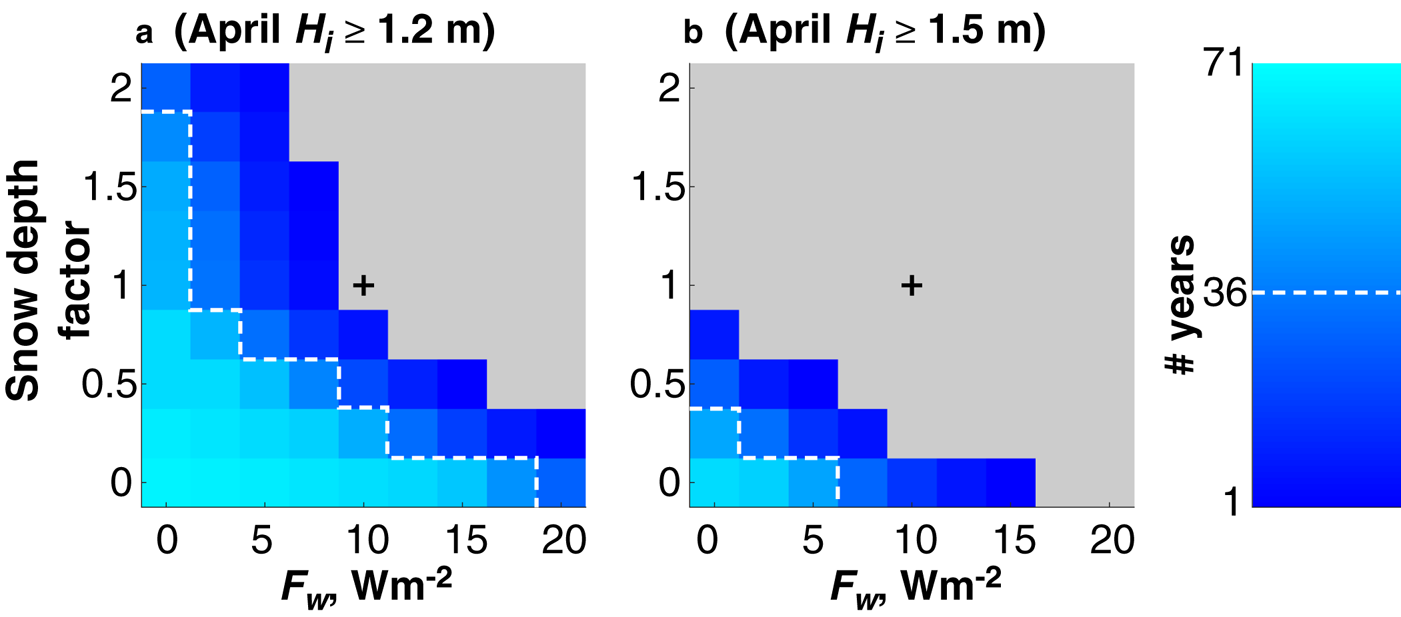
To understand the range of conditions that would have allowed the ice to typically achieve thicknesses of 1.2–1.5 m, we again used our growth model to simulate past ice thicknesses using historical air temperature data. Each year, we ran the model a total of 2025 times, allowing the freeze-up date, snow depth factor and ocean heat flux to vary each time. We specified an initial ice thickness of 0.1 m and allowed ice growth to start between 1 October and 28 January in 25 increments of 5 d. The snow depth factor varied between 0 and 2 in 9 increments of 0.25 and Fw varied between 0 and 20 in 9 increments of 0.25. We then identified the conditions that allowed at least 1.2 or 1.5 m of sea ice to grow by 1 April (Fig. 11).

Fig. 11. The number of years since 1945 during which ice thicknesses of (a) 1.2 m and (b) 1.5 m could have been achieved by 1 April and the combination of snow depth and ocean heat flux, F w, conditions that would have allowed this. The dashed white line circumscribes the conditions that would have allowed such ice growth more often than not (i.e. in >36 years). Grey areas indicate that the minimum ice thickness could not be achieved under such conditions. The black cross represents the conditions that prevailed in 2019.
The center of each panel in Figure 11 is marked by a plus-sign and corresponds to the snow depths and ocean heat flux that were observed or derived in 2019 (snow depth factor of 1 and F w = 10 W m−2). Under these conditions, our model indicates that it was not possible to grow 1.2 m in any year since 1945. The white dashed lines circumscribe the conditions under which the ice achieved thicknesses of 1.2 m (Fig. 11a) and 1.5 m (Fig. 11b) more often than not (i.e. in at least 36 out of the 71 years for which we have air temperature data). Our model indicates that achieving 1.2 m of ice more than half-time would have required either less snow or a lower ocean heat flux than in 2019. This thickness of ice could have been regularly achievable with more snow, but the heat flux would have had to zero. Similarly, if the heat flux were any higher, the snow depth would have had to be zero. There is an even narrower range of conditions required for growing 1.5 m of ice and our model suggests it would not have been possible with any more snow than was observed in 2019. For 1.5 m of ice growth to have occurred more often than not, our model suggests that the snow depth would have to have been less than half what was observed in 2019 and the mean ocean heat flux would have to have been <5 W m−2. Hence if these thicknesses were considered typical in the past, then the snow must have been shallower and the ocean heat flux must have been lower.
5. Conclusions
The work presented here is the product of a knowledge co-production approach (Behe and Daniel, Reference Behe and Daniel2018) designed to address the three research questions list in section 1, which integrate scientific and Indigenous knowledge systems. Although our results do not provide exhaustive answers, by framing our conclusions in response to each question, we can improve our understanding of the connections between the mass balance of landfast ice, marine mammals and subsistence hunting in Kotzebue Sound. In particular, if the unprecedented conditions documented in this study are indicative of years to come, then our findings detailed below may help inform adaptation strategies for subsistence activities and marine management. Regardless, co-production approach described here could serve as a template for designing future studies of sea ice in Kotzebue Sound and other coastal settings.
5.1 Research question I: what environmental factors control the length of the bearded seal hunting season in Kotzebue sound?
Our two MBSs in the landfast ice near Kotzebue measured ice growth and melt during the winters of 2017–18 and 2018–19, which turned out to be the two warmest winters on record since at least 1945. The winter of 2018–19 was both warmer and snowier than the winter of 2017–18 and, consequently the ice was thinner and began melting earlier. However, the anomalously high air temperatures and deep snow of the 2018–19 winter do not fully explain the lack of growth observed at our MBS. Using a 1-D ice growth model that accounts for surface flooding and the formation of snow ice, we estimate there was a continuous average vertical ocean heat flux, F w, in the center of the channel near Kotzebue of ~10 W m−2 from at least January to April in 2019. This heat flux reduced ice growth and caused bottom melt when it exceeded the conductive flux through the ice from the ocean to the atmosphere, F c. In both 2018 and 2019, F w was greater in the center of the channel than near its edge and increased toward the end of winter, reaching up to 30 W m−2 at the Channel MBS in 2019. We therefore conclude that heat from the water in the channel plays a significant role in the breakup of ice in the channel. This break-up is strongly connected to the start of the ugruk hunting season (Hauser and others, Reference Hauser2021, in press) and so years with a high ocean heat flux are likely to favor an early start to ugruk hunting in Kotzebue.
5.2 Research question II: what snow and ice surface properties promote ringed seal denning and pupping?
Although none of our Indigenous Advisory Council can recall finding flooded ringed seal lairs before, surface flooding is unlikely to promote denning and pupping success and is, instead, likely to have negative impacts on ringed seals whose dens become flooded. We observed flooding in both years at both MBS, and in 2018, we found a flooded seal lair near Sisualik (Fig. 1b). In all cases, we showed that the flooding was likely caused by the reduced buoyancy of the relatively thin underlying sea ice, and in 2019, the unusually deep snow pack. Our 1D model was able to accurately simulate the observed flooding by modifying the isostatic equation to account for the weight of water in the flooded snow (Eqn (11)). We are aware of only one other study that has adopted this approach (Kirillov and others, Reference Kirillov, Dmitrenko, Babb, Rysgaard and Barber2015) and our results are in agreement with theirs. Without accounting for wetting of the snow pack below the waterline, the standard isostatic equation applied for sea ice (e.g. Maksym and Jeffries, Reference Maksym and Jeffries2000; Zwally and others, Reference Zwally, Yi, Kwok and Zhao2008) underestimates flooding by at least half. The limited observations of flooded lairs in the scientific literature have been associated with lair abandonment or pup mortality (Lukin and Potelov, Reference Lukin and Potelov1978; Kelly and others, Reference Kelly, Quakenbush and Rose1986; Lukin and others, Reference Lukin, Ognetov and Boiko2006; Williams and others, Reference Williams, Nations, Smith, Moulton and Perham2006). In any case, accurate estimation of the amount and timing of surface flooding and the conditions that lead to it will be important for understanding any impact on ringed seal habitat.
Our observations at each MBS showed that snow ice formation resulting from surface flooding made a significant contribution to the total thickness of ice in 2019. Although the formation of snow ice was found to have a net positive contribution to the mass balance of the sea ice, the flooding of the snow contributed to increased bottom melt by effectively nullifying F c until the flooded snow was completely refrozen. If the ocean heat flux, F w ≫ 0, the depth of flooding can therefore increase over time even without additional snow through thinning of the underlying ice.
5.3 Research question III: why was there so little sea ice in Kotzebue Sound in 2018 (and 2019)?
Using the historical air temperature record to force our ice growth model, we demonstrated that not only were the winters of 2017–18 and 2018–19 the warmest since 1945, but the sea ice was also probably the thinnest to have occurred during this time. Our model indicates that for the landfast sea ice near Kotzebue to have been thinner than was observed in 2019 during any other winter since 1945, there would have needed to be a snow pack 50% deeper and an average ocean heat flux of 15 W m−2. We consider this unlikely, since 2019 was notable for having a deep snow pack and satellite-derived sea surface temperature data suggest ocean heat fluxes as high as we estimate in 2018 and 2019 are a recent phenomenon (Serreze and others, Reference Serreze, Barrett, Crawford and Woodgate2019). This is supported by further analysis of our model results that suggests both snow and ocean heat flux must have been lower in the past for conditions to favor frequent growth of ice up to 1.5 m thick, as reported by local Elders on our Advisory Council, who recall requiring longer augers to make ice fishing holes. Thus, we can address the third question from our Indigenous Advisory Council by concluding that an anomalous ocean heat flux probably contributed to the lack of ice that was first observed in 2018 and then again in 2019.
Acknowledgements
The research described in this publication is funded by the Gordon and Betty Moore Foundation through Grant GBMF5448 to Lamont-Doherty Earth Observatory of Columbia University. We are grateful to the Qikiqtaġruŋmiut people and the community of Kotzebue for sharing their Indigenous Knowledge and welcoming our research team. In particular, we wish to thank Pearl Goodwin, Siikauraq Whiting and Vernetta Nay Moberly for their support and generosity. We also thank Vincent Schaeffer for assistance with field activities and making and reporting mass-balance observations during 2019. Joshua Jones also provided field assistance in establishing the field sites in 2019. We also extend our gratitude to the Native Village of Kotzebue and the University of Alaska Fairbanks Chukchi campus who provided meeting facilities and the US Fish & Wildlife Selawik Refuge who provided housing. Historical meteorological data for Kotzebue airport were obtained from the National Centers for Environmental Information at https://www.ncdc.noaa.gov/cdo-web/datasets/LCD/stations/WBAN:26616/detail. Marine mammal research activities were conducted under National Marine Fisheries Service Permit # 19309. This is Lamont Contribution # 8488.
Author contributions
A.R.M. contributed to the design of the study and performed the majority of the analysis, synthesis and writing. K.E.T. designed, constructed and deployed the MBS equipment, performed the initial analysis of data and reviewed the manuscript. D.D.W.H., N.J.M.L., J.M.L., A.V.W. and C.R.W. assisted with the deployment of the MBS and other field observations and reviewed the manuscript. J.G., C.H., R.J.S. and R.S. comprise our Indigenous Advisory Council and contributed to the identification and design of research questions and the design of the field program. Each member of the Advisory Council also participated in fieldwork. R.J.S. and A.V.W. collected MBS data during the winter months. S.B. and A.S. contributed to the design of research questions, participated in fieldwork and reviewed the manuscript. C.J.Z. contributed to the design of research questions, reviewed the manuscript and is the lead investigator for the Ikaaġvik Sikukun project.


 Open access