Introduction
The microstructure of snow, i.e. the three-dimensional (3-D) configuration of the ice matrix, determines crucial snow properties, such as albedo, which is relevant for the computation of the surface energy balance, or mechanical strength for avalanche hazard forecasting and evaluation. The microstructure characterization based only on bulk parameters (e.g. density) is often insufficient to model precisely the mechanical and physical behavior of snow (Reference MellorMellor, 1975; Reference Shapiro, Johnson, Sturm and BlaisdellShapiro and others, 1997). A better understanding of the physical and mechanical snow properties requires a 3-D representation of the microstructure at a scale of a few microns (Reference Schneebeli and BrebbiaSchneebeli, 2002). Thanks to easier access to 3-D imaging facilities (e.g. X-ray computed microtomography) and increasing computational capabilities, 3-D images of the snow microstructure are now available. Numerical simulations directly based on the real 3-D microstructure of snow have been successfully applied to model thermal conductivity (Reference Kaempfer, Schneebeli and SokratovKaempfer and others, 2005; Reference Calonne, Flin, Morin, Lesaffre, Rolland du Roscoat and GeindreauCalonne and others, 2011), snow metamorphism (Reference Flin, Brzoska, Lesaffre, Coléou and PieritzFlin and others, 2003; Reference Brzoska, Flin and BarckickeBrzoska and others, 2008; Reference Flin and BrzoskaFlin and Brzoska, 2008) and mechanical properties (Reference Pieritz, Brzoska, Flin, Lesaffre and ColéouPieritz and others, 2004; Reference SchneebeliSchneebeli, 2004; Reference Srivastava, Mahajan, Satyawali and KumarSrivastava and others, 2010; Reference Theile, Löwe, Theile and SchneebeliTheile and others, 2011). Acquiring 3-D images of snow is therefore a key issue in snow research.
Different techniques can be used to capture the 3-D microstructure of snow, the most common being serial sectioning (Reference Perla, Dozier and DavisPerla and others, 1986; Reference GoodGood, 1987; Reference SchneebeliSchneebeli, 2001) and X-ray microcomputed tomography (μCT) (Reference BrzoskaBrzoska and others, 1999; Reference Coléou, Lesaffre, Brzoska, Ludwig and BollerColéou and others, 2001; Reference Freitag, Wilhelms and KipfstuhlFreitag and others, 2004; Reference Schneebeli and SokratovSchneebeli and Sokratov, 2004; Reference Chen and BakerChen and Baker, 2010). These methods differ in the way they reconstruct a 3-D volume from two-dimensional (2-D) data. Serial sectioning consists of an iterative slicing of the sample and 2-D imaging with an optical camera. μCT uses back-projection algorithms to obtain a spatial image from several radiographs recorded at different projection angles. μCT measures the 3-D distribution of the X-ray attenuation coefficient, which differs between materials with different chemical composition and density. Regardless of the imaging technique, the measurement output consists of a 3-D grayscale image, whose gray levels are supposed to be distinct between the different materials.
The material of interest then needs to be extracted from the grayscale image. This image-processing step is called binary segmentation. It consists of reducing the grayscale image to a binary image object/background, which enables the quantitative characterization of the microstructure. In the present case, the object of interest is ice and the background is generally constituted of air and possibly an impregnation product used to strengthen fragile snow samples. Unfortunately, the grayscale image is noisy and the transition between materials is generally fuzzy. Thus, the binary segmentation is not straightforward and might bias the microstructure characterization and the result of subsequent numerical models.
The segmentation technique used for snow is usually based on thresholding (e.g. Reference Coléou, Lesaffre, Brzoska, Ludwig and BollerColéou and others, 2001; Reference Flin, Brzoska, Lesaffre, Coléou and PieritzFlin and others, 2003; Reference Schneebeli and SokratovSchneebeli and Sokratov, 2004; Reference Kerbrat, Pinzer, Huthwelker, Gäggeler, Ammann and SchneebeliKerbrat and others, 2008; Reference Heggli, Frei and SchneebeliHeggli and others, 2009): single gray values are used to separate different materials. These methods based on thresholding are commonly used in the snow community because they are fast and their implementation is straightforward. However, they are not robust in practice (Reference Boykov and Funka-LeaBoykov and Funka-Lea, 2006), and are operator-biased because of the subjectivity involved in the choice of threshold values (Reference Iassonov, Gebrenegus and TullerIassonov and others, 2009).
Nowadays, numerous advanced segmentation techniques are available in computer sciences, benefiting from the increasing computational capabilities of personal computers (PCs). Reference Iassonov, Gebrenegus and TullerIassonov and others (2009) compared different segmentation techniques on μCT images and concluded that ‘the use of local spatial information is crucial for obtaining good segmentation quality’ . Therefore, global thresholding methods might not be suited to deriving the maximum information from the grayscale image. One class of segmentation relying on the optimization of some energy functions is particularly powerful (Reference Boykov and Funka-LeaBoykov and Funka-Lea, 2006). These methods are hereafter referred to as energy-based segmentation. In the comparison conducted by Reference Iassonov, Gebrenegus and TullerIassonov and others (2009), energy-based segmentation has been shown to be superior to the other tested segmentation techniques. The energy definition makes these methods flexible and explicitly specifies the segmentation criteria. In addition, global optimization via the graph-cut approach (Reference Boykov, Veksler and ZabihBoykov and others, 2001; Reference Boykov and Funka-LeaBoykov and Funka-Lea, 2006) makes these methods repeatable and robust. Here we propose to take advantage of the formalism of energy-based techniques and to adapt it to the binary segmentation of snow microtomographic images.
Energy-based segmentation techniques can benefit from the a priori knowledge that the segmented object is snow. Density and specific surface area (SSA) are classical indicators to characterize the microstructure and can be measured from snow samples using dedicated instruments independent of μCT-based techniques (Reference Matzl and SchneebeliMatzl and Schneebeli, 2006; Reference Kerbrat, Pinzer, Huthwelker, Gäggeler, Ammann and SchneebeliKerbrat and others, 2008; Reference Gallet, Domine, Zender and PicardGallet and others, 2009; Reference ArnaudArnaud and others, 2011). Threshold-based segmentation techniques can already take into account the density prior information by choosing the right threshold value, but this is the only information that can be added in the segmentation process. The energy-based segmentation is more flexible and can also consider local spatial image information such as curvature (Reference El-Zehiry and GradyEl-Zehiry and Grady, 2010), local smoothness (Reference Boykov and KolmogorovBoykov and Kolmogorov, 2003) and shape (Reference Freedman and ZhangFreedman and Zhang, 2005).
Once fallen to the ground, snow undergoes metamorphism (Reference FierzFierz and others, 2009). Under equilibrium conditions, it tends to evolve to a structure that minimizes its surface and grain boundary energy (Reference Flin, Brzoska, Lesaffre, Coléou and PieritzFlin and others, 2003; Reference Vetter, Sigg, Singer, Kadau, Herrmann and SchneebeliVetter and others, 2010). As a result, the ice surface of aged snow tends to be smooth below a certain spatial scale. Reference Kerbrat, Pinzer, Huthwelker, Gäggeler, Ammann and SchneebeliKerbrat and others (2008) compared the SSA measured by gas adsorption and X-ray tomography. Except for fresh snow, both measurements give identical results, with an uncertainty of 3%. They concluded that the ice surface in an alpine snowpack is essentially smooth up to a scale of ~30 μm which corresponds to the effective resolution of their X-ray images. Reference Flin, Furukawa, Sazaki, Uchida and WatanabeFlin and others (2011) estimated the SSA of snow using microtomographic images of various snow types. They compared the computed SSA for different image resolutions. For coarse rounded or melt-refrozen grains with a low SSA (<20m2 kg−1), the computed SSA is almost independent of the image resolution in the range [5, 80] μm. As a consequence, snow structures smaller than 80 μm do not contribute significantly to the overall SSA for these types of snow. Thus, we can expect aged snow or melt-refrozen snow with a low SSA to be globally smooth even at a scale of 80 μm. In this paper, we attempt to include this prior information about local smoothness, which is linked to the overall SSA, in the segmentation process.
First, the sampling and X-ray μCT measurement procedures used to obtain grayscale μCT images are described. The gray-level distribution is analyzed and used to explain why the measurement artifacts significantly complicate the segmentation process. Second, the threshold-based segmentation, commonly used in snow research, and the new proposed energy-based segmentation are presented. Finally, the segmentation techniques are applied on a 2-D reference image and on the μCT images of snow, and the results are compared.
X-Ray μCT Images
Sampling and μCT measurement procedure
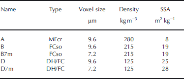
The natural snow samples used in this work were collected at Col de Porte, Chartreuse, French Alps, during winter 2011/12. Three different types of snow were sampled. Sample A is a melt–freeze crust (MFcr according to the International Classification for Seasonal Snow on the Ground (ICSSG; Reference FierzFierz and others, 2009)). Sample B is composed of solid faceted crystals (FCso) and presents a very fine crust of frozen drizzle. Sample D is composed of depth hoar (DH) and faceted crystals (FC). Density and SSA of these samples are summarized in Table 1.
Table 1 Description of the snow samples used in this study. Density was measured in the field by weighting snow samples with a volume of 50cm3. The indicative SSA values correspond to estimates obtained on the binary image resulting from the energy-based segmentation (for r = 1.0 voxel; see below)
The snow samples were prepared according to the procedure detailed by Reference Flin, Brzoska, Lesaffre, Coléou and PieritzFlin and others (2003) and Reference FlinFlin (2004). We only recall the main steps here. Once sampled in the field, each snow core was impregnated with liquid 1-chloronaphthalene (melting point −15/−20°C) at a temperature of −8°C. The ice/chloronaphthalene mixture was then allowed to freeze and stored in a refrigerator at −20°C. After complete freezing and strengthening, each sample was machined into the shape of a cylinder of 16 mm diameter and 21 mm height. This impregnation procedure enables handling of very fragile snow samples and blocks metamorphism of the snow structure.
The X-ray attenuation coefficient 3-D images were acquired with a cone beam tomograph (RX Solutions, generator voltage of 100 kV, generator current of 100 μA) using a specifically designed refrigerated cell. The image borders are slightly distorted due to the conic form of the X-ray beam. Thus, cubes of 10003 voxels were extracted from the inside of the whole 3-D grayscale images (~15003 voxels). The voxel side-length of sample A is 9.6 μm. Samples B and D were scanned twice with a voxel size of 7.2 μm (images B7m and D7m) and 9.6 μm (images B and D).
With this sampling procedure, the scanned samples present two main materials, namely ice and chloronaphthalene (chl), and a secondary material composed of residual air bubbles due to incomplete impregnation of the sample (Fig. 1). These three materials can be distinguished by their X-ray attenuation coefficient, i.e. their grayscale value I. The attenuation coefficients, initially encoded on 4-byte floats, were rescaled and encoded with unsigned shorts (0–65 535). In the figures, they are plotted with a gray level (0: black; 65 535: white). Dark, intermediate and light gray values correspond to air, ice and chl, respectively.
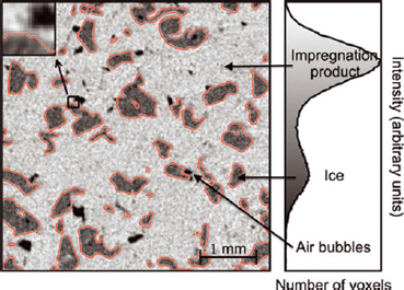
Fig. 1. X-ray scale image (5002 pixels) extracted from sample B, and its corresponding grayscale histogram. The image is composed of three materials: the impregnation product (1-chloronaphthalene, light gray), ice (intermediate gray) and residual air bubbles (dark gray). The contour of ice resulting from segmentation is plotted in red. The zoom box (top right) was enlarged five times to show the fuzzy transition between the different materials.
The segmentation method described in this paper is thus applied to X-ray images composed of three materials, resulting from snow samples impregnated with 1-chloronaphthalene. However, this approach is, in fact, rather general and can be applied to any multiple-material grayscale image from which one material needs to be extracted. Other sampling procedures to prepare snow samples for μCT imaging exist in the literature. When a μCT is directly available in a cold room, the snow samples generally do not require any specific preparation to be scanned (e.g. Reference Kerbrat, Pinzer, Huthwelker, Gäggeler, Ammann and SchneebeliKerbrat and others, 2008). In this case, the μCT image is composed of only two phases: air and ice. Besides the technique described in this paper, fragile snow samples can also be prepared for a μCT scan using the snow replica method (Reference Heggli, Frei and SchneebeliHeggli and others, 2009). This method consists of casting snow samples with diethyl phthalate and then sublimating ice in high vacuum. In this case, the scanned sample is composed of two materials: the impregnation product and air. In all cases, however, regardless of the reconstruction technique or the sampling procedures, the measurement output consists in a 3-D grayscale image whose values are supposed to be distinct between the different materials, and to which the developed segmentation technique can be applied.
Image artifacts: noise and fuzzy transition between materials
The μCT output images are only approximate representations of the true X-ray attenuation coefficient. The grayscale images are affected by optical transfer function, scatter and noise (Reference Kaestner, Lehmann and StampanoniKaestner and others, 2008). As a consequence, they are altered by two main artifacts: (1) the gray values of voxels belonging to the same material are slightly spread around the noiseless attenuation coefficient of the material, and (2) the transition between different materials is fuzzy (Fig. 1). These artifacts yield ‘mixed voxels’ whose gray value does not directly determine whether they belong to ice or to the background, and the segmentation of these mixed voxels can significantly affect the final segmented image. This explains why binary segmentation of μCT images is not straightforward.
The grayscale histogram representing the distribution of voxels with a given gray level (Fig. 2) can be used to estimate the material proportions and their intensity peaks. Its analysis can also be used to quantify the noise amplitude and the size of the transition zone between materials. Noise is inherent to the X-ray sensor and the measurement environment. Due to the acquisition method, noise is often spatially correlated along annuli centered on the rotation axis of the μCT scan. As shown in Figure 2, the noisy gray-level distribution for each material can be fitted by a Gaussian distribution ![]() , defined as
, defined as

The standard deviation σ and the mean μ of these distributions can be automatically determined using data adjustment algorithms (minimization of the square error), for ice and chl. Automatic fit for air is generally not possible because the amplitude of the air peak is too small to clearly emerge in the histogram. As expected, it is found that the standard deviation of noise is the same for chl and ice, since noise does not depend on the material but is inherent to the imaging procedure. The fitting domain was thus reduced by using the same σ value for ice and chl. In the example images (Figs 1, 3 and 10), the value of this standard deviation of noise σ is ~20% of the contrast between the attenuation coefficients of ice (μ ice) and chl (μ chl).
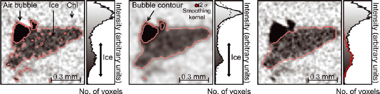
Fig. 3. (a) Threshold-based segmentation without smoothing. The thresholds used are indicated by the black arrow on the histogram. (b) Threshold-based segmentation with smoothing of the grayscale image through a Gaussian filter (σ s = 1.6 pixels). To visualize the size of the smoothing kernel, a disk of radius σ s voxels is plotted in red. The histogram of the non-filtered image is plotted with dots. (c) Expected segmentation (best segmentation obtained with the energy-based technique). The grayscale distribution ofthe segmented ice pixels is plotted in red on the histogram. Despite the clear visual differences, the threshold-based segmentation without smoothing (a) differs from this expected segmentation (c) by only a small number of voxels (~5%).
The fuzzy transition between different materials is partly due to partial volume effect (Fig. 1). The real limit between materials does not exactly follow the voxel grid. Therefore, the gray value of a frontier voxel is a barycenter between gray values of pure materials. In principle, the transition width should thus be on the order of the voxel side-length. In fact, this zone is slightly larger (~2–3 voxels). This is due to the tomography back-projection reconstruction algorithm that is affected by a noisy input. On the histogram, this effect leads to a transition zone between ice and chl (Fig. 2). Empirically, a Gaussian distribution centered on the mean gray level ![]() and with a standard deviation of
and with a standard deviation of ![]() was found to provide a good fit to this transition zone (Fig. 2).
was found to provide a good fit to this transition zone (Fig. 2).
Hence, the normalized grayscale histogram F can be well reproduced by the following model ![]() :
:
where (λ ice, λ chl) represent the proportions of ice and chl, respectively. As a consequence, the undetermined voxels whose gray value is between ice and chl are either very noisy pure material or transition voxels between the two materials. As described below, this automatic histogram analysis is used to set the parameters of the energy-based segmentation algorithm.
Method
Various binary segmentation methods have been proposed in the literature (Reference Boykov and Funka-LeaBoykov and Funka-Lea, 2006; Reference Iassonov, Gebrenegus and TullerIassonov and others, 2009). In the snow community, global thresholding with pre- and post-processing smoothing filters is commonly used (e.g. Reference Coléou, Lesaffre, Brzoska, Ludwig and BollerColéou and others, 2001; Reference Flin, Brzoska, Lesaffre, Coléou and PieritzFlin and others, 2003; Reference Schneebeli and SokratovSchneebeli and Sokratov, 2004; Reference Kerbrat, Pinzer, Huthwelker, Gäggeler, Ammann and SchneebeliKerbrat and others, 2008; Reference Heggli, Frei and SchneebeliHeggli and others, 2009). This threshold-based segmentation method and its drawbacks, which have motivated the development of a more advanced segmentation method, are first described. The proposed energy-based segmentation is then presented.
Threshold-based segmentation
Threshold-based segmentation is the most commonly used segmentation technique because it is simple and fast. The method is based on two main steps: smoothing and thresholding. These steps differ depending on whether the image is composed of two or more phases.
Two materials
During the thresholding process, individual voxels in the image are marked as objector background voxels according to whether their value is greater or smaller than a global threshold value. This threshold can be estimated from the grayscale histogram of the image. For instance, its value can be determined as the local minimum between the two intensity peaks in the grayscale histogram (Fig. 1; e.g. Reference Heggli, Frei and SchneebeliHeggli and others, 2009). However, for snow samples with a very high SSA, these two peaks are not distinct (unimodal histogram) because of the large number of mixed voxels whose grayscale value lies between those of the two materials. In this case, the threshold can be determined by fitting a particular intensity model. For instance, Reference Kerbrat, Pinzer, Huthwelker, Gäggeler, Ammann and SchneebeliKerbrat and others (2008) determined the optimum threshold by fitting a sum of two Gaussian curves on the histogram and calculating their intersection. Nevertheless, using a strict gray threshold generally truncates the tail distribution of the intensity distribution of pure material voxels and results in a number of incorrectly classified voxels (Reference Kaestner, Lehmann and StampanoniKaestner and others, 2008; Fig. 3). The number of wrongly segmented voxels is particularly large when the histogram is unimodal. The resulting segmented object is thus disturbed, and structural parameters such as SSA are significantly affected.
In order to smooth the ice/background interface and to accentuate the intensity peaks in the histogram, a smoothing filter that reduces noise is first applied on the initial image. Common smoothing filters are convolution filters such as mean and Gaussian filters. The spatial size σ s of the smoothing filter (box size of the mean filter or standard deviation of the Gaussian filter) is usually set to the size of a few voxels. These filters efficiently smooth intensity variations inside homogeneous regions but also affect sharp features in the image. Consequently, the effective resolution of the binary image is negatively affected. Moreover, setting the size of the smoothing filter σ s to a certain value does not guarantee that the segmented object is free of artificial details smaller than σ s (Fig. 3) because the thresholding applied afterward is a discontinuous operation.
Three or more materials
When the initial image is composed of three or more materials, the smoothing step is not directly applicable. For instance, a smoothing filter directly applied on our X-ray images smooths the transition between air bubbles and 1-chloronaphthalene. The contour of air bubbles in chl then appears as an ice contour (Fig. 3b). The image therefore has to be reduced to a two-materials image before applying the smoothing/thresholding steps.
A semi-automatic threshold-based segmentation procedure was developed to process X-ray images of impregnated snow obtained from synchrotron tomography (Reference Flin, Brzoska, Lesaffre, Coléou and PieritzFlin and others, 2003; Reference FlinFlin, 2004). This approach was recently improved and now consists of the following steps:
Air bubble detection. First, a threshold is used to locate dark voxels corresponding to air. These voxels are then dilated (two iterations) where the grayscale gradient is high. This procedure enables labeling of the contour of air bubbles that have the same gray value as ice. Dilating only in high-gradient zones prevents labeling of real ice next to a bubble that is touching ice. Finally, the labeled voxels are replaced by the mean gray value of 1-chloronaphthalene. This step reduces the initial image to two materials.
Smoothing and thresholding. The modified image is smoothed with a mean filter of size 3 × 3 × 3 and binarized with a threshold obtained from a visual analysis of the grayscale histogram.
Final processing. To remove residual noise, the segmented image is post-processed via binary morphological operations (closing, erosion/reconstruction, opening, etc. with structural elements of size 3 × 3 × 3) and via a last smoothing/thresholding step (mean filter of size 5 × 5 × 5). Finally, ice zones not connected to the main structure or to the borders of the image are identified using a connected component- labeling algorithm and deleted. This step prevents having small artificial ice zones floating in the snow structure.
This procedure is straightforward and fast (~1–2 hours on a PC (2 GHz, 16 Gb RAM) for a 10003 voxels image). Nevertheless, its outcome critically depends on the skills of the operator, who has to manually fix the different segmentation parameters (thresholds, smoothing filters size, etc.) as a function of the snow type and the tomograph settings. Moreover, due to the sequential nature of the segmentation procedure, information might be lost between each smoothing and thresholding step. For instance, the initial smoothing step affects the whole image and does not preserve sharp edges. On the contrary, it tends to increase the partial volume effect. Lastly, the parameters used cannot be directly related to the effective resolution of the resulting binary image, i.e. the size of the smallest details that can be imaged.
Energy-based segmentation
Energy-based segmentation methods consist of finding the optimal segmentation according to an energy function. These methods are more robust because the segmentation criteria are objectively defined in the energy functional and the optimization process is automatic. Energy-based segmentation methods can be distinguished by the type of function used and by the minimization algorithm. They can be divided into two main groups (Reference Boykov and Funka-LeaBoykov and Funka-Lea, 2006):
-
1. Optimization of a functional defined on a continuous contour or surface (e.g. snakes, geodesic active contours, methods based on level-sets). The optimization generally uses a variational approach that finds a local optimum, but cannot guarantee to find a global optimum.
-
2. Optimization of a cost function directly defined on a discrete set of variables (e.g. intelligent scissors, live-wire, graph cut). The graph-cut approach introduced by Reference Boykov, Veksler and ZabihBoykov and others (2001) belongs to this group and enables the global optimization of the energy function in any dimension. In this paper, the graph-cut approach was adapted to the binary segmentation of snow X-ray microtomographic images.
Let us consider that the grayscale image I is constituted of n voxels of side length δ. The spatial position and the intensity of voxel i are denoted xi and Ii , respectively. The segmented image is L ∊ {0,1} n , where 0 stands for the background and 1 for ice. Li is the segmentation label (0 or 1) of voxel i. A segmentation L costs the energy E(L). The best segmented image L min is the one that minimizes the energy E. In general, the energy E is composed of two terms: a local data fidelity term (E v) and a non-local spatial regularization term (E s), whose expressions in our case are described in the following subsections.
Local intensity model
The local gray value is the most obvious criterion that needs to be accounted for in the segmentation process. For instance, a voxel whose intensity is very close to the intensity of air is inclined to be air, i.e. to belong to the background. This idea can be formalized with proximity functions P that quantify the penalty of assigning a voxel to ice or to the background. The proximity function ranges from 0 (furthest) to 1 (closest). Using proximity functions, the data fidelity term E v of the segmentation energy can be defined as
where P
0 is the proximity to the background (0), and P
1 the proximity to ice (1). This energy is scaled by the volume of 1 voxel v = δ3. To set these proximity functions, we rely on the analysis of the grayscale distribution (see above and Fig. 2). Using the decomposition of the grayscale histogram described in Eqn (2), the ratio ![]() quantifies ‘how close to ice a voxel of a given gray value level is’ and could be used as the proximity function to ice P
1. Here a simpler model that approximates this ratio based on truncated Gaussian functions is used (Fig. 4):
quantifies ‘how close to ice a voxel of a given gray value level is’ and could be used as the proximity function to ice P
1. Here a simpler model that approximates this ratio based on truncated Gaussian functions is used (Fig. 4):
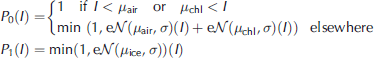
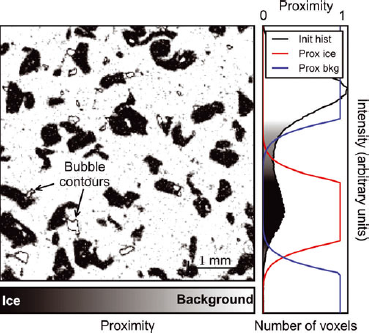
Fig. 4. Proximity image. The gray value is here proportional to P 0 − P 1, so that a voxel close to the background is white and a voxel close to ice is dark. The voxels with an intermediate gray value are the undetermined voxels. The contours of air bubbles are visible. The same plot can be done with a preprocessed image where the bubble contours are replaced by chl, but then a peak appears in the histogram for the chosen ‘replacement’ intensity.
with e = exp(1). The attenuation coefficient of air, μ air, cannot be directly derived from the histogram. This parameter is estimated from the values of μ ice and μ chl by assuming a constant relative contrast between materials. Using these proximity functions actually amounts to transforming the initial grayscale image into a new grayscale image (Fig. 4), which is sharper because the noise has been reduced. The main idea behind this definition of the proximity functions is to distinguish the fuzzy transition from noise and add this information to the segmentation process.
Even if no smoothing filter is applied to the grayscale image, the contour of air bubbles generally shows gray values close to those of ice, due to the partial volume effect (Figs 3 and 4). To eliminate this artifact, ‘ice-like’ (μ ice − 2σ < I < μ ice +2σ) voxels, simultaneously close (distance 4 voxels) to ‘chl-like’ (I >μ ice − σ) and ‘air-like’ (I < t μ air + σ) voxels, are replaced by ‘chl-like’ voxels (I = μ chl − σ). All μCT images used to test the energy-based segmentation method were preprocessed this way.
The minimization of E v alone gives the same result as a threshold-based segmentation, with the advantage of also providing the uncertainty of the segmentation E v(L min). However, the energy-based segmentation is really interesting when E v is combined with additional non-local energy terms.
Surface area
The complete energy function used in this paper is composed of two components:
where the spatial regularization term is E s(L) = r · S(L), with S(L) the surface area of the segmented object and r (r ≥ 0) which has the dimension of a length. Accounting this term in the energy leads to penalizing large interface areas: a voxel with a mixed gray value will be segmented so that the interface ice/background area is minimized. The parameter r assigns a relative weight to the surface area term so that the smoothness of the segmented ice can be controlled. In principle, other non-local terms (e.g. gradient, curvature or shape penalties) could also be considered in the segmentation. The flexible definition of the energy functional is one of the powerful assets of energy-based segmentation.
The regularization term minimizing the ice/air interface is of particular interest for materials such as snow where sintering naturally tends to reduce the surface and grain boundary energy. This process is particularly effective on snow types resulting from isothermal metamorphism. For other snow types, such as precipitation particles (PP), faceted crystals (FC) or depth hoar (DH), the surface regularization term is expected to perform well in recovering the facet shapes but might induce some rounding at facet edges.
The parameter r is a geometrical parameter related to the smallest detail size preserved by the segmentation. Let us consider a protuberance P on a globally smooth interface, with a volume V p, a total surface S p and a contact area with the smooth object S c (Fig. 5). If P is considered as ice, the segmentation energy is E = C + r · (S p − S c) where C is a constant. If P is considered as background, then E = C + V p + rS c. Hence, the protuberance P is segmented as ice if
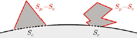
Fig. 5. Protuberances on a surface of a smooth object. For the equilateral triangular protuberance, α = 1/3. For the ‘sharper’ protuberance, α = 0:8.
In addition, the contact area S c can be generically expressed as a function of the total surface area S p: 2S c = (1 − α)S p where α is a numerical factor that depends on the protuberance shape. This factor α ranges from 0 to 1 for flat to distinct protuberances, respectively. For instance for an equilateral triangle protuberance, α = 1/3. Let r p be an apparent radius, defined by V p /S p. Finally, P is segmented as ice if
Accordingly, the segmentation parameter r thus enforces the minimum radius of protuberances preserved on the segmented object.
Minimization of the energy: graph-cut approach
The energy functional defined in Eqn (5) has to be minimized to find the optimal segmentation. The optimization of binary energy via graph cut is well suited to this purpose (Reference Boykov, Veksler and ZabihBoykov and others, 2001). This method consists in transforming the binary energy optimization problem into the problem of finding an optimal cut in a graph, which is solvable in polynomial time (Reference Ford and FulkersonFord and Fulkerson, 1956). The cut metric induced in this graph can be chosen as close as desired to the continuous Euclidean metric (Reference Boykov and KolmogorovBoykov and Kolmogorov, 2003) and can also be used to compute surface area very efficiently (Reference Lehmann and LeglandLehmann and Legland, 2012). Details of the graph-cut approach are provided in the Appendix. The graph-cut algorithm developed by Reference Delong and BoykovDelong and Boykov (2008) that enables the segmentation of massive grids up to 4003 voxels on a PC was used. Since segmentation is a local process at the scale of a snow grain, it was possible to apply a ‘divide and conquer’ (D&C) algorithm (segmentation on smaller overlapping sub-volumes) in order to segment large images (~10003 voxels) in ~10 hours on a PC (four processors, 2.7 GHz, 6 Gb RAM).
Results
The absence of ground truth, i.e. the absence of prior knowledge of the optimal binarization result, makes the comparison of different segmentation techniques difficult. Thus, the accuracy and the behavior of the energy-based segmentation is first tested on a reference artificial image: the 2-D Koch flake. The technique is then applied on μCT snow images, and 3-D results are shown. Results of the energy-based and threshold-based segmentations are compared, and the accuracy of the energy-based segmentation is indirectly checked on global structural parameters (density and SSA).
Segmentation of a reference 2-D image
The Koch flake (Fig. 6) is chosen as a reference for its multiscale properties (Reference MandelbrotMandelbrot, 1982) that can grossly mimic the structure of certain types of snow. By varying the number of iterations in the fractal construction, the scale of the smallest detail on the flake can be freely set, and the exact perimeter length and surface area can be theoretically computed. First, the discretization of the Koch flake into a pixel binary image is discussed. This binary image is then artificially degraded to reproduce the imperfect μCT output image. Finally, the energy-based segmentation method is applied on the degraded image and its accuracy is examined.
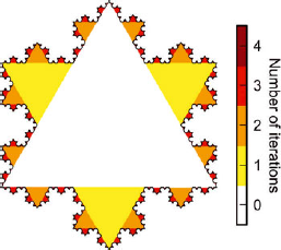
Fig. 6. Koch flake with four iterations (5002 pixels). At each iteration, a smaller triangle is added in the middle of all perimeter segments.
Discretization artifact
The flake is discretized into a binary image of size 5002 pixels: the value of each pixel was set to 1 or 0 according to whether the pixel center is inside or outside the closed Koch curve, respectively. Figure 7 shows measurements of the area and the perimeter (computed with the graph-cut approach: see Appendix) of the discretized Koch flake as a function of the iteration number in the construction of the fractal object. The measured area corresponds well to the theoretical value. The measured perimeter, however, differs more and more from the theoretical value when the number of iterations increases, i.e. when the length of the elementary segment of the Koch curve becomes small compared to the pixel size. Typically, the perimeter measurement remains consistent with the theoretical value, with an uncertainty of 10%, for objects whose details are larger than ~4 pixels. For smaller details, discretization artifacts become significant; in this case, the pixel discretization and the graph-cut length calculation are not precise enough to correctly reproduce the flake contour length. In the following, the Koch flake with four iterations, which presents the smallest details of side-length equal to 4 pixels and whose contour length can be regarded as correctly reproduced, is considered as the reference object.
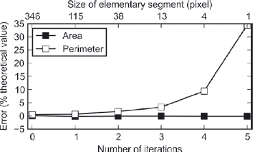
Fig. 7. Measurement of area and perimeter of the discretized Koch flake as a function of the number of iterations in the fractal construction (see Fig. 6).
Input images for the segmentation algorithm
The discretized Koch flake with four iterations was then blurred with a Gaussian filter of standard deviation equal to 1.5 pixels in order to reproduce the fuzzy transition between two materials (blurred image). Two synthetic images were then created by adding different types of noise to the blurred image. On the first one (CT noise image), noise derived from a CT scan of an empty sample was added to the blurred image, in order to mimic μCT noise as closely as possible (Fig. 8). On the other one (Gaussian noise image), uncorrelated Gaussian noise was added. Both additive noises were scaled so that their standard deviations are equal to 20% of the contrast between the two materials, as in our snow μCT images. Note that the specific surface area (SSA) of the Koch flake expressed in pixels is relatively small compared to that of the scanned snow grains since the center of the Koch flake is massive. Thus, only a small number of transition pixels are present, as revealed by the grayscale histogram (Fig. 8).

Fig. 8. Koch flake blurred with a smoothing filter (σ s = 1.5 pixels) and degraded with noise extracted from an empty CT scan. The CT-scan noise presents circular spatial correlations due to the data acquisition procedure.
Segmentation artifact
The energy-based segmentation algorithm was applied to the initial image and the degraded images (blurred, CT noise and Gaussian images) for various values of the parameter r. Note that the blurring of the initial image irreversibly affects details of the Koch flake which therefore cannot be recovered by any segmentation technique. Hence, the segmentation of the CT and Gaussian noisy images is expected to be, at best, as good as the segmentation of the blurred image.
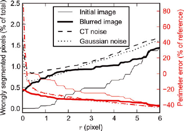
Figure 9 shows the number of pixels that are wrongly segmented compared to the reference Koch flake image, as a function of the segmentation parameter r. For both noisy images, the lowest number of wrongly labeled pixels (equal to 0.84% of the total number of pixels with the CT noise and 0.66% with Gaussian noise) is obtained with r = 0.4 pixel. As explained above (Eqn (7)), r controls the apparent radius of surface protuberances deleted by the segmentation. The optimal value of r is obtained when protuberances induced by noise are deleted but as few object details as possible are smoothed. Therefore, the optimal value of r can be regarded as corresponding to the typical length of noise-induced protuberances. Globally, the segmentation result is more accurate on the image with Gaussian noise, which can be attributed to the effect of spatial correlations of the μCT noise that tends to hinder the efficiency of the non-local segmentation energy term (E s).

Fig. 9. Accuracy of the segmentation on the Koch flake image as a function of parameter r. The reference perimeter is the perimeter measured on the discretized flake with four iterations (Fig. 7).
Figure 9 also shows how the perimeter length of the segmented object varies with r. As expected, when r increases, the perimeter becomes smoother and its length decreases. Two regimes can be distinguished: (1) For small values of r, the perimeter length strongly decreases with r. Due to noise, the length computed with r = 0 is highly overestimated. In this regime, smoothing induced by E s affects small details that are due to noise, but not real details of the image. (2) For larger values of r, the computed perimeter length decreases more slowly with r, and with a quasi-constant slope. In this regime, the smoothing induced by E s affects real details of the object. This is indicated by the fact that the computed perimeter length on the images without noise (initial and blurred images) also clearly decreases in this regime. Interestingly, the perimeter decrease rates with r for the noisy images and the blurred image are almost equal, and presumably linked to the multiscale property of the segmented object. Note that for very large values of r, the smoothing is so strong that there are almost no more differences between the results obtained from the four images (Fig. 9).
Interestingly, we observe that the segmentation with the smallest number of wrong segmented pixels is obtained at the transition between the two previously described regimes, i.e. when most noise induced by artificial details is smoothed out. We also note that the best segmentation is not able to recover the exact Koch flake: ~1% of the total number of pixels are wrongly segmented and the perimeter length is underestimated by 20% compared to the perimeter length computed directly on the initial image. As already explained, this discrepancy is mainly due to the application of blur, which leads to an irrecoverable loss of the smallest details in the image. It is thus satisfactory to observe that the perimeter length recovered by the best segmentation on the noisy images is almost equal to that obtained with the best segmentation (r = 0) on the blurred image.
Segmentation of snow 3-D images
The energy-based segmentation algorithm is now applied on the snow samples described previously (Table 1) for various values of segmentation parameter r. Examples of segmented slices (Fig. 10) and segmented volumes (Fig. 11) qualitatively illustrate the effect of parameter r on the segmented object. It is clearly observed that when r increases, the segmented snow becomes smoother and smoother. The effect of r is all the more evident for snow presenting a high SSA value (sample D).
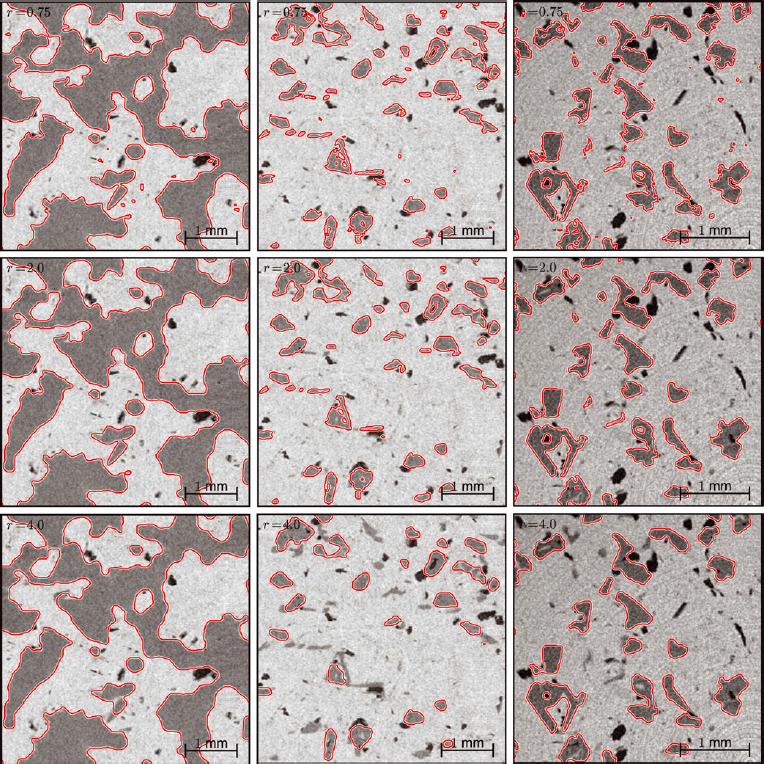
Fig. 10. Segmentation for different snow samples (A, D and D7m from left to right) and parameter r (0.75, 2.0 and 4.0 voxels from top to bottom). The segmentation is computed on a 3-D volume. As a consequence, the segmentation presented on these 2-D sub-slices (5002 pixels) may be affected by neighboring slices.
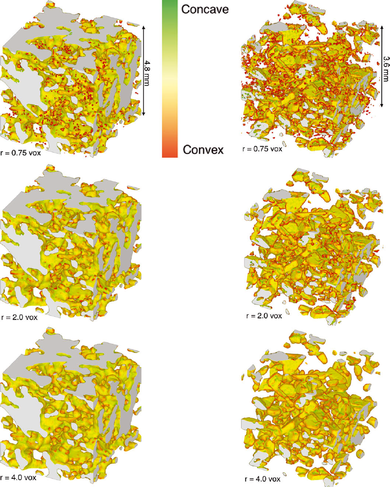
Fig. 11. Segmentation for different snow samples (A on the left and D7m on the right) and parameter r (from top to bottom 0.75, 2.0 and 4.0 voxels). The segmentation is presented on subvolumes (5003 voxels) of the whole images (10003 voxels) and may be affected by neighboring slices. The surface was colored according to its curvature to emphasize the smallest structure details.
In the following, we first investigate how the segmentation parameter affects structural variables such as density and SSA (Fig. 12). The results obtained for similar snow samples scanned with different resolutions are then compared. Finally, the energy-based segmentation results are compared to the threshold-based segmentation results.
Evolution with parameter r
As shown in Figure 12a, the density of the segmented object is almost constant with r. The slight decrease observed is due to the fact that the snow structure is generally convex and accounting for E s in the segmentation energy tends to erode convex zones. The density variations are also slightly larger for small snow grains (samples D and D7m) since their details are more affected by smoothing induced by E s (Fig. 10).
SSA, by contrast, is more sensitive to the segmentation parameter r (Fig. 12b). As for the Koch flake, two regimes can be distinguished. For very low values of r (0–10 μm), the SSA decreases rapidly when r increases. Similarly to the synthetic images, this regime probably corresponds to the progressive smoothing of the noise on the interface. For larger values of r (10–40 μm), the SSA decreases much more slowly with r. For sample A, composed of a melt-refrozen crust, there is actually almost no variation of the SSA with r in this regime, which can be related to the fact that the interface is already naturally smooth at these scales. For samples B and D, the SSA continuously decreases with r with an almost constant slope, because the real details of the snow structure contributing to the overall SSA are progressively smoothed out. This behavior is a clear indication of the multiscale characteristics of these types of snow: the wide size distribution of the details impacts the SSA when computed at different scales.
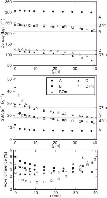
Fig. 12. Evolution of segmentation results as a function of the segmentation parameter r. (a, b) The evolution of density (a) and specific surface area (b) as a function of r. Density and SSA values obtained from the threshold-based segmentation are indicated on the right axis. (c) The proportion of voxels that differ between the energy-based and threshold-based segmentations.
Hence, when the scale of noise is clearly separated from the detail scale as on sample A, the segmentation parameter can be almost indifferently taken in the range 10–40 μm. When these two scales are not clearly separated, the optimal choice for r is more difficult. The best segmentation is obtained when most of the noise is smoothed out but the snow details are optimally preserved. According to the analysis of the Koch flake, we can assume that the best segmentation parameter is obtained at the transition between the two described regimes, i.e. when the SSA starts to vary slowly with r. In the presented images, this optimal value corresponds to r ≃ 10−15 μm, i.e. r ≃ 1−1.5 voxels. As expected, choosing a value of r less than this optimal value amounts to trying to extract artificial information from the image and to amplifying the influence of the noise. In our case, finding an optimal value on the order of the voxel size indicates that the tomograph settings are optimal.
Influence of image resolution
Segmentation results can be compared for the pairs of images B and B7m, and D and D7m, which were obtained using different resolutions (9.2 and 7.6 μm, respectively). For both density and SSA, the segmentation results are globally consistent with each other for all values of r larger than the highest resolution (Fig. 12). We recall that, even if they are extracted from the same sample, the volumes scanned at different resolutions are not exactly the same. This might explain the small density and SSA differences observed. The agreement observed for both pairs of images constitutes a clear validation of the robustness of the presented method. The parameter r can be regarded as the effective resolution of the segmented image.
For images B and B7m, both SSA and density values remain similar for values of r less than 9.2 μm. This indicates that, in this case, both resolution values are sufficient to capture the details of the tested snow type. By contrast, for images D and D7m, the SSA values tend to show a difference that increases when r decreases below 9.2 μm. This can be attributed to the influence of snow details smaller than the image resolution whose existence is expected for this type of snow with a high SSA value. The observed difference can also be enhanced by the slightly poorer quality of the D7m scan where the noise-to-signal ratio is larger.
Comparison with threshold-based segmentation
Globally, as shown in Figure 12c, the number of voxels differing between the two segmentation techniques always remains relatively small (1–5%). In detail, this number slightly depends on the considered image.
Concerning the density, it can be argued that good agreement between the two segmentation techniques is found for all tested images (Fig. 12a). The differences observed in Figure 12a can be attributed to the uncertainty inherent to the segmentation technique. For instance, a detailed investigation conducted on image A revealed that the differences between the two techniques are essentially due to systematic variations of ~1 voxel in the position of the ice/background interface (Fig. 13). Given the typical size of the fuzzy transition between materials in our image, such variations of 1 voxel may be due to slight differences in the chosen thresholds and can be regarded as measurement uncertainties. Due to the connectivity test, some snow grains also tend to be deleted in the threshold-based segmentation (Fig. 13), but their effect on the overall density remains negligible. Finally, it can also be noted that the density values measured in the field (Table 1) are in reasonable agreement with the values derived from the binary images, considering once again the measurement uncertainties, and the representativity issues linked to the small size of the scanned samples.
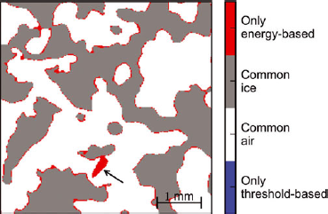
Fig. 13. Differences between the threshold-based segmentation and the energy-based segmentation computed for r = 2.0 voxels on a slice of sample A (5002 pixels). The grain indicated with the arrow was disconnected from the overall snow structure by the threshold-based technique and deleted by the connectivity test. Almost no blue pixel, which is segmented as ice only with the threshold-based method, is visible in the figure. On the threshold-based segmented image of sample A, a one-voxel dilation increases the computed density from 278 kg m−3 to 294 kg m−3, a value close to that obtained with the energy-based segmentation (Fig. 12a).
Concerning SSA, we also observe good agreement between the values derived from the threshold-based segmentation and those obtained from the energy-based segmentation, in particular when parameter r is on the order of the image resolution (Fig. 12b). This comparison reveals that the effective resolution associated with the threshold-based segmentation is actually close to the image resolution. Note that the apparently large difference in SSA values yielded by the threshold-based segmentation for images D and D7m is actually essentially due to the difference in the obtained densities and not in the obtained surface areas (Fig. 12a).
Energy-based and threshold-based segmentation have been shown to produce essentially identical results, which can be considered as a cross-validation of the two techniques. However, the threshold-based technique appears less robust since, in particular, different density values are obtained for the same samples scanned at different resolutions. The greater robustness of the energy-based technique is supported by the fact that the segmentation parameters are automatically derived from the histogram analysis, and not subjectively chosen as in the threshold-based segmentation. This robustness is also enhanced by the greater flexibility offered by the use of smooth proximity functions instead of fixed threshold values that separate voxels regardless of the grayscale difference between them.
Conclusion and Discussion
We successfully applied an energy-based segmentation with a graph-cut minimization technique, to snow microtomographic images. The segmentation criteria are chosen according to our prior knowledge of the snow microstructure. In particular, a spatial regularization term, that penalizes large interface area, has been introduced to account for the sintering effect that naturally tends to reduce snow surface energy.
Our approach has first been shown to produce accurate results on a synthetic image, the Koch flake. The energy-based segmentation was then successfully applied on microtomographic images of snow and compared to the threshold-based segmentation. In the absence of ground truth on snow images, it is difficult to conclude about the absolute quality of the obtained segmentations. However, both methods produced similar results. The main advantages of our approach compared to the threshold-based segmentation can be summarized as follows:
-
1. All segmentation parameters (intensity peaks, noise amplitude, etc.), except the relative weight of the surface area term r, are automatically determined from the histogram analysis in which both noise and fuzzy transition are considered. Thus, the approach is reproducible and does not involve subjective choices.
-
2. The method benefits from local spatial information: voxels are segmented according to their local gray value but also such as to minimize the ice/background interface, which is physically meaningful. The segmentation parameter r is formally linked to the local smoothness of the segmented object. It clearly defines the effective resolution of the final binary image.
-
3. With the energy formalism and the global optimization via graph cut, all criteria and available information are treated simultaneously in the segmentation process, which leads to enhanced robustness. In the threshold-based segmentation, the image processing is sequential. At each step, the ‘working’ image is modified and some information might be lost.
The density of the segmented image has been shown to be almost independent of parameter r. Thus, density values are essentially governed by the volumetric term in the segmentation energy. As a consequence, an a priori knowledge of the density might be added in the segmentation process. This can be done by adding this constraint to the histogram analysis phase and adjusting the values of μ air, μ ice and μ chl. In our case, such an addition of prior information was not considered since the density field measurements cannot be regarded as representative for the small scanned snow samples.
The choice of the segmentation parameter value r is not automatic and should be made according to the image quality. As shown previously, the best segmentation, i.e. that which preserves the smallest snow details while deleting most of the noise-induced protuberances, is obtained when the computed SSA starts to vary slowly with r (r ≃ 1−1.5 voxels here). The dependence of the computed SSA value on the effective resolution r also points to two important considerations: (1) if they are not carefully smoothed out, noise-induced protuberances can significantly contribute to the overall SSA, which will then be overestimated; and (2) for snow with structure details on the order of the voxel size (e.g. fresh snow), the SSA value cannot be measured independently of the resolution used.
In addition, the choice of r should also depend on the subsequent use of the binary image. For analyses not affected by small structural details, the effective resolution r of the binary image can be chosen larger than the optimal value defined above. For instance, for mechanical analysis with finite or discrete elements, the segmentation should correctly reproduce the grain connectivity while modeling the grain shapes with the fewest elements possible. Usually the downscaling of the 3-D image of snow is performed by merging voxels in the binary image. This downscaling leads to a threshold uncertainty when exactly half the subvoxels belong to ice or to the background. The downscaled image is therefore grid-dependent. The energy-based segmentation presented here has the advantage of enabling the effective downscaling of the 3-D representation of snow to a chosen resolution represented by the segmentation parameter r, without any grid artifact.
Acknowledgements
Funding by the VOR research network (Tomo FL project) and the European Feder Fund (projects Interreg Alcotra MAP3 and RiskNat) is acknowledged. We thank the scientists of 3SR laboratory (J. Desrues, P. Charrier and S. Rolland du Roscoat), where the 3-D images were obtained. We also acknowledge the CEN (Centre d’ Etudes de la Neige) staff (P. Pugliese and J. Roulle) for technical support during the experiments. Special thanks are due to N. Calonne for her significant contribution to the data acquisition. Irstea is a member of Labex 05UG@2020 and TEC21.
Appendix
In this appendix, the implementation of the segmentation energy and its optimization via graph cut is detailed.
Link between graphs and binary energy
Graph cut can be used to minimize binary energies. A binary energy is a function of a finite set of binary variables. For instance, the segmentation energy defined in Eqn (5) is a binary energy whose binary variables are the ice/background label of each voxel. Let ![]() be a graph defined with a set of nodes
be a graph defined with a set of nodes ![]() and a set of undirected edges
and a set of undirected edges ![]() that connect the nodes. The set of nodes contains two special nodes: the source s and the sink t. They are called terminal nodes (t-nodes). The rest of the nodes
that connect the nodes. The set of nodes contains two special nodes: the source s and the sink t. They are called terminal nodes (t-nodes). The rest of the nodes ![]() are non-terminal nodes (n-nodes), so that
are non-terminal nodes (n-nodes), so that ![]() . Each edge (p, q) between node p and q has a non-negative weight ωpq
. A cut C between the source and the sink is a partitioning of the nodes into two disjoint subsets
. Each edge (p, q) between node p and q has a non-negative weight ωpq
. A cut C between the source and the sink is a partitioning of the nodes into two disjoint subsets ![]() and
and ![]() such that s is in
such that s is in ![]() and t is in
and t is in ![]() (Fig. 14). The cost of a cut C, denoted
(Fig. 14). The cost of a cut C, denoted ![]() , is the sum of the weights of edges (p, q) such that
, is the sum of the weights of edges (p, q) such that ![]() and
and ![]() :
:
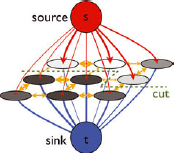
Fig. 14. A cut in a graph. The non-terminal nodes corresponding to each pixel are represented by gray circles. After Reference Boykov and KolmogorovBoykov and Kolmogorov (2004).
Let us define the binary variable Lp
(C) associated to each non-terminal node p as Lp
(C) = 1 if ![]() , 0 else. Denoting ωsp
= P
1 (p), ωpt
= P
0(p) and ωpq
= Vpq
, we have
, 0 else. Denoting ωsp
= P
1 (p), ωpt
= P
0(p) and ωpq
= Vpq
, we have
where ![]() is the indicator function. Thus, a cut in a graph can be directly associated to a binary energy function composed of a local term (P
0, P
1) and a pair interaction potential V. Finding the minimum cut, i.e. the cut with the minimum cost among all cuts, is therefore equivalent to finding the associated energy minimum.
is the indicator function. Thus, a cut in a graph can be directly associated to a binary energy function composed of a local term (P
0, P
1) and a pair interaction potential V. Finding the minimum cut, i.e. the cut with the minimum cost among all cuts, is therefore equivalent to finding the associated energy minimum.
Measurement of binary object surface area with graphs
According to Eqn (A2), the segmentation energy associated to the local intensity model can be directly translated into the graph by correctly setting the edge weights with the terminal nodes. Translating the surface area in terms of edge weight is more complex and requires the capability to relate lengths to the pair interaction potential Vpq . Reference Boykov and KolmogorovBoykov and Kolmogorov (2003) first formalized the link between graph cut and length calculation using the Cauchy–Crofton formula. In 2-D, the Cauchy–Crofton formula relates the Euclidean length of a curve |C| ε to the number nc of intersects with all straight lines in R2:
with ![]() a proper ‘measure’ of the lines subset. This formula can be discretized to provide an approximate length measurement. For example, in Figure 15, only four types of lines directed by a certain neighborhood system are considered: vertical, horizontal and ±45° diagonal lines. The contour of the segmented object intersects one of these lines when it disconnects two nodes linked by these lines. The edge weight associated to each of these lines can thus be set according to the discretized version of the Cauchy– Crofton formula that uses the Voronoi segmentation of the unit sphere (Reference Dañek, Matula, Debled-Rennesson, Domenjoud, Kerautret and EvenDañek and Matula, 2011a,Reference Dañek, Matula, Richard and Brazb). In Figure 15, the edge weights associated to a 2-D example neighborhood system are shown. The neighborhood system used in this work on 3-D images is composed of the 26 first neighbors. Note that computing lengths via the graph-cut approach is consistent with the voxel projection approach (Reference Flin, Furukawa, Sazaki, Uchida and WatanabeFlin and others, 2011) and that it provides a very fast (~2 min for a 10003 voxels image on a PC (4 × 2.7GHz and 6Gb RAM)) and accurate way to compute the surface area of a binary object (Reference Liu, Yi, Zhang, Zheng and PaulLiu and others, 2010; Reference Lehmann and LeglandLehmann and Legland, 2012).
a proper ‘measure’ of the lines subset. This formula can be discretized to provide an approximate length measurement. For example, in Figure 15, only four types of lines directed by a certain neighborhood system are considered: vertical, horizontal and ±45° diagonal lines. The contour of the segmented object intersects one of these lines when it disconnects two nodes linked by these lines. The edge weight associated to each of these lines can thus be set according to the discretized version of the Cauchy– Crofton formula that uses the Voronoi segmentation of the unit sphere (Reference Dañek, Matula, Debled-Rennesson, Domenjoud, Kerautret and EvenDañek and Matula, 2011a,Reference Dañek, Matula, Richard and Brazb). In Figure 15, the edge weights associated to a 2-D example neighborhood system are shown. The neighborhood system used in this work on 3-D images is composed of the 26 first neighbors. Note that computing lengths via the graph-cut approach is consistent with the voxel projection approach (Reference Flin, Furukawa, Sazaki, Uchida and WatanabeFlin and others, 2011) and that it provides a very fast (~2 min for a 10003 voxels image on a PC (4 × 2.7GHz and 6Gb RAM)) and accurate way to compute the surface area of a binary object (Reference Liu, Yi, Zhang, Zheng and PaulLiu and others, 2010; Reference Lehmann and LeglandLehmann and Legland, 2012).
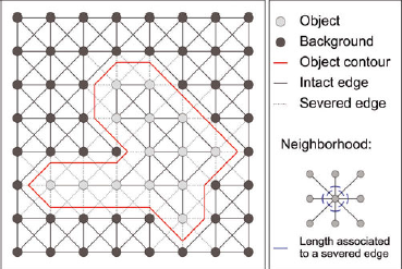
Fig. 15. Graph-cut method to compute a length (2-D case).
Minimization algorithm
Finding the minimal cut can be solved by finding a maximum flow from the source to the sink, which is a problem solvable in polynomial time (Reference Ford and FulkersonFord and Fulkerson, 1956). This proposition is called the ‘min-cut/max-flow’ theorem (Reference Ford and FulkersonFord and Fulkerson, 1956). The maximum flow between s and t can be imagined as the maximum flood of water that goes through the graph using the edges as pipes with a limited capacity (the weights). Finding the maximum flow of water is equivalent to finding the ‘limiting pipes’ .
There exist several polynomial algorithms to solve the min-cut/max-flow problem. The main limitation of these algorithms is the memory usage. Currently, the initial image resulting from a microtomographic scan is very large (>10003 voxels). The corresponding graph is composed of n = 10003 +2 nodes and about 13n edges, and requires >200Gb of memory with usual min-cut/max-flow algorithms (BK2.2; Reference Boykov and KolmogorovBoykov and Kolmogorov, 2004). This amount of RAM is not available on a PC. The exact optimal segmentation on such a huge image is therefore not easily computable. The scalable graph-cut algorithm developed by Reference Delong and BoykovDelong and Boykov (2008) uses the grid structure of the graph to optimize the memory usage. We use an adapted version of their algorithm (freely available for research purposes at http://vision.csd.uwo.ca/code/) that enables the segmentation of massive grids up to 4003 voxels on a PC (6 Gb RAM). This is still not large enough to compute a global optimum on the whole image. However, segmentation is a regional process with relatively small boundary effects. The initial image was thus divided into small overlapping sub-volumes on which the segmentation algorithm is applied.