


1. Introduction
The mechanism of how water surface waves are generated by wind forcing has been a research topic of interest for decades. As early as 1956, Ursell (Reference Ursell1956) pointed out that
‘Wind blowing over a water surface generates waves in the water by a physical process which cannot be regarded as known $\ldots$ The real problem is then how to find the proper simplifications $\ldots$ The present state of our knowledge is profoundly unsatisfactory’.
Many theoretical, numerical and experimental studies on the dynamics of wind-wave generation have been conducted over the past several decades. However, a full understanding of the wind-wave-generation mechanism has not been obtained, including in the initial stages of wave development. Owing to the randomness and smallness of surface waves in the initial response to turbulent air motions, it was challenging to obtain fine-resolution data until the recent growth in computer power and advances in experiment techniques, which motivated systematic investigations and quantitative evaluations of classical early-stage wave generation models.
Several theories have been proposed to explain the fundamental mechanism of wind-wave generation. Jeffreys (Reference Jeffreys1925, Reference Jeffreys1926) first proposed a separation sheltering theory to explain wave growth, which assumes that wind generates separated flows over a wave crest to induce a pressure difference between the windward and leeward sides of the wave and leads to wind input to the wave. However, Jeffreys’ theory overestimates the air–water momentum exchange (Stanton, Marshall & Houghton Reference Stanton, Marshall and Houghton1932). Approximately thirty years later, two seminal theories were separately proposed by Miles (Reference Miles1957) and Phillips (Reference Phillips1957) on wind-wave generation. Miles (Reference Miles1957) assumed that the growth of a surface wave is caused by an instability mechanism of the coupled air–water system and proposed a quasi-linear theory, which predicts that the wave grows exponentially over time owing to the shear instability associated with the critical layer where the speed of wind matches the phase velocity of the wave. Phillips (Reference Phillips1957) argued that the convection of air turbulence pressure fluctuations at the water surface is responsible for early-stage wave generation and proposed a stochastic model, which predicts that the mean square of surface elevations, i.e. surface elevation variance, grows linearly with time. These two pioneering works became cornerstones for the study of wind-wave generation and inspired many follow-up works.
Miles (Reference Miles1957) assumed that there exists an initially prescribed monochromatic wave with small steepness and applied the Rayleigh equation to a two-dimensional mean airflow. He found that the energy transfer rate from the wind to the wave is proportional to the curvature of the mean velocity profile at the critical layer. Later, Miles (Reference Miles1959) further considered the complete Orr–Sommerfeld equation with viscous terms included and found that the viscous effect on wave growth is insignificant. Laboratory experiments (e.g. Shemdin & Hsu Reference Shemdin and Hsu1967; Wilson et al. Reference Wilson, Banner, Flower, Michael and Wilson1973; Larson & Wright Reference Larson and Wright1975) and ocean field observations (e.g. Dobson Reference Dobson1971; Hristov, Miller & Friehe Reference Hristov, Miller and Friehe2003; Grare, Lenain & Melville Reference Grare, Lenain and Melville2013a) qualitatively confirmed Miles’ critical-layer theory (Miles Reference Miles1957, Reference Miles1959), but discrepancies in the wave-growth rate remain between the theory and measurements. The effects of wave-induced turbulence stress in the air boundary layer were further considered to extend the Miles theory (e.g. Townsend Reference Townsend1972; Jacobs Reference Jacobs1987; Van Duin & Janssen Reference Van Duin and Janssen1992; Miles Reference Miles1993). Belcher & Hunt (Reference Belcher and Hunt1993) applied the rapid distortion theory to a four-layer asymptotic boundary layer structure above a slow-moving wave and proposed the non-separated sheltering theory to explain the origin of the phase difference between the wave and the pressure perturbation and the formation of the pressure-induced form drag. Following the above theoretical developments, wave-induced turbulence structures have been extensively studied numerically (e.g. Sullivan, McWilliams & Moeng Reference Sullivan, McWilliams and Moeng2000; Kihara et al. Reference Kihara, Hanazaki, Mizuya and Ueda2007; Yang & Shen Reference Yang and Shen2010; Hao & Shen Reference Hao and Shen2019) and experimentally (e.g. Hsu, Hsu & Street Reference Hsu, Hsu and Street1981; Grare et al. Reference Grare, Peirson, Branger, Walker, Giovanangeli and Makin2013b; Grare, Lenain & Melville Reference Grare, Lenain and Melville2018).
Unlike the Miles theory, in which the water wave is initially prescribed, the Phillips theory focuses on how waves are generated from an initially flat water surface (Phillips Reference Phillips1957). Phillips conjectured that the convection of air pressure fluctuations plays an essential role in the early stage of wind-wave generation. In this theory, the resonance between waves and air pressure fluctuations leads to initial wave development, resulting in a quadratic growth of the surface elevation variance at certain wavenumbers satisfying the resonance condition. This duration is referred to as the initial stage by Phillips (Reference Phillips1957). After the time far exceeds the development time of pressure fluctuations (see Phillips Reference Phillips1957, p. 421), the surface elevation variance grows linearly with time. This stage is referred to as the principal stage (Phillips Reference Phillips1957). The Phillips theory is based on Taylor's frozen hypothesis (Taylor Reference Taylor1938), which assumes that turbulent fluctuations are convected at a certain velocity by the mean flow. Although the original frozen hypothesis only focuses on turbulent velocity fluctuations, the convection of wall pressure fluctuations is also validated through experiments (e.g. Farabee & Casarella Reference Farabee and Casarella1991; Abraham & Keith Reference Abraham and Keith1998) and numerical simulations (e.g. Choi & Moin Reference Choi and Moin1990; Hu, Morfey & Sandham Reference Hu, Morfey and Sandham2006). Based on the linearised water wave equation, Phillips (Reference Phillips1957) derived a stochastic second-order ordinary differential equation for each wave elevation component in Fourier space. The long-term asymptotic solution predicts that the mean square of wave elevations grows linearly with the elapsed time  $t$, and the expression is
 \begin{equation} \langle \eta^{2} \rangle\sim \frac{\langle{p^{2}}\rangle t}{2\sqrt{2}\rho^{w2}U_{p} g},\end{equation}
where  $\eta$ is the wave surface elevation, $p$ is turbulence pressure fluctuations of airflow at the water surface, $\rho ^{w}$ is the water density, $U_{p}$ is the convection velocity of pressure fluctuations, $g$ is the gravitational acceleration and $\langle \cdot \rangle$ denotes the spatial averaging operator. It should be noted that (1.1) is not a quantitative prediction of the surface elevation variance because Phillips used ‘a rough approximation’ to relate the integral time scale of pressure fluctuations to the convection velocity (see Phillips Reference Phillips1957, p. 437). Phillips (Reference Phillips1957) assumed that the prefactor in (1.1) is $1$ and conducted comparisons with observations of wave fields (see Phillips Reference Phillips1957, § 4.3). The right-hand side of (1.1) is referred to as the Phillips model for predicting the surface elevation variance in the principal stage, which has been widely used as a quantitative prediction of wave growth based on the Phillips theory (see e.g. Snyder & Cox Reference Snyder and Cox1966; Barnett & Wilkerson Reference Barnett and Wilkerson1967; Longuet-Higgins Reference Longuet-Higgins1969; Lin et al. Reference Lin, Moeng, Tsai, Sullivan and Belcher2008; Paquier, Moisy & Rabaud Reference Paquier, Moisy and Rabaud2016; Perrard et al. Reference Perrard, Lozano-Durán, Rabaud, Benzaquen and Moisy2019). Lin et al. (Reference Lin, Moeng, Tsai, Sullivan and Belcher2008) conducted direct numerical simulation (DNS) of wave generation underneath a turbulent airflow and first captured the linear-growth rate in the principal stage of the wave generation process. The authors compared their DNS result of $\langle \eta ^{2}\rangle$ with the right-hand side of (1.1) and found that they are of the same order of magnitude.
The intensity of turbulent pressure fluctuations exerted on the water surface is usually low, and thus, the Phillips theory is commonly believed to dominate wave evolution only in the early development of wind waves. The quantification of small-amplitude wave heights in experiments requires highly accurate instruments and can be complicated by environmental noise. The direct measurement of pressure at the wave surface is challenging, and the surface value of pressure is usually obtained by extrapolation (see Peirson, Garcia & Pells Reference Peirson, Garcia and Pells2003). Kawai (Reference Kawai1979) studied the initial wave patterns under wind forcing in a wave tank but did not observe the linear growth of surface elevation variance. Kahma & Donelan (Reference Kahma and Donelan1988) discussed the possible relations between experimentally observed initial excitations of water waves at low wind speed and the resonance mechanism in the Phillips theory. Recently, Zavadsky & Shemer (Reference Zavadsky and Shemer2017) first directly observed the linear growth of surface elevation variance in the principal stage in a high-resolution laboratory experiment, which partially supported the Phillips theory. However, the pressure fluctuations on the water surface cannot be accurately measured, which poses challenges for a quantitative validation between the experimental data and the theory.
The theories of Phillips (Reference Phillips1957) and Miles (Reference Miles1957) are based on two different wave generation mechanisms. Miles (Reference Miles1960) combined these two mechanisms and pointed out that the linear growth of surface elevation variance occurs in early wind-wave development, while the exponential growth occurs in the late phase. However, a strict classification of different wave growth stages has not yet been obtained. Lin et al. (Reference Lin, Moeng, Tsai, Sullivan and Belcher2008) observed the linear-growth stage and the exponential growth stage of waves in a DNS study. Zavadsky & Shemer (Reference Zavadsky and Shemer2017) reported laboratory observations of the linear-growth stage. Before the linear-growth stage, however, they also measured a period in which the wave grows exponentially over time, which is not predicted by the Phillips theory. Zonta, Soldati & Onorato (Reference Zonta, Soldati and Onorato2015) numerically studied wave generation in a countercurrent air–water turbulent flow and showed that the wave amplitude grows in time following a power law,  $\eta \propto t^{2/5}$. Paquier, Moisy & Rabaud (Reference Paquier, Moisy and Rabaud2015) experimentally studied the viscous effect of wind-wave generation by controlling the kinematic viscosity of the mixture of water and glycerol and showed that viscosity plays an important role in the formation of small water wrinkles. Based on the experimental work of Paquier et al. (Reference Paquier, Moisy and Rabaud2015, Reference Paquier, Moisy and Rabaud2016), Perrard et al. (Reference Perrard, Lozano-Durán, Rabaud, Benzaquen and Moisy2019) proposed a spectral theory for the spatial-temporal evolution of wrinkles under low wind conditions. Nové-Josserand et al. (Reference Nové-Josserand, Perrard, Lozano-Durán, Benzaquen, Rabaud and Moisy2020) numerically studied the effect of a weak current on wind-generated waves in the wrinkle regime. Recently, Wu & Deike (Reference Wu and Deike2021) numerically investigated the growth rate of gravity–capillary waves in the viscous regime. Comparisons between wave evolution in a wave-tank and numerical model were conducted by Shemer, Singh & Chernyshova (Reference Shemer, Singh and Chernyshova2020) and Shemer & Singh (Reference Shemer and Singh2021). We note that the linear wave theory is adequate to describe the wave dynamics in the early development of water waves when the wave amplitude is small. However, as the wave amplitude grows over time, the importance of wave nonlinearity increases. Resonant interactions can occur among a group of wave components for the wave energy of different wave components to exchange, such as the four-wave resonant interaction in deep water waves (see Hasselmann Reference Hasselmann1962, Reference Hasselmann1963).
Numerical simulations can provide detailed descriptions of the flow field, such as the structures of turbulent pressure, shear stress and velocity fluctuations, and have become a powerful tool for studying wind–wave interactions with the increasing capability of computing power. Large-eddy simulation (LES) and DNS are common simulation methods used in recent years to study the interactions between waves and turbulence. LES computes the turbulent motions down to grid-sized scales and uses subgrid-scale models to capture smaller-scale effects. Sullivan et al. (Reference Sullivan, Edson, Hristov and McWilliams2008), Sullivan, McWilliams & Patton (Reference Sullivan, McWilliams and Patton2014), Hara & Sullivan (Reference Hara and Sullivan2015), Sullivan et al. (Reference Sullivan, Banner, Morison and Peirson2018), Zhang, Huang & Xu (Reference Zhang, Huang and Xu2019), Hao & Shen (Reference Hao and Shen2019), Åkervik & Vartdal (Reference Åkervik and Vartdal2019), Cao, Deng & Shen (Reference Cao, Deng and Shen2020) and Cao & Shen (Reference Cao and Shen2021) performed LES over different wave surfaces. DNS simulates Navier–Stokes equations directly and can resolve detailed turbulence structures at the cost of fine grid resolutions. Sullivan et al. (Reference Sullivan, McWilliams and Moeng2000), Kihara et al. (Reference Kihara, Hanazaki, Mizuya and Ueda2007), Yang & Shen (Reference Yang and Shen2010, Reference Yang and Shen2017) and Druzhinin, Troitskaya & Zilitinkevich (Reference Druzhinin, Troitskaya and Zilitinkevich2012) performed DNS of turbulent airflow over prescribed monochromatic wave boundary. Coupled air–water simulations have also been performed, usually focusing on the dynamics of irregular waves or scalar transfer (e.g. Lin et al. Reference Lin, Moeng, Tsai, Sullivan and Belcher2008; Liu et al. Reference Liu, Kermani, Shen and Yue2009; Komori et al. Reference Komori, Kurose, Iwano, Ukai and Suzuki2010; Zonta et al. Reference Zonta, Soldati and Onorato2015; Kurose et al. Reference Kurose, Takagaki, Kimura and Komori2016; Campbell, Hendrickson & Liu Reference Campbell, Hendrickson and Liu2016). Compared with LES, the Reynolds number in DNS is relatively low when resolving the Kolmogorov scale (Moin & Mahesh Reference Moin and Mahesh1998). For the study of the fundamental physical mechanisms of wind-wave generation occurring at small scales, DNS is a suitable research tool.
The present study focuses on the principal stage in the Phillips theory. Using the computational framework developed by Yang & Shen (Reference Yang and Shen2011a,Reference Yang and Shenb) and Xuan & Shen (Reference Xuan and Shen2019), we conduct high-resolution DNS for turbulent airflow-induced wave growth starting with a flat water surface. From the DNS results, we rigorously evaluate the Phillips theory in the principal stage, show convincing numerical evidence on its existence, and perform comprehensive analyses on the statistics of waves forced by wind. We further develop a new random sweeping turbulence pressure–wave interaction model to quantitatively predict the wave-growth rate in the principal stage, which shows substantial improvement over the estimation by the Phillips model. The remainder of the paper is organised as follows. In § 2, we introduce the problem set-up and simulation method. In § 3, we describe the multiple stages of wind-wave generation in the DNS results. In § 4, we present a theoretical framework of the closure model for wave generation in the principal stage and derive an asymptotic solution of surface elevation variance. In § 5, we evaluate our theoretical model with the DNS results. Conclusions are given in § 6.
2. Problem set-up and simulation cases
2.1. Problem set-up
Following Lin et al. (Reference Lin, Moeng, Tsai, Sullivan and Belcher2008), we consider the canonical problem of a turbulent air Couette flow over an initially flat water surface. The simulations are conducted in a horizontally periodic rectangular domain, as shown in figure 1. To obtain the airflow with fully developed turbulence as the initial condition, we perform a DNS for a turbulent air shear-driven flow and keep the air–water interface flat and the water calm. Constant shear stress is applied on the top of the air domain in the  $x$-direction to drive the airflow. After the turbulent airflow has reached a statistically steady state, we release the constraint of the water surface and let the entire air–water system evolve dynamically. The water surface deforms owing to the forcing by the turbulent motions of air to form waves. Details of the computational cases are given in the following sections.

Figure 1. Configuration of the simulation set-up and sketch of the initial condition of shear-driven turbulent airflow over an initially calm water surface.
2.2. Governing equations and boundary conditions
2.2.1. Governing equations
We simulate the motions of air and water and focus on their hydrodynamic properties. Air and water motions are governed by incompressible Navier–Stokes equations. The entire physical space can be split into a water domain and air domain, with their adjacent boundary being the dynamically evolving air–water interface.
Cartesian coordinates  $(x^{a}, y^{a}, z^{a})$ and $(x^{w}, y^{w}, z^{w})$ are established in the air and water domains, with the superscripts ‘ $a$’ and ‘ $w$’ representing the air and water domains, respectively. When the superscript is not explicitly specified, the variables are for both the air and the water domains. The coordinates are established such that the $(x,y)$ plane is horizontal and the $z$-axis denotes the vertical direction pointing upwards. The two coordinates in the air and water domains are coincident with each other, and their origins $(x, y, z)=(0,0,0)$ are located on the plane of the mean water surface level. The incompressible continuity and Navier–Stokes equations are
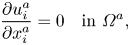 $$\begin{gather} \frac{\partial u^{a}_i}{\partial x_i^{a}}=0 \quad \text{in }\varOmega^{a}, \end{gather}$$
 $$\begin{gather}\frac{\partial u^{a}_i}{\partial t}+\frac{\partial (u^{a}_i u^{a}_j)}{\partial x_j^{a}} ={-}\frac{1}{\rho^{a}}\frac{\partial p^{a}}{\partial x_i^{a}}+\nu^{a} \frac{\partial^{2} u^{a}_i}{\partial x_j^{a}\partial x_j^{a}} \quad \text{in } \varOmega^{a}, \end{gather}$$
 $$\begin{gather}\frac{\partial u^{w}_i}{\partial x_i^{w}}=0 \quad \text{in }\varOmega^{w}, \end{gather}$$
 $$\begin{gather}\frac{\partial u^{w}_i}{\partial t}+\frac{\partial (u^{w}_i u^{w}_j)}{\partial x_j^{w}} ={-}\frac{1}{\rho^{w}}\frac{\partial p^{w}}{\partial x_i^{w}}+\nu^{w} \frac{\partial^{2} u^{w}_i}{\partial x_j^{w}x_j^{w}}\quad \text{in }\varOmega^{w}. \end{gather}$$
Here,  $u_i(i=1,2,3)=(u,v,w)$ are the velocity components in Cartesian coordinates, $p$ denotes the pressure and $\nu$ is the kinematic viscosity. The horizontal domain size for both the air and water is $L_x\times L_y$. The heights of the air domain $H^{a}$ and water domain $H^{w}$ are defined as the distance from the mean level of the air–water interface to the upper and lower boundaries, respectively, and we set $H^{a}=H^{w}=H$ in this study. The deviation of the local water surface height from its mean level is denoted as $\eta (x,y,t)$. Equations (2.1a) and (2.1b) are defined in the air domain $\varOmega ^{a}=\{(x,y,z) \mid 0\leq x\leq L_x,0\leq y\leq L_y,\eta (x,y,t)\leq z\leq H\}$, and (2.1c) and (2.1d) are defined in the water domain $\varOmega ^{w}=\{(x,y,z) \mid 0\leq x\leq L_x,0\leq y\leq L_y,-H\leq z\leq \eta (x,y,t)\}$. The closures of $\varOmega ^{a}$ and $\varOmega ^{w}$ are time varying.
To accurately resolve the turbulence fluctuations near the air–water interface and explicitly capture the deformation of the interface, we perform the DNS on a curved grid that fits the dynamically evolving water surface (Yang & Shen Reference Yang and Shen2011a,Reference Yang and Shenb; Xuan & Shen Reference Xuan and Shen2019). The flow solvers have been used and validated extensively in previous studies (Yang & Shen Reference Yang and Shen2010; Yang, Meneveau & Shen Reference Yang, Meneveau and Shen2013, Reference Yang, Meneveau and Shen2014a,Reference Yang, Meneveau and Shenb; Hao & Shen Reference Hao and Shen2019; Xuan & Shen Reference Xuan and Shen2019; Cao et al. Reference Cao, Deng and Shen2020; Xuan, Deng & Shen Reference Xuan, Deng and Shen2020; Cao & Shen Reference Cao and Shen2021). In the present study, the air and water domains are discretised on a wave-surface-fitted curvilinear grid. The discrete incompressible Navier–Stokes equations are solved in the air and water domains synchronically and coupled through boundary conditions on the air–water interface at each timestep to enforce the matching of velocity and stresses between air and water. The time evolution of the air–water interface is calculated through the nonlinear kinematic boundary conditions of the interface. Details of the numerical schemes are provided in Appendix A.
2.3. Simulation cases
We first generate a fully developed turbulent airflow while keeping the water calm, i.e. enforcing the air–water interface as a no-slip boundary when performing the air-side simulation only. At the beginning of the simulation, we initialise the airflow velocity field by adding random divergence-free velocity fluctuations to a mean profile, which contains the viscous sublayer and the logarithmic inner layer following the law of the wall on both the bottom and top boundaries. The total simulation time for shear-driven turbulence development is approximately  $6.7\times 10^{5}$ viscous time units, normalised by the air friction velocity and kinematic viscosity, before the coupled air–water simulation starts. Validation of DNS of the turbulent airflow is discussed in § 1 of the supplementary materials are available at https://doi.org/10.1017/jfm.2021.1153. After the turbulent airflow reaches a statistically steady state, we conduct the simulation for the coupled air and water motions with the interface evolving dynamically.
We use the densities of air and water at sea level and the temperature of  $15\,^{\circ }$C, which are $\rho ^{a}={1.225}\ \mathrm {kg\ m}^{-3}$ and $\rho ^{w}={9.99\times 10^{2}}\ \mathrm {kg\ m}^{-3}$, respectively, and the air–water density ratio is $\rho ^{a}/\rho ^{w}=1.23\times 10^{-3}$. The kinematic viscosities of water and air are $\nu ^{a}={1.46\times 10^{-5}}\ \mathrm {m\ s}^{-2}$ and $\nu ^{w}={1.14\times 10^{-6}}\ \mathrm {m\ s}^{-2}$, respectively. The corresponding water–air kinematic viscosity ratio is $\nu ^{a}/\nu ^{w}=12.8$. The Reynolds number is limited in the DNS. Note that the computational cost for the present simulation on a boundary-fitted moving grid is substantially higher than that for regular domains. The Reynolds numbers based on the friction velocity $u_\tau$ and each domain height $H$ are $Re_\tau ^{a}={u_\tau ^{a} H^{a}}/{\nu ^{a}}=268$ and $Re_\tau ^{w}={u_\tau ^{w}H^{w}}/{\nu ^{w}}=120$ for air and water, respectively. The relation between $Re_\tau ^{a}$ and $Re_\tau ^{w}$ is (see Liu et al. Reference Liu, Kermani, Shen and Yue2009)
 \begin{equation} {Re}_\tau^{a}=\sqrt{\frac{\rho^{w}}{\rho^{a}}}\frac{\nu^{w}}{\nu^{a}}{Re}_\tau^{w}. \end{equation}
The friction velocity  $u_\tau$ is defined as $u_\tau =\sqrt {\tau _s/\rho }$, where $\tau _s$ denotes the mean shear stress exerted on the top or bottom boundary. In the present simulations, the air friction velocity is $u_\tau ^{a}={0.08}\ \mathrm {m\ s}^{-1}$, which is comparable to the previous DNS studies of air–water interactions (Lin et al. Reference Lin, Moeng, Tsai, Sullivan and Belcher2008; Zonta et al. Reference Zonta, Soldati and Onorato2015), and the corresponding characteristic length scale is $H={0.0489}\ \mathrm {m}$. The simulation domain sizes are $(2{\rm \pi} H,{\rm \pi} H,H)$ for both air and water. Based on the gravitational acceleration $g={9.81}\ \mathrm {m\ s}^{-2}$, surface tension of the air–water interface $\sigma ={7.35\times 10^{-2}}\ \mathrm {N\ m}^{-1}$, and the mean velocity of the air at the upper boundary $U^{a}=31u_\tau ^{a}$, we can obtain the Froude number ${Fr^{a}}=U^{a}/\sqrt {gH^{a}}=3.58$ and Weber number ${We^{a}}=\rho ^{w}U^{a2}H^{a}/\sigma =4088$. The parameters of the simulation cases are summarised in table 1. The capillary length scale is $l_c=\sqrt {\sigma /(\rho ^{w}g)}=Fr^{a}/\sqrt {We^{a}}H=0.056H$. The domain sizes relative to the capillary length scale are $L_x=112.2l_c$ and $L_y=56.1 l_c$ in $x$- and $y$-directions, respectively.
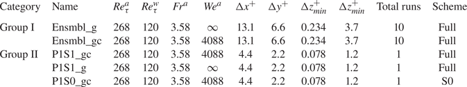
Table 1. Summary of simulation case parameters. The abbreviations ‘g’ and ‘gc’ denote gravity waves and gravity–capillary waves, respectively, and the superscript ‘ $+$’ denotes normalisation by the viscous length scale $\nu ^{a}/u_\tau ^{a}$ in the air domain. The column named ‘Scheme’ lists the air–water coupling schemes. ‘Full’ denotes the fully coupled air–water interface scheme where the transfer of both the turbulence pressure and shear stress from the air to the water surface is applied. ‘S0’ denotes the case where the transfer of turbulent air shear stress on the air–water interface to the water domain is turned off.
The non-dimensional timestep  $\Delta t$ based on the velocity at the mean top boundary $U^{a}$ and domain height $H^{a}$ is chosen as $\Delta tU^{a}/H^{a}=9\times 10^{-4}$, which is constrained by the Courant–Friedrichs–Lewy condition. The generation of surface waves is an unsteady problem, and the initial condition of the turbulent airflow field may bring uncertainties to the long-term behaviour of wave growth. We conduct multiple ensemble simulations to reduce the effects of the selected turbulent field when the surface starts to deform. Specifically, based on the computer resource availability, we perform ten independent simulations, denoted by Group I, with a $128\times 128\times 128$ grid in both the air and water domains. Moreover, we perform superresolution simulations, denoted by Group II, using the same physical parameters with a $384\times 384\times 384$ grid in both the air and water domains. In both Group I and Group II, we conduct different simulations with the same initial conditions for gravity–capillary waves and gravity waves. The grid resolutions in the viscous length scale are $(\Delta x^{+},\Delta y^{+},\Delta z_{min}^{+})=(13.1,6.6,0.234)$ and $(\Delta x^{+},\Delta y^{+},\Delta z_{min}^{+})=(4.4,2.2,0.078)$ for Group I and Group II simulations, respectively. Here, the superscript ‘ $+$’ denotes the normalisation based on the viscous length scale $\nu ^{a}/u_\tau ^{a}$, $\Delta x^{+}$ and $\Delta y^{+}$ denote the grid space in the horizontal directions and $\Delta z_{min}^{+}$ denotes the minimum grid space near the air–water interface in the vertical direction. All grid resolutions are sufficient for the DNS study (Moin & Mahesh Reference Moin and Mahesh1998). The grid resolutions compared with the capillary length scale are $(\Delta x/l_c, \Delta y/l_c)= (0.877,0.438)$ in Group I simulations and $(\Delta x/l_c, \Delta y/l_c)= (0.292,0.146)$ in Group II simulations. The corresponding wavelength (i.e. $2{\rm \pi} l_c$) in the $x$-direction is resolved by 7 grid points and 21 grid points in Group I and Group II simulations, respectively. The present grid resolutions in the capillary length scale are adequate for simulating gravity–capillary waves and are comparable to other free-surface simulations in the literature (e.g. Lin et al. Reference Lin, Moeng, Tsai, Sullivan and Belcher2008; Deike, Pizzo & Melville Reference Deike, Pizzo and Melville2017; Yu et al. Reference Yu, Hendrickson, Campbell and Yue2019). We note that higher resolution is needed to fully resolve parasitic capillary waves that occur at the leeward side of steep waves (Deike, Popinet & Melville Reference Deike, Popinet and Melville2015), which is not present in our study because our work only involves the early stage of wind-wave generation when the wave steepness is small. We also note that because coupled air and water simulations are performed and a surface-fitted curvilinear grid is employed, the computational cost is high (Yang & Shen Reference Yang and Shen2011b; Xuan & Shen Reference Xuan and Shen2019). On the massively parallel Onyx supercomputer at the U.S. Army Engineer Research and Development Center, which is a Cray 40/50 system using 2.8 GHz Intel Xeon E5-2699v4 Broadwell processors, simulations take approximately $3.4\times 10^{5}$ CPU hours for each case in Group I and $7.0\times 10^{6}$ CPU hours for each case in Group II. The total computational cost is estimated $2.8\times 10^{7}$ CPU hours. In the simulations, the airflow is strong enough to generate surface waves. To illustrate the relative velocity differences between air turbulent fluctuations and water waves, we plot the wavenumber–phase velocity spectrum of air pressure fluctuations at the water surface $S(k_x, c)=\langle \tilde \varPi _p\rangle _y (k_x,\omega =ck_x)$ in figure 2, where $\langle \tilde \varPi _p\rangle _y$ is the spanwise-averaged wavenumber–frequency spectrum of the air pressure fluctuations along the streamwise direction, $k_x$ is the streamwise wavenumber, $\omega$ is the frequency and $c=\omega k_x^{-1}$ is the phase velocity. We use a wave surface-fitted grid to conduct DNS, and the air pressure at the water surface $p(x,y)=p^{a} (x,y,\eta (x,y,t))$ can be explicitly calculated. This approach is consistent with the Zakharov formulation (Zakharov Reference Zakharov1968). The air pressure at the water surface is expressed as a function of $x$ and $y$. The averaging and norm calculations are computed via integral on the boundary-fitted grid $(x,y,\eta (x,y,t))$ which corresponds to the water surface. We sample $34\ 488$ consecutive instantaneous snapshots to calculate the spectrum in the early duration of $20H/u_\tau ^{a}$ when the wave amplitudes are not significant enough to modulate the airflow. The black line in figure 2 represents the averaged convection velocity of pressure fluctuations, which is computed by (see Del Álamo & Jiménez Reference Del Álamo and Jiménez2009)
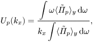 \begin{equation} U_{p}(k_x)=\frac{\displaystyle\int \omega \langle\tilde\varPi_p\rangle_y \, {{\rm d}} \omega}{\displaystyle k_x\int \langle\tilde\varPi_p\rangle_y\, {{\rm d}} \omega}, \end{equation}
and decays slightly as the wavenumber  $k_x$ increases, indicating that the larger scales of turbulent pressure fluctuations are convected faster (Kim Reference Kim1989). In figure 2, the phase velocities of gravity–capillary waves $c_{gc}(k_x)$ and gravity waves $c_{g}(k_x)$ are respectively calculated as
 $$\begin{gather} c_{gc}(k_x)=\sqrt{\frac{1}{{Fr}^{2}}\frac{1}{|k_x|}+\frac{1}{{We}}|k_x|}, \end{gather}$$
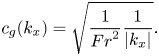 $$\begin{gather}c_{g}(k_x)=\sqrt{\frac{1}{{Fr}^{2}}\frac{1}{|k_x|}}. \end{gather}$$
The phase speed of gravity waves decreases monotonically as the wavenumber increases. For gravity–capillary waves, the phase velocity has a global minimum at  $k_{{crit}}H=\sqrt {{We}}/{Fr}=17.9$. When the wavenumber is larger than the critical wavenumber, $c_{gc}(k_x)$ increases with $|k_x|$. One can expect that at sufficiently high wavenumbers, $c_{gc}(k_x)$ is larger than the convection velocity of pressure fluctuations $U_{p}(k_x)$. However, the spectrum $\tilde \varPi _p$ decays fast with wavenumber $k_x$ for large $|k_x|$ so that its contribution to wave growth is negligible. In the present study, the phase velocities of both gravity–capillary waves and gravity waves are less than the resolved pressure convection velocity (figure 2). This result is consistent with the assumption of the Phillips theory that the pressure convection velocity is much larger than the wave phase velocity, which makes our DNS suitable for evaluating the Phillips theory.
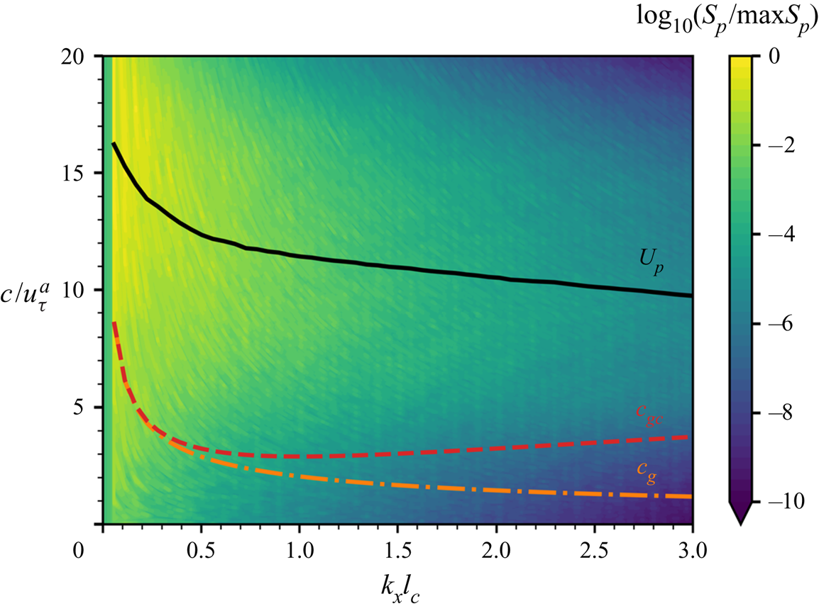
Figure 2. The wavenumber–phase velocity spectrum of air pressure fluctuations  $S_p(k_x,c)$ at the water surface, normalised by its maximum value. The black line (——) is the averaged convection velocity of pressure fluctuations at the water surface, $U_{p}(k_x)$. The red (– –) and orange (– $\cdot$ –) curves represent the phase velocities of gravity–capillary waves and gravity waves, $c_{gc}(k_x)$ and $c_g(k_x)$, respectively. The result shows that the air pressure convection velocity is larger than the wave phase velocity for all wavenumbers.
2.4. Descriptions of datasets
After the coupled simulations start and the surface begins to deform due to air motions, surface variables such as elevations and air surface pressure are collected for a duration of  $75H/u_\tau ^{a}$, i.e. 75 times the largest eddy turnover time. Surface waves are initially generated from a calm water surface, and simulations stop in the stage when waves grow exponentially with time. During the wave-generation process, snapshots of instantaneous variables are output every $1.44\times 10^{-2}H/u_\tau ^{a}$ for Group I simulations and every $5.8\times 10^{-4}H/u_\tau ^{a}$ for Group II simulations. The higher sampling frequency for Group II is beneficial for conducting analysis in the spectral space.
3. Multiple stages of wind-generated wave development
In this section, we show the multiple stages of wind-generated wave development in our DNS results in §§ 3.1 and 3.2. The effects of air turbulence shear stress on wave growth in the principal stage are discussed in § 3.3. Following § 3, theoretical analyses are performed in § 4, and a comparison with the DNS data is presented in § 5.
3.1. Instantaneous flow field
Figure 3 shows instantaneous snapshots of the air–wave–water field at different times in the superresolution simulation (Group II). The air–water interface is flat at  $t=0$, and the contours of water surface deformation in figure 3(a) illustrate the initial response of the interface to the imposition of air turbulence pressure and shear stress fluctuations. Figures 3(b) and 3(c) show the flow field in the early phase when the turbulent airflow distorts the water surface and generates small-scale irregular waves. Figure 3(d) illustrates a late phase when spanwise dominant waves are generated. In the water domain, wind shear generates a thin shear layer underneath the water surface. We further conduct a spectral analysis of the surface elevation at the four time instants of the superresolution simulation (Group I) shown in figure 3. Table 2 shows the wavenumbers of the five most energetic wave components at the four time instants and their percentages of the total wave energy. At the very beginning when $tu_\tau ^{a}/H=0.03$, the energy fraction of each wave component is very low (less than $3\,\%$), and the five most energetic waves contain only $12.4\,\%$ of the wave energy in total. In the early phase of wave development (see table 2a–c), the spanwise wavenumbers ( $k_y$) of the five most energetic waves are mostly larger than the streamwise wavenumbers ( $k_x$), which results in the streak-like surface wave pattern as shown in figures 3(a)–3(c). In the late phase (table 2d), the spanwise wavenumbers of the most energetic waves become smaller, and the wave components are mostly streamwise dominant (see figure 3d). As the elapsed time increases, the wave energy accumulates at selected wavenumbers. The total of the wave energy percentages of the five most energetic wave components rises from $12.4\,\%$ at $tu_\tau ^{a}/H=0.03$ to $63.8\,\%$ at $tu_\tau ^{a}/H=45.8$.

Figure 3. Snapshots of instantaneous air–water interface deformation and velocity field of air and water at: (a)  $tu_\tau ^{a}/H=0.03$; (b) $tu_\tau ^{a}/H=2.9$; (c) $tu_\tau ^{a}/H=12.2$; (d) $tu_\tau ^{a}/H=45.8$. For all cases, contours on representative vertical planes show the streamwise velocity $u$ in the air and water domains normalised by the friction velocity $u_\tau$. The water surface deformation is plotted on its actual scale, and contours of surface deformation are normalised by the instantaneous maximum absolute value. For clarity, only the near-surface half of the computational domain is plotted.
Table 2. Wavenumber ( $k_xl_c,k_yl_c$) and wave energy percentage ( $\hat \varPsi _{\eta }/\langle \eta ^{2}\rangle$) of the five most energetic wave components at the time instants $tu_\tau ^{a}/H=0.03,2.9,12.2,45.8$ shown in figure 3. Here, $\hat \varPsi _{\eta }$ denotes the wave energy at the wavenumber $(k_x,k_y)$ defined in (4.14). The symbol ‘sum’ represents the summation of wave energy percentages of the five most energetic wave components.

3.2. Temporal behaviour of wave growth
Figure 4 shows the temporal growth of the surface elevation variance and pressure variance for the ensemble simulations of gravity–capillary waves (case Ensembl_gc in Group I) and the superresolution simulation of gravity–capillary waves (case P1S1_gc in Group II). All variables are normalised using the air domain height  $H$ or the capillary length scale $l_c$ and the friction velocity $u_\tau$. Group I has ten independent simulation cases, and we calculate the ensemble average and its $99\,\%$ confidence interval (CI). Plots of individual realisations are visualised in Appendix B. The $99\,\%$ CI is computed as $(\bar {x}-2.58s/\sqrt {n},\bar {x}+2.58s/\sqrt {n})$, where $\bar {x}$, $s$ and $n$ denote the sample mean, standard deviation and number of realisations, respectively. As shown in figure 4, the results from the superresolution group II lie within the 99 % CI region of Group I. The growth of surface elevation variance $\langle \eta ^{2}\rangle$ consists of multiple stages. Here, the bracket $\langle \cdot \rangle$ denotes the spatial average on the horizontal plane. The growth rate is low in the early wind-wave development but rises explosively in the late phase. This phenomenon can be further explicitly demonstrated using log-scale plots. Figure 4(c) uses logarithmic scales in both the $x$- and $y$-axes. A straight line indicates the power law, $\langle \eta ^{2}\rangle \propto t^{\alpha }$, with the index $\alpha$ being a constant. Initially, the index $\alpha =4$ shows a nascent stage when waves first respond to the sudden imposition of turbulent airflow. The index $\alpha$ decreases to 1 shortly, and the corresponding linear growth lasts for a duration of $O(20) H/u_\tau ^{a}$, which corresponds to the principal stage in the Phillips theory (Phillips Reference Phillips1957) that is the focus of this study. More rigorous validations of the linear growth of surface elevation variance in this stage are discussed in Appendix C, where we show that the principal stage lasts until the elapsed time reaches $tu_\tau ^{a}/H\approx 20$. The fast growth rate after the principal stage is exhibited in figure 4(d), with the $x$-axis plotted on a linear scale and the $y$-axis plotted on a logarithmic scale. The straight line when the elapsed time $tu_\tau ^{a}/H>50$ shows the exponential growth of surface elevation variance $\langle \eta ^{2}\rangle$ (Miles Reference Miles1957). A more detailed analysis on the exponential growth behaviours of surface elevation variance in the late stage is discussed in § 2 of the supplementary materials.

Figure 4. The overall temporal growth behaviours of surface elevation variance  $\langle \eta ^{2}\rangle$ and pressure variance $\langle p^{2}\rangle$: (a) $\langle \eta ^{2}\rangle$, linear scale in both the $x$- and $y$-axes; (b) $\langle p^{2}\rangle$, linear scale in both the $x$- and $y$-axes; (c) $\langle \eta ^{2}\rangle$, logarithmic scale in both the $x$- and $y$-axes; (d) $\langle \eta ^{2}\rangle$, linear scale in the $x$-axis and logarithmic scale in the $y$-axis. In (a,c,d), surface elevation variance $\langle \eta ^{2}\rangle$ is normalised by the air domain height $H$ and the capillary length scale $l_c$, shown on the left and right $y$-axes, respectively. The solid blue line denotes the sample average of the 10 realisations of Group I, and the light blue shaded area denotes the $99\,\%$ confidence interval of the ensemble mean. The orange line represents the surface elevation variance for the superresolution simulation (Group II).
In the Phillips theory, the motions of airflow are not affected by surface waves. Waves are generated by the motions of airflow, but the airflow is not affected by the air–water interface deformation because the wave amplitude is very small in the principal stage. The linear growth of surface elevation variance is contributed by the space–time turbulent characteristics of air pressure fluctuations. In the Miles theory, coherent motions of surface waves and air mean flow trigger the instability induced at the critical layer, and the unstable modes have exponential growth in time. However, the Miles theory cannot predict a minimum threshold of wave amplitude for the onset of instability. During the transition period,  $20< tu_\tau ^{a}/H<50$, both these two mechanisms are expected to have influences. As the resonance mechanism of the pressure fluctuations continues contributing to the wave growth, the finite-amplitude surface waves begin to disturb the turbulent airflow, and coherent motions between waves and airflow are formed. The critical-layer instability caused by coherent motions gradually dominates the resonance mechanism, which leads to the exponential growth of the surface elevation variance. Determination of a criterion for the transition between the linear-growth regime (Phillips Reference Phillips1957) and the exponential growth regime (Miles Reference Miles1957) is currently an open research problem. Perrard et al. (Reference Perrard, Lozano-Durán, Rabaud, Benzaquen and Moisy2019) analysed the liquid viscosity scaling of the amplitude of viscous saturated wrinkles using the experimental data from Paquier et al. (Reference Paquier, Moisy and Rabaud2016) and proposed a criterion for the minimum root mean square (r.m.s.) of surface elevation for the exponential growth behaviour, $\eta _{rms}=A\delta _\nu$, where $A=0.11\pm 0.02$, and $\delta _\nu =\nu ^{a}/u_\tau ^{a}$ is the viscous length scale of air turbulent flow. In the present study, the time series of the surface elevation variance is fitted by a linear function for the duration of early phase $tu_\tau ^{a}/H\in [0,20]$ and an exponential function for the duration of late phase $tu_\tau ^{a}/H\in [50,70]$. The intersection of these two functions defines a characteristic transition time $t_{*}u_\tau ^{a}/H=31.1$. The r.m.s. of surface elevation at this time is $\eta _{rms}=0.135\delta _\nu$. Our numerical result is close to the criterion proposed by Perrard et al. (Reference Perrard, Lozano-Durán, Rabaud, Benzaquen and Moisy2019). A more systematic study on the transition mechanism between the Phillips theory and the Miles theory should be a subject of future research.
Figure 5 shows the growth of wave slope statistics in time, including the r.m.s. of the streamwise spatial derivative of surface elevation,  $\langle \eta _x^{2}\rangle ^{1/2}$, r.m.s. of the spanwise spatial derivative of surface elevation, $\langle \eta _y^{2}\rangle ^{1/2}$ and r.m.s. of the surface elevation gradient, $\langle |\boldsymbol {\nabla } \eta |^{2}\rangle ^{1/2}$. As shown in figure 5(a), during the principal stage ( $tu_\tau ^{a}/H<20$), the wave slope grows with time slowly, and the total wave slope $\langle |\boldsymbol {\nabla } \eta |^{2}\rangle ^{1/2}$ does not exceed $0.003$. The small values of wave slope indicate that nonlinear wave effects are weak in the principal stage, consistent with the linear wave assumption in the Phillips theory. We also observe that $\langle \eta _y^{2}\rangle ^{1/2}$ is larger than $\langle \eta _x^{2}\rangle ^{1/2}$ in the principal stage, which indicates that the waves are streak like in the early phase. This phenomenon was also reported in the DNS of Lin et al. (Reference Lin, Moeng, Tsai, Sullivan and Belcher2008) and in the studies of surface deformations in the wrinkle regime (Paquier et al. Reference Paquier, Moisy and Rabaud2016; Perrard et al. Reference Perrard, Lozano-Durán, Rabaud, Benzaquen and Moisy2019). A corollary of the Phillips theory is that the variance of spatial derivatives of surface elevation is proportional to the variance of spatial derivatives of pressure fluctuations at the air–water interface. In turbulent channel flows, the variances of wall pressure derivatives shows that $\langle p_x^{2} \rangle <\langle p_y^{2} \rangle$ (Vreman & Kuerten Reference Vreman and Kuerten2014), which is consistent with our results of surface elevation derivatives in the principal stage, $\langle \eta _x^{2} \rangle <\langle \eta _y^{2} \rangle$. In the late phase, the spatial derivatives of surface elevation exhibit an exponential growth behaviour, similar to the evolution of surface elevation variance. $\langle \eta _x^{2} \rangle$ becomes much larger than $\langle \eta _y^{2} \rangle$ when $tu_\tau ^{a}/H>50$, indicating that dominant streamwise waves are generated.
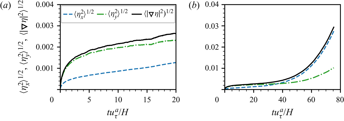
Figure 5. The temporal growth of spatial derivative statistics of surface elevation in (a) the early phase and (b) the entire wind-wave-generation stage considered. – – (blue),  $\langle \eta _x^{2}\rangle ^{1/2}$; – - – (green), $\langle \eta _y^{2}\rangle ^{1/2}$; —— (black), $\langle |\boldsymbol {\nabla }\eta |^{2}\rangle ^{1/2}$.
3.3. Air turbulence shear stress effect
Airflow provides turbulence pressure stress and shear stress on the air–water interface, which deform the water surface and generate waves. Most wind-wave-generation models consider only the pressure effect on wave growth without accounting for the contributions of shear stress. The air turbulence shear stress has two major effects on the wave dynamics. First, air shear stress can contribute additional momentum flux to the waves through coherent structures between waves and shear stress (see Peirson & Garcia Reference Peirson and Garcia2008). As discussed in Peirson & Garcia (Reference Peirson and Garcia2008), including the wave coherent tangential stress to the wind input term could reduce the discrepancy between experiments and the exponential growth models within the Miles framework. Perrard et al. (Reference Perrard, Lozano-Durán, Rabaud, Benzaquen and Moisy2019) found that in the viscous wrinkles regime below the onset of wind-wave generation, the main contribution to the surface elevation dynamics comes from air pressure fluctuations, while the effect of air shear stress is negligibly small. Second, air shear stress drives the mean water flow and generates a sheared current at the air–water interface. The current motion modifies the dispersion relation of water waves owing to the Doppler effect. The change in the dispersion relation could affect the resonance interactions between turbulent airflow and surface waves. In this section, we numerically investigate the effects of air shear stress on the wave growth behaviours in the principal stage of wave development. We compare the evolution of surface elevation variance under the actions of air turbulent pressure fluctuations only and under both air turbulent pressure fluctuations and shear fluctuations. We also analyse the evolution of air shear stress-induced current and evaluate its effect on the dispersion of surface waves, which is found to be insignificant (§ 3.3).
Here, we present in figure 6 a comparison of surface statistics between the superresolution simulation cases (P1S1_gc and P1S0_gc) for gravity–capillary waves to examine the effects of shear stress. The notations ‘P1S1’ and ‘P1S0’ denote that the transfer of air shear stress to the water domain is turned on and off, respectively. Owing to the high water–air density ratio, in the simulation, the air sees the air–water interface as a moving deformable boundary, and the water is driven by the shear stress and normal stress at the air–water interface (Liu et al. Reference Liu, Kermani, Shen and Yue2009). In the present coupled air–water DNS solver, the air domain provides the stress information at the air–water interface to the water domain, and the water domain transfers the interface geometry and velocity information to the air domain (Yang & Shen Reference Yang and Shen2011b). The transfer of air shear stress at the air–water interface from the air domain to the water domain can be artificially turned off when we conduct simulations of wave evolution subject to air pressure fluctuations only.
Figure 6. Comparison of surface-variable statistics between case P1S1_gc and case P1S0_gc: (a) surface elevation variance; (b) pressure variance at the air–water interface; (c) mean surface velocity; (d) surface velocity fluctuations. In (c), the black dashed line shows the theoretical evolution of the mean surface velocity when a constant shear stress is applied at the water surface. In (d), both  $x$- and $y$-axes are plotted in the logarithmic scale, and the back dashed lines indicate linear growth.
Figure 6(a) shows the growth of surface elevation variance  $\langle \eta ^{2}\rangle$, which indicates that the shear effect on the wave growth is insignificant. The pressure variance at the air–water interface $\langle p^{2} \rangle$, plotted in figure 6(b), is the main source of wave generation. Meanwhile, air shear stress exerted on the air–water interface can generate currents due to the viscosity of water. Figure 6(c) shows the temporal evolution of the mean water velocity at the free surface $\langle u_s\rangle$. The subscript ‘ $s$’ denotes variables at the water surface. In the early development of wind waves, surface deformations are not significant enough to distort air turbulence structures, and thus air shear stress remains in a statistically steady state. The growth of surface current velocity can be modelled by a constant shear stress applied on the surface of an initially still deep water. In the Navier–Stokes equations in the water domain, the unsteady term and vertical viscous diffusion term are the two major terms. The convection term, pressure gradient and horizontal viscous diffusion terms can be neglected (Melville, Shear & Veron Reference Melville, Shear and Veron1998). Therefore, the governing equation for water motion can be simplified as the following diffusion equation:
 \begin{equation} \frac{\partial u^{w}}{\partial t}=\nu^{w}\frac{\partial^{2} u^{w}}{\partial z^{2}}. \end{equation}
A constant shear stress  $\tau _s$ is applied on the free surface. Therefore, the surface current velocity $u_s$ can be solved analytically (see Veron & Melville Reference Veron and Melville2001):
 \begin{equation} u_s(t)=\frac{2\tau_s}{\rho^{w}\sqrt{{\rm \pi}\nu^{w}}}\sqrt{t}.\end{equation}
Figure 6(c) shows that the mean water surface velocity  $\langle u_s\rangle$ grows with the square root of time, and (3.2) agrees well with our DNS result of the superresolution simulation of gravity–capillary waves (case P1S1_gc). Second-order statistics of surface velocity variables are shown in figure 6(d). Variables $u_s^{\prime }$ and $v^{\prime }_s$ are velocity fluctuations computed by $u_s^{\prime }=u_s-\langle u_s\rangle$ and $v_s^{\prime }=v_s-\langle v_s\rangle$, respectively. As shown, $\langle u^{\prime 2}_s\rangle$ and $\langle v^{\prime 2}_s\rangle$ grow linearly with time, which can be made analogous to a diffusion process. The intensities of velocity fluctuations decrease when the transfer of air shear stress to the water is turned off. In the present simulations, the maximum current velocity is less than $0.4 u_\tau ^{a}$ and much smaller than the phase velocity of surface waves. Therefore, the Doppler effect on the dispersion relation of surface waves can be neglected.
4. Theory of wave dynamics in the principal stage
In this section, we first revisit the Phillips (Reference Phillips1957) theory on the principal stage of wind-wave generation in § 4.1. In §§ 4.2 and 4.3, a random sweeping model for turbulence air pressure fluctuations is then introduced to obtain a closure model for wave development in the principal stage of the Phillips theory. In § 4.3, the asymptotic solution of the expected value of the wave energy spectrum is calculated.
4.1. Wave evolution in the spectral space
We first revisit Phillips’ theory of the principal stage of wind-wave generation (Phillips Reference Phillips1957). Assuming that the water is inviscid and irrotational, the evolution of surface waves is governed by the following equations of the surface elevation  $\eta (\boldsymbol x,t)$ and surface velocity potential $\psi (\boldsymbol x,t)$ subject to the external forcing from the air pressure fluctuations $p(\boldsymbol x,t)$ (see Zakharov Reference Zakharov1968; Lannes Reference Lannes2013):
 $$\begin{gather} \frac{\partial \eta}{\partial t}-G[\eta]\psi=0, \end{gather}$$
 $$\begin{gather}\frac{\partial \psi}{\partial t}+g\eta - \frac{\sigma}{\rho^{w}}\boldsymbol{\nabla}\boldsymbol{\cdot}\frac{\boldsymbol{\nabla}\eta}{\sqrt{1+\left|\boldsymbol{\nabla}\eta\right|^{2}}} +\frac{1}{2}|\boldsymbol{\nabla}\psi|^{2}-\frac{(G[\eta]\psi+\boldsymbol{\nabla}\eta\boldsymbol{\cdot}\boldsymbol{\nabla}\psi)^{2}} {2(1+|\boldsymbol{\nabla}\eta|^{2})}+\frac{p}{\rho^{w}}=0. \end{gather}$$
Here,  $\boldsymbol {\nabla }=(\partial _x, \partial _y)$ is the horizontal gradient operator, and $G[\eta ]$ is the Dirichlet-to-Neumann operator, $G[\eta ]: \psi \rightarrow \sqrt {1+|\boldsymbol {\nabla }\eta |^{2}}\partial _n\phi |_{z=\eta }$, where $\partial _n$ denotes the upward normal derivative and $\phi$ is the water velocity potential satisfying the Laplacian equation in the water domain. The surface velocity potential $\psi$ is defined as the value of velocity potential $\phi$ at the free surface, i.e. $\psi (\boldsymbol x,t)=\phi (\boldsymbol x, z, t)|_{z=\eta (\boldsymbol x,t)}$ (Zakharov Reference Zakharov1968). The Dirichlet-to-Neumann operator $G[\eta ]$ is non-local and nonlinearly dependent on the surface elevation $\eta$. Assuming that the surface elevation and wave slope are infinitesimally small and the water depth is infinity, the Dirichlet-to-Neumann operator is reduced to the operator $|\boldsymbol {\nabla }|$ in the sense of Fourier multiplier by linearisation around $\eta =0$. Therefore, by eliminating surface velocity potential $\psi$ in (4.1) and (4.2), we obtain a single evolution equation for surface elevation $\eta$ to describe the dynamics of linear waves subject to external air pressure forcing
 \begin{equation} \frac{\partial^{2}\eta}{\partial t^{2}}+\left(g-\frac{\sigma}{\rho^{w}}\varDelta\right)|\boldsymbol{\nabla}|\eta={-}\frac{|\boldsymbol{\nabla}|}{\rho^{w}}p(\boldsymbol x,t).\end{equation}
Here,  $\varDelta$ is the Laplacian operator. Equation (4.3) is a linear and non-local evolution equation for $\eta$, which shows a dispersive feature of surface waves: waves of different wavelength propagate at different phase speeds.
For deep water waves, nonlinear four-wave interactions play an important role in energy exchange among different wave modes (see, e.g. Phillips Reference Phillips1960; Hasselmann Reference Hasselmann1962, Reference Hasselmann1963; Zakharov Reference Zakharov1968). Equation (4.3) is linear with respect to  $\eta$, and this linearity indicates that there exist no interactions between different wave modes. As discussed in Hammack & Henderson (Reference Hammack and Henderson1993) and Hammack & Henderson (Reference Hammack and Henderson1993), the time scale for nonlinear four-wave interactions is $O(\epsilon ^{-4}\varLambda ^{-1})$, where $\epsilon$ and $\varLambda$ are the typical wave slope and angular frequency, respectively. This scaling indicates that the nonlinear wave–wave interaction becomes significant when the wave slope is large or the wavenumber is high. As shown in figure 5(a), the wave slope $\epsilon$ in the principal stage is less than $3\times 10^{-3}$. For gravity–capillary waves with wavenumbers in the range $kl_c\leq 3.36$, the time scale of $\varLambda ^{-1}$ is larger than $4\times 10^{-3}H/u_\tau ^{a}$. Therefore, the time scale for nonlinear four-wave interactions $O(\epsilon ^{-4}\varLambda ^{-1})$ is $O(10^{6})$ larger than the duration of principal stage, i.e. $20H/u_\tau ^{a}$. The above analysis shows that the nonlinear wave–wave interactions are insignificant in the principal stage of wave development and the linear wave theory (see (4.3)) is adequate to describe the wave dynamics.
At time  $t=0$, the water is still, and the surface is flat, i.e. $\eta |_{t=0}=\partial _t\eta |_{t=0}=0$. The air pressure fluctuations are assumed to be statistically steady, and its space–time Fourier transform decays at high frequencies.
The Fourier transform  $\mathcal {F}$ and its inverse $\mathcal {F}^{-1}$ for single-variable functions are defined as
 $$\begin{gather} \mathcal{F}\{f(x)\}(k)=\frac{1}{2{\rm \pi}}\int_{-\infty}^{\infty} \, {\rm e}^{-\mathrm{i} kx}f(x)\,{\rm d}\kern0.06em x, \end{gather}$$
 $$\begin{gather}\mathcal{F}^{{-}1}\{g(k)\}(x)=\int_{-\infty}^{\infty} \, {\rm e}^{\mathrm{i}kx}g(k)\, {{\rm d}}k. \end{gather}$$
The above Fourier transform and its inverse can be extended to multivariable functions, and for variable  $f(\boldsymbol x,t)$ with two dimensions in space and one dimension in time, we use $\hat f(\boldsymbol k,t )$ to denote its spatial Fourier transform and $\tilde {f}(\boldsymbol k, \omega )$ to denote its space–time Fourier transform, i.e.
 $$\begin{gather} \hat{f}(\boldsymbol k, t)=\frac{1}{(2{\rm \pi})^{2}}\int_{\boldsymbol x\in \mathbb{R}^{2}} \, {\rm e}^{-\mathrm{i}\boldsymbol k\boldsymbol{\cdot} \boldsymbol x}f(\boldsymbol x,t)\, \mathrm{d}\boldsymbol x, \end{gather}$$
 $$\begin{gather}\tilde{f}(\boldsymbol k, \omega)=\frac{1}{(2{\rm \pi})^{3}}\int_{t\in \mathbb{R}}\int_{\boldsymbol x\in \mathbb{R}^{2}} \, {\rm e}^{-\mathrm{i}(\boldsymbol k\boldsymbol{\cdot} \boldsymbol x-\omega t)}f(\boldsymbol x,t)\, \mathrm{d}\boldsymbol x\, \mathrm{d} t, \end{gather}$$
where  $\mathbb {R}$ and $\mathbb {R}^{2}$ denote the real space with dimension one and dimension two, respectively.
Taking the spatial Fourier transform in  $\boldsymbol x$ for (4.3), we obtain
 \begin{equation} \frac{\partial^{2}}{\partial t^{2}}\hat\eta(\boldsymbol k,t)+\varLambda^{2}(\boldsymbol k)\hat\eta(\boldsymbol k)={-}\frac{k}{\rho^{w}}\hat p(\boldsymbol k,t),\end{equation}
where  $\hat \eta$ and $\hat p$ denote the spatial Fourier transform of surface elevation $\eta$ and surface pressure $p$, respectively, and $\varLambda =\sqrt {g|\boldsymbol k|+\sigma (\rho ^{w})^{-1}|\boldsymbol k|^{3}}$ is the dispersion relation of gravity–capillary waves. The surface tension $\sigma$ equals zero for gravity waves. Equation (4.8) describes the evolution of linear surface waves with small wave steepness in an inviscid deep water. Perrard et al. (Reference Perrard, Lozano-Durán, Rabaud, Benzaquen and Moisy2019) considered the viscous effect of a liquid and presented a rigorous derivation of the wrinkle dynamics in a statistically steady state where viscous dissipation balances turbulent air input. In the present study, we focus on the unsteady process of early-stage wind-wave generation. The viscous effect on the wave dynamics can be neglected owing to the low viscosity of water.
The solution of  $\hat \eta (\boldsymbol k,t)$ subject to the homogeneous initial boundary condition $\hat \eta (\boldsymbol k,t)|_{t=0}=0$ and $\partial _t \hat \eta (\boldsymbol k,t)|_{t=0}=0$ can be explicitly integrated as
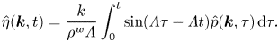 \begin{equation} \hat\eta(\boldsymbol k,t)=\frac{k}{\rho^{w}\varLambda}\int_0^{t}\sin(\varLambda \tau-\varLambda t)\hat p(\boldsymbol k,\tau)\, {{\rm d}} \tau. \end{equation}
Therefore, the wave energy component in Fourier space has the following expression:
 \begin{align} \hat\eta^{*}(\boldsymbol k,t)\hat\eta(\boldsymbol k,t)&=\frac{k^{2}}{2\rho^{w2}\varLambda^{2}}\int_0^{t} \int_0^{t} (\cos(\varLambda(\tau_2-\tau_1))-\cos (\varLambda(\tau_1+\tau_2-2t))) \nonumber\\ &\quad \hat p^{*}(\boldsymbol k, \tau_1) \hat p(\boldsymbol k,\tau_2)\, {{\rm d}} \tau_1 \, {{\rm d}} \tau_2, \end{align}
where the superscript ‘ $*$’ denotes the complex conjugate. Equation (4.10) directly indicates a key property of wind-generated waves: the wave energy component at a certain time $t$ is correlated with the entire evolution of pressure fluctuations in the previous duration $[0,t]$.
The spectrum function of pressure fluctuations naturally arises when we evaluate (4.10) in an ensemble sense. The expected value for the pressure term  $\hat p(\boldsymbol k, \tau _1) \hat p^{*}(\boldsymbol k,\tau _2)$ only depends on the wavenumber $\boldsymbol k$ and the time separation $\tau _1-\tau _2$, and we have the following relation:
 \begin{equation} \mathbb{E}[\hat p^{*}(\boldsymbol k, \tau_1) \hat p(\boldsymbol k,\tau_2)]=\hat\varPi_p(\boldsymbol k,\tau_2-\tau_1). \end{equation}
Here,  $\mathbb {E}[\cdot ]$ denotes the expected value of a statistical variable, and $\hat \varPi _p(\boldsymbol k, \boldsymbol t)$ is the spatial Fourier transform of the two-point, two-time autocovariance of pressure fluctuations $\varPi _p(\boldsymbol x, \boldsymbol t)$,
 \begin{equation} \varPi_p(\boldsymbol x, \boldsymbol t)=\langle p(\boldsymbol x+\boldsymbol x^{\prime}, t+t^{\prime}) p(\boldsymbol x^{\prime}, t^{\prime}) \rangle_{\boldsymbol x^{\prime}, t^{\prime}}, \end{equation}
where the averaging is conducted in both space and time. The two-point, one-time autocorrelation of surface elevations  $\varPsi _{\eta }(\boldsymbol x,t)$ is defined as
 \begin{equation} \varPsi_{\eta}(\boldsymbol x,t)=\langle\eta(\boldsymbol x+\boldsymbol x^{\prime},t)\eta(\boldsymbol x^{\prime},t)\rangle_{\boldsymbol x^{\prime}}, \end{equation}
where the averaging is conducted in space, and its spatial Fourier transform  $\hat \varPsi _{\eta }(\boldsymbol k,t)$ is the wave energy component $\hat \eta ^{*}(\boldsymbol k,t)\hat \eta (\boldsymbol k,t)$, i.e. (see Phillips Reference Phillips1957)
 \begin{equation} \hat\varPsi_{\eta}(\boldsymbol k,t)=\hat\eta^{*}(\boldsymbol k,t)\hat\eta(\boldsymbol k,t).\end{equation}
The expected value of the wave energy component  $\hat \varPsi _{\eta }(\boldsymbol k, t)$ is related to the wavenumber–frequency spectrum of the pressure autocovariance $\tilde {\varPi }_p(\boldsymbol k,\omega )$ and the dispersion relation of water waves $\varLambda (\boldsymbol k)$. Taking the expected values on both sides of (4.10), we obtain
 \begin{align} \mathbb{E}[\hat\varPsi_{\eta}](\boldsymbol k,t)&=\frac{k^{2}}{2\rho^{w2}\varLambda^{2}}\int_0^{t} \int_0^{t} (\cos(\varLambda(\tau_2-\tau_1))\nonumber\\ &\quad -\cos(\varLambda(\tau_1+\tau_2-2t)))\hat{\varPi}_p(\boldsymbol k,\tau_1-\tau_2)\, {{\rm d}} \tau_1 \, {{\rm d}} \tau_2. \end{align}
Phillips (Reference Phillips1957) obtained the long-term asymptotic solution of the expected value of the wave energy spectrum in each wave mode  $\boldsymbol k$,
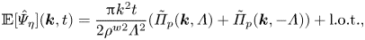 \begin{equation} \mathbb{E}[\hat\varPsi_{\eta}](\boldsymbol k,t)=\frac{{\rm \pi} k^{2}t}{2\rho^{w2} \varLambda^{2}}(\tilde{\varPi}_p(\boldsymbol k,\varLambda)+ \tilde{\varPi}_p(\boldsymbol k,-\varLambda))+\mathrm{l.o.t.},\end{equation}
where  $\mathrm {l.o.t.}$ denotes lower-order terms. The expected value of surface elevation variance in the physical space is obtained via the inverse Fourier transform,
 \begin{equation} \mathbb{E}[\langle\eta^{2}\rangle](t)=\int \mathbb{E}[\hat\varPsi_{\eta}](\boldsymbol k,t) \, {{\rm d}} \boldsymbol k.\end{equation}
As shown in (4.16), the evolution of a wavefield is closely connected to the dispersion curve  $\omega = \varLambda (\boldsymbol k)$ in the wavenumber–frequency spectrum of pressure fluctuations $\tilde {\varPi }_p(\boldsymbol k,\omega )$. Modelling the term $\tilde {\varPi }_p(\boldsymbol k,\omega = \varLambda (\boldsymbol k))$ is the key to the prediction of surface elevation variance. Phillips (Reference Phillips1957) conjectured that $\tilde {\varPi }_p(\boldsymbol k,\varLambda (\boldsymbol k))$ is proportional to the inverse of wavenumber and the convection velocity of pressure fluctuations on the air–water interface, i.e. $(kU_{p})^{-1}$, and obtained an estimation of the temporal growth of the surface elevation variance (1.1). This assumption has a physical meaning that the convective time scale is proportional to the length scale of pressure fluctuations $k^{-1}$ divided by the convection velocity of pressure fluctuations $U_{p}$. Nevertheless, the scaling factor could not be rigorously determined within the Phillips framework. Phillips noted this assumption as a ‘rough approximation’ in his original paper (see Phillips Reference Phillips1957, p. 437) and chose the scaling factor as $1$ approximately to close (4.16). A more quantitative model needs to be established with the space–time correlation properties of pressure fluctuations taken into consideration.
4.2. Random sweeping model for air pressure fluctuations
To quantitatively model the behaviours of the pressure-fluctuation wavenumber–frequency spectrum  $\tilde {\varPi }_p(\boldsymbol k,\omega )$ on the dispersion curve $\omega =\varLambda (\boldsymbol k)$, we need to characterise the decay of $\tilde {\varPi }_p$ in the frequency domain, i.e. along the $\omega$-axis. Taylor's frozen hypothesis (Taylor Reference Taylor1938) uses a Dirac delta function $\delta$ to model the wavenumber–frequency spectrum, i.e. $\tilde {\varPi }_p(\boldsymbol k,\omega )=\hat \varPsi _{p}(\boldsymbol k)\delta (\omega -\boldsymbol k\boldsymbol {\cdot } \boldsymbol U)$ where $\hat \varPsi _{p}$ denotes the wavenumber spectrum of pressure fluctuations, which indicates a non-physical concentration of energy on the line $\omega -\boldsymbol k\boldsymbol {\cdot } \boldsymbol U=0$ in the frequency domain, where $\boldsymbol U$ denotes the convection velocity. Inspired by the recent development of space–time correlation models for turbulent velocity fluctuations (He & Zhang Reference He and Zhang2006; Wilczek & Narita Reference Wilczek and Narita2012), we conjecture that the pressure fluctuations on the water surface are independent of each spatial Fourier mode, and each Fourier mode propagates at a convection velocity with random distortion. To capture the broadening property of the pressure wavenumber–frequency spectrum, we introduce a random sweeping model of pressure fluctuations. This method is analogous to the modelling of the wavenumber–frequency spectrum of turbulent velocity fluctuations first proposed by Wilczek & Narita (Reference Wilczek and Narita2012), which is based on the random sweeping hypothesis (Kraichnan Reference Kraichnan1964; Tennekes Reference Tennekes1975). The pressure fluctuations are convected at a velocity $\boldsymbol U+\boldsymbol v$ in time, where $\boldsymbol U$ is the mean convection velocity and $\boldsymbol v$ is a two-dimensional random sweeping velocity,
 \begin{equation} \frac{\partial}{\partial t}\hat p(\boldsymbol k,t)={-}\mathrm{i}\boldsymbol k \boldsymbol{\cdot} (\boldsymbol U+\boldsymbol v)\hat p(\boldsymbol k,t).\end{equation}
The random sweeping velocity  $\boldsymbol v$ satisfies the multivariate Gaussian distribution of a zero mean and a variance $\boldsymbol \varSigma$. Here, $\boldsymbol \varSigma$ is a two-by-two positive definite matrix. Equation (4.18) yields the evolution of pressure fluctuation in the spectral space,
 \begin{equation} \hat{p}(\boldsymbol k,t)=\hat{p}(\boldsymbol k,0)\exp(-\mathrm{i}\boldsymbol k \boldsymbol{\cdot} (\boldsymbol U+\boldsymbol v)t). \end{equation}
Therefore, the two-time energy spectrum of pressure fluctuations  $\hat \varPi _{p}(\boldsymbol k,\tau )$ is computed by
 \begin{align} \hat\varPi_p(\boldsymbol
k,\tau)&=\mathbb{E}[\langle\hat p^{*}(\boldsymbol k,t) \hat
p(\boldsymbol k,t+\tau)\rangle]=\hat\varPi_p(\boldsymbol
k,0)\exp(-\mathrm{i}\boldsymbol k \boldsymbol{\cdot}
\boldsymbol U\tau)\mathbb{E}[\exp(-{\rm i}\boldsymbol
k\boldsymbol{\cdot}\boldsymbol v\tau)] \nonumber\\
&=\hat\varPi_p(\boldsymbol k,0)\exp(-\mathrm{i}\boldsymbol
k \boldsymbol{\cdot} \boldsymbol U\tau)\exp
\left(-\frac{1}{2}\boldsymbol
k\boldsymbol\varSigma\boldsymbol k^{\mathsf{\text{T}}}
\tau^{2}\right), \end{align}
\begin{align} \hat\varPi_p(\boldsymbol
k,\tau)&=\mathbb{E}[\langle\hat p^{*}(\boldsymbol k,t) \hat
p(\boldsymbol k,t+\tau)\rangle]=\hat\varPi_p(\boldsymbol
k,0)\exp(-\mathrm{i}\boldsymbol k \boldsymbol{\cdot}
\boldsymbol U\tau)\mathbb{E}[\exp(-{\rm i}\boldsymbol
k\boldsymbol{\cdot}\boldsymbol v\tau)] \nonumber\\
&=\hat\varPi_p(\boldsymbol k,0)\exp(-\mathrm{i}\boldsymbol
k \boldsymbol{\cdot} \boldsymbol U\tau)\exp
\left(-\frac{1}{2}\boldsymbol
k\boldsymbol\varSigma\boldsymbol k^{\mathsf{\text{T}}}
\tau^{2}\right), \end{align}
where  $\boldsymbol k^{\mathsf{\text{T}}}$ is the transpose of the one-by-two wavenumber vector $\boldsymbol k=(k_x,k_y)$. We note that the two-time energy spectrum is related to the expected value of the energy spectrum by $\hat {\varPi }_{p}(\boldsymbol k, 0)=\mathbb {E}[\hat {\varPsi }_{p}](\boldsymbol k)$. The wavenumber–frequency spectrum of pressure fluctuations can be derived via Fourier transform,
 \begin{equation} \tilde{\varPi}_p(\boldsymbol k,\omega)=\frac{\hat\varPi_p(\boldsymbol k,0)}{\sqrt{2{\rm \pi} \boldsymbol k\boldsymbol\varSigma\boldsymbol k^{\mathsf{\text{T}}}}}\exp\left(-\frac{(\omega - \boldsymbol k \boldsymbol{\cdot} \boldsymbol U)^{2}}{2 \boldsymbol k\boldsymbol\varSigma\boldsymbol k{\mathsf{\text{T}}}}\right).\end{equation}
The positive–definite quadratic form  $\boldsymbol k\boldsymbol \varSigma \boldsymbol k^{\mathsf{\text{T}}}$ represents the strength of the random sweeping velocity of pressure fluctuations and can be determined through the following integral identity:
 \begin{equation} \int_{-\infty}^{\infty}\left(\frac{1}{\sqrt{2{\rm \pi} \boldsymbol k\boldsymbol\varSigma\boldsymbol k^{\mathsf{\text{T}}}}}\exp\left(-\frac{(\boldsymbol k \boldsymbol{\cdot} \boldsymbol U -\omega)^{2}}{2\boldsymbol k\boldsymbol\varSigma\boldsymbol k^{\mathsf{\text{T}}}}\right)\right)^{2}\, {{\rm d}} \omega=\frac{1}{2\sqrt{{\rm \pi}\boldsymbol k\boldsymbol\varSigma\boldsymbol k^{\mathsf{\text{T}}}}}. \end{equation}
Therefore,  $\sqrt {\boldsymbol k\boldsymbol \varSigma \boldsymbol k^{\mathsf{\text{T}}}}$ can be determined by
 \begin{equation} \sqrt{\boldsymbol k\boldsymbol\varSigma\boldsymbol k^{\mathsf{\text{T}}}} =\frac{\displaystyle \left(\int_{-\infty}^{\infty}\tilde{\varPi}_p(\boldsymbol k, \omega) \, {{\rm d}} \omega\right)^{2}}{\displaystyle 2\sqrt{\rm \pi}\int_{-\infty}^{\infty} \tilde{\varPi}_p^{2}(\boldsymbol k, \omega)\, {{\rm d}} \omega}. \end{equation}
The square root of the quadratic form,  $\sqrt {\boldsymbol k\boldsymbol \varSigma \boldsymbol k^{\mathsf{\text{T}}}}$, represents the angular velocity of random sweeping events, which is analogous to the angular convection velocity $\boldsymbol k \boldsymbol {\cdot } \boldsymbol U$. From (4.21), we can obtain the expression of $\boldsymbol k \boldsymbol {\cdot } \boldsymbol U$ in the wavenumber space (Del Álamo & Jiménez Reference Del Álamo and Jiménez2009),
 \begin{equation} \boldsymbol k \boldsymbol{\cdot} \boldsymbol U=\frac{\displaystyle \int_{-\infty}^{\infty} \tilde{\varPi}_p(\boldsymbol k, \omega)\omega\, \mathrm{d}\omega}{\displaystyle \int_{-\infty}^{\infty} \tilde{\varPi}_p(\boldsymbol k, \omega)\, \mathrm{d}\omega}. \end{equation}
 We plot contours of  $\boldsymbol k \boldsymbol {\cdot } \boldsymbol U$ and $\sqrt {\boldsymbol k\boldsymbol \varSigma \boldsymbol k^{\mathsf{\text{T}}}}$ in the wavenumber space $(k_x,k_y)$ to understand the distributions of these angular velocities. As shown in figure 7, both the variations of $\boldsymbol k \boldsymbol {\cdot } \boldsymbol U$ and $\sqrt {\boldsymbol k\boldsymbol \varSigma \boldsymbol k^{\mathsf{\text{T}}}}$ are much larger in the $k_x$-direction than in the $k_y$-direction. The $k_y$-related terms can be treated as higher-order perturbations relative to the $k_x$-related terms, i.e.
 $$\begin{gather} \boldsymbol k \boldsymbol{\cdot} \boldsymbol U=k_xU_{p}+\mathrm{h.o.t.}, \end{gather}$$
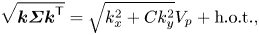 $$\begin{gather}\sqrt{\boldsymbol k\boldsymbol \varSigma\boldsymbol k^{\mathsf{\text{T}}}}=\sqrt{k_x^{2}+Ck_y^{2}}V_{p}+\mathrm{h.o.t.}, \end{gather}$$
where  $\mathrm {h.o.t}$ denotes higher-order terms. Equation (4.26) shows that the quadratic form ${\boldsymbol k\boldsymbol \varSigma \boldsymbol k^{\mathsf{\text{T}}}}$ has a diagonal leading-order approximation where $C<1$ is a constant. Wilczek, Stevens & Meneveau (Reference Wilczek, Stevens and Meneveau2015) suggest $C=0.41$ for modelling the wavenumber–frequency turbulence velocity spectrum in the logarithmic layer. We adopt $C=0.41$ for the reconstruction of pressure fluctuation spectrum in the present study. The effect of the value of $C$ on the wave spectrum and wave-growth rate in the principal stage is further discussed in § 3 of the supplementary materials. Thus, the leading-order approximations of vector $\boldsymbol U$ and matrix $\boldsymbol \varSigma$ can be written as
 $$\begin{gather} \boldsymbol U=(U_{p},0)+\mathrm{h.o.t.}, \end{gather}$$
 $$\begin{gather}\boldsymbol\varSigma=\begin{bmatrix} V_{p}^{2} & 0\\0 & CV_{p}^{2} \end{bmatrix}+\mathrm{h.o.t.}, \end{gather}$$
where the scalar quantities  $U_{p}$ and $V_{p}$ are defined as the magnitudes of the streamwise convection velocity and streamwise sweeping velocity of pressure fluctuations, respectively, both of which are only dependent on the wavenumber $k_x$. We can formally define the sweeping velocity vector $\boldsymbol V=(V_{p},\sqrt {C}V_{p})$ such that $\sqrt {\boldsymbol k\boldsymbol \varSigma \boldsymbol k^{\mathsf{\text{T}}}}=|\boldsymbol k \boldsymbol {\cdot } \boldsymbol V|+\mathrm {h.o.t.}$ to simplify notations in further derivations. The convection velocity and sweeping velocity can be numerically calculated from the wavenumber–frequency spectrum of pressure fluctuations by
 $$\begin{gather} U_{p}(k_x)=\frac{\displaystyle \int_{-\infty}^{\infty}\int_{-\infty}^{\infty} \tilde{\varPi}_p(k_x,k_y,\omega)\omega\, \mathrm{d}k_y\, \mathrm{d}\omega}{\displaystyle k_x\int_{-\infty}^{\infty} \int_{-\infty}^{\infty}\tilde{\varPi}_p(k_x,k_y,\omega)\, \mathrm{d}k_y\, \mathrm{d}\omega}, \end{gather}$$
 $$\begin{gather}V_{p}(k_x)=\frac{\displaystyle \left(\int_{-\infty}^{\infty}\int_{-\infty}^{\infty} \tilde{\varPi}_p(k_x,k_y,\omega)\, \mathrm{d}k_y\, \mathrm{d} \omega\right)^{2}}{\displaystyle 2\sqrt{\rm \pi}k_x\int_{-\infty}^{\infty}\left(\int_{-\infty}^{\infty} \tilde{\varPi}_p(k_x,k_y,\omega)\, \mathrm{d}k_y\right)^{2}\, \mathrm{d}\omega}. \end{gather}$$
Therefore, the wavenumber–frequency spectrum of pressure fluctuations can be modelled via the convection velocity vector  $\boldsymbol U$ and the sweeping velocity vector $\boldsymbol V$,
 \begin{equation} \tilde{\varPi}_p(\boldsymbol k,\omega)=\frac{\hat\varPi_p(\boldsymbol k,0)}{\sqrt{2{\rm \pi} }|\boldsymbol k \boldsymbol{\cdot} \boldsymbol V|}\exp\left(-\frac{(\omega - \boldsymbol k \boldsymbol{\cdot} \boldsymbol U)^{2}}{2(\boldsymbol k \boldsymbol{\cdot} \boldsymbol V)^{2}}\right).\end{equation}
Figure 7. Contours of (a)  $\boldsymbol k \boldsymbol {\cdot } \boldsymbol U$ and (b) $\sqrt {\boldsymbol k\boldsymbol \varSigma \boldsymbol k^{\mathsf{\text{T}}}}$ normalised by their maximum values, respectively, in the wavenumber space. For both $\boldsymbol k \boldsymbol {\cdot } \boldsymbol U$ and $\sqrt {\boldsymbol k\boldsymbol \varSigma \boldsymbol k^{\mathsf{\text{T}}}}$, variations in the $k_x$-direction are much more significant than those in the $k_y$-direction.
Figure 8 visualises the present wavenumber–frequency model for pressure fluctuations at the air–water interface. The convection velocity  $U_{p}$ and the sweeping velocity $V_{p}$ are plotted in figures 8(a) and 8(b), respectively. The convection velocity decays as the wavenumber increases, indicating that the larger-scale pressure fluctuations move faster. This phenomenon is consistent with previous studies (see Choi & Moin Reference Choi and Moin1990; Luhar, Sharma & McKeon Reference Luhar, Sharma and McKeon2014). The sweeping velocity $V_{p}$ shares a similar tendency, and its amplitude is smaller than the convection velocity for all wavenumbers. Figures 8(c) and 8(d) compare the wavenumber–frequency spectrum of pressure fluctuations between the DNS results and the random sweeping model. The numerical results are obtained by conducting the space–time Fourier transform using $34\,488$ consecutive snapshots of the superresolution simulation of gravity–capillary waves (case P1S1_gc). As shown, the present model directly captures the energy decay along the wavenumber $k_x$ and the broadening effect along with the frequency $\omega$ and has good agreement with the numerical results.
Figure 8. Panels (a) and (b) show the convection velocity  $U_{p}(k_x)$ and sweeping velocity $V_{p}(k_x)$ of turbulent pressure at the water surface, respectively. (c) The DNS results of the wavenumber–frequency spectrum of pressure fluctuations averaged in the $y$-direction, $S=\langle \tilde {\varPi }_p\rangle _y$. (d) The random sweeping model for the wavenumber–frequency spectrum of pressure fluctuations averaged in the $y$-direction.
In the present model, we adopt a Gaussian distribution to depict the dependence of the wavenumber–frequency spectrum  $\tilde \varPi _p(\boldsymbol k,\omega )$ on the frequency variable $\omega$. We note that the Gaussian distribution assumption is not a rigorous approach for the wavenumber–frequency spectrum, and the frequency spectrum reveals a non-Gaussian shape due to the intermittency effects in turbulence (Choi & Moin Reference Choi and Moin1990; Farabee & Casarella Reference Farabee and Casarella1991; Hu et al. Reference Hu, Morfey and Sandham2006). Although theoretical frameworks of space–time characteristics of the turbulent velocity field have been established (He & Zhang Reference He and Zhang2006; Wilczek & Narita Reference Wilczek and Narita2012; Wu & He Reference Wu and He2020), modelling the wavenumber–frequency spectrum of wall pressure fluctuations is still challenging (see Luhar et al. Reference Luhar, Sharma and McKeon2014; He, Jin & Yang Reference He, Jin and Yang2017; Towne, Lozano-Durán & Yang Reference Towne, Lozano-Durán and Yang2020). The Gaussian distribution model provides the simplest approach to introduce the frequency broadening effect to linear wave theory. As shown in § 4.3 below, this approach results in reasonable predictions of wave fluctuation growth in both physical space and Fourier spectral space.
4.3. Random sweeping turbulence pressure–wave interaction model in the principal stage
We assume that the air pressure fluctuations exerted on the air–water interface satisfy the random sweeping model (4.18). The space–time evolution of pressure fluctuations can be described by the convection velocity vector  $\boldsymbol U$ and the random vector $\boldsymbol v$, of which the variance can be characterised by the sweeping velocity vector $\boldsymbol V$. We obtain a closure model governing turbulence–wave interactions, which is referred to as the random sweeping turbulence pressure–wave interaction model, and the wave evolution equation in the spatial Fourier space (4.8) becomes
 \begin{equation} \frac{\partial^{2}}{\partial t^{2}}\hat\eta(\boldsymbol k,t)+\varLambda^{2}(\boldsymbol k)\hat\eta(\boldsymbol k)={-}\frac{k}{\rho^{w}}\hat p(\boldsymbol k,0)\exp(-\mathrm{i}\boldsymbol k \boldsymbol{\cdot} (\boldsymbol U+\boldsymbol v)t).\end{equation}
For any wavenumber  $\boldsymbol k$, (4.32) can be viewed as a stochastic ordinary differential equation with respect to time $t$, and the corresponding statistical quantities can be analytically evaluated. The expected value of the wave energy spectrum has the following integral expression:
 \begin{align} \mathbb{E}[\hat\varPsi_{\eta}](\boldsymbol k,t)&=\frac{k^{2}\hat{\varPi}_p(\boldsymbol k,0)}{2\rho^{w2}\varLambda^{2}}\int_0^{t} \int_0^{t} (\cos(\varLambda(\tau_2-\tau_1))-\cos(\varLambda(\tau_1+\tau_2-2t)))\nonumber\\ &\quad \exp(-\mathrm{i}\boldsymbol k \boldsymbol{\cdot} \boldsymbol U(\tau_1-\tau_2))\exp \left(-\frac{1}{2}(\boldsymbol k \boldsymbol{\cdot} \boldsymbol V)^{2}(\tau-\tau_2)^{2}\right)\, {{\rm d}} \tau_1 \, {{\rm d}} \tau_2. \end{align}
Equation (4.33) is deterministic in time, and the double integral on its right-hand side leads to an algebraic solution, which is shown in Appendix D as (D5)–(D7). Utilising the properties of the Gaussian function in the expression (4.33), we can conduct rigorous asymptotic analysis on the expected value of the wave energy spectrum in the next section.
4.4. Asymptotic solution of  $\mathbb {E}[\hat \varPsi _{\eta }]$

In the wavenumber space, the expected value of the wave energy spectrum  $\mathbb {E}[\hat \varPsi _{\eta }](\boldsymbol k,t)$ in (4.33) can be written in the following asymptotic expansion for a large time $t$:
$t$:
 \begin{equation} \mathbb{E}[\hat\varPsi_{\eta}](\boldsymbol k,t)= \varTheta_1+ \varTheta_2+\varTheta_3+\cdots,\end{equation}
with  $\varTheta _i(i=1,2,3,\ldots )$ being the first $i$th term in the asymptotic expansion of $\mathbb {E}[\hat \varPsi _{\eta }]$ with respect to time $t$. The asymptotic solution can be calculated as
 \begin{align} \varTheta_1&= \frac{\sqrt{2{\rm \pi}}k^{2}\hat \varPi_p(\boldsymbol k,0)t}{4\rho^{w2}\varLambda^{2} |\boldsymbol k \boldsymbol{\cdot} \boldsymbol V|}\left(\exp\left(-\frac{(\boldsymbol k \boldsymbol{\cdot} \boldsymbol U - \varLambda)^{2}}{2 (\boldsymbol k \boldsymbol{\cdot} \boldsymbol V)^{2}}\right) + \exp\left(-\frac{(\boldsymbol k \boldsymbol{\cdot} \boldsymbol U + \varLambda)^{2}}{2(\boldsymbol k \boldsymbol{\cdot} \boldsymbol V)^{2}}\right)\right),\end{align}
 \begin{align} \varTheta_2&={-}\frac{\sqrt{2{\rm \pi}}k^{2}\hat{\varPi}_p(\boldsymbol k,0)\sin(2\varLambda t)}{8\rho^{w2}\varLambda^{3}|\boldsymbol k \boldsymbol{\cdot} \boldsymbol V|}\left(\exp\left(-\frac{(\boldsymbol k \boldsymbol{\cdot} \boldsymbol U+\varLambda)^{2}}{2(\boldsymbol k \boldsymbol{\cdot} \boldsymbol V)^{2}}\right)+\exp\left(-\frac{(\boldsymbol k \boldsymbol{\cdot} \boldsymbol U-\varLambda)^{2}}{2(\boldsymbol k \boldsymbol{\cdot} \boldsymbol V)^{2}}\right)\right) \nonumber\\ &\quad +\frac{\sqrt{2}k^{2}\hat{\varPi}_p(\boldsymbol k,0)\cos(2\varLambda t)}{4\rho^{w2}\varLambda^{3}|\boldsymbol k \boldsymbol{\cdot} \boldsymbol V|}\left({{D}_+}\left(\frac{\boldsymbol k \boldsymbol{\cdot} \boldsymbol U+\varLambda}{\sqrt{2}|\boldsymbol k \boldsymbol{\cdot} \boldsymbol V|}\right)-{{D}_+}\left(\frac{\boldsymbol k \boldsymbol{\cdot} \boldsymbol U-\varLambda}{\sqrt{2}|\boldsymbol k \boldsymbol{\cdot} \boldsymbol V|}\right)\right),\end{align}
 \begin{align} \varTheta_3&= \frac{\sqrt{2}k^{2}\hat{\varPi}_p(\boldsymbol k,0)}{4\rho^{w2}\varLambda^{3}|\boldsymbol k \boldsymbol{\cdot} \boldsymbol V|}\left(\frac{2\varLambda(\boldsymbol k \boldsymbol{\cdot} \boldsymbol U+\varLambda)+(\boldsymbol k \boldsymbol{\cdot} \boldsymbol V)^{2}}{(\boldsymbol k \boldsymbol{\cdot} \boldsymbol V)^{2}}{{D}_+}\left(\frac{\boldsymbol k \boldsymbol{\cdot} \boldsymbol U+\varLambda}{\sqrt{2}|\boldsymbol k \boldsymbol{\cdot} \boldsymbol V|}\right)\right. \nonumber\\ &\quad +\left.\frac{2\varLambda(\boldsymbol k \boldsymbol{\cdot} \boldsymbol U-\varLambda)-(\boldsymbol k \boldsymbol{\cdot} \boldsymbol V)^{2}}{(\boldsymbol k \boldsymbol{\cdot} \boldsymbol V)^{2}}{{D}_+}\left(\frac{\boldsymbol k \boldsymbol{\cdot} \boldsymbol U-\varLambda}{\sqrt{2}|\boldsymbol k \boldsymbol{\cdot} \boldsymbol V|}\right)-\frac{2\sqrt{2}\varLambda}{|\boldsymbol k \boldsymbol{\cdot} \boldsymbol V|}\right). \end{align}
Here,  $\varTheta _1$ is the leading-order term, which grows linearly with time, $\varTheta _2$ oscillates with time $t$, and $\varTheta _3$ is a constant independent of time $t$. The Dawson function, ${{D}_+}(x)$, is defined as
 \begin{equation} {{D}_+}(x)=e^{{-}x^{2}}\int_0^{x} \, {\rm e}^{t^{2}}\, \mathrm{d}t, \end{equation}
which is a bounded function for real  $x$. Detailed derivations can be found in Appendix D.
Next, we analyse the relative strength between  $\varTheta _1$ and $\varTheta _2$. Because $\varTheta _2$ is the summation of two trigonometric functions, we can obtain the following estimation of the ratio between $|\varTheta _2|$ and $|\varTheta _1|$ via the Cauchy–Schwartz inequality:
 \begin{equation} \frac{|\varTheta_2|}{|\varTheta_1|}\leq\frac{\varGamma }{2\varLambda t},\end{equation}
where the scaling factor  $\varGamma$ is independent of time, defined as
 \begin{equation} \varGamma =\sqrt{1+\frac{4}{\rm \pi}\left(\frac{{{D}_+}(\alpha+\beta)- {{D}_+}(\alpha-\beta)}{\exp(-(\alpha+\beta)^{2})+\exp (-(\alpha-\beta)^{2})}\right)^{2}}.\end{equation}
The two non-dimensionalised variables in (4.40) are  $\alpha =\boldsymbol k \boldsymbol {\cdot } \boldsymbol U/(\sqrt {2}|\boldsymbol k \boldsymbol {\cdot } \boldsymbol V|)$ and $\beta =\varLambda /(\sqrt {2}|\boldsymbol k \boldsymbol {\cdot } \boldsymbol V|)$.
In the expression of the leading-order asymptotic solution  $\varTheta _1$ (4.35), the Gaussian functions indicate that the growth rates of certain wavenumbers near the resonance curve $\varLambda -\boldsymbol k \boldsymbol {\cdot } \boldsymbol U=0$ are amplified. To obtain a priori estimates of the scaling factor $\varGamma$, it is sufficient to focus on the wavenumber regime near the resonance curve $\varLambda -\boldsymbol k \boldsymbol {\cdot } \boldsymbol U=0$. When the wavenumber $k$ is near the resonance curve, we have $\beta \approx \alpha$. Taking the Taylor series expansion with respect to $\beta$ around the region $\beta =\alpha$, we obtain
 \begin{equation} \varGamma =\sqrt{1+\frac{4}{\rm \pi} \left(\frac{{{D}_+}(2\alpha)}{1+\exp({-}4\alpha^{2})}\right)^{2}} +\mathcal{C}(\beta-\alpha)+\mathrm{h.o.t.},\end{equation}
where  $\mathcal {C}$ is the Taylor coefficient of the first-order expansion. By direct calculations, we can prove that $\mathcal {C}$ is a bounded function with respect to $\alpha$, which satisfies $|\mathcal {C}|< 0.5$ for all $\alpha \in \mathbb {R}$. The leading-order term in (4.41) is also a bounded function with respect to $\alpha$ and its value is close to $1$, i.e. $\varGamma \approx 1$.
In the principal stage of the Phillips theory, the time scale of wave development is larger than the development time of turbulent pressure fluctuations (Phillips Reference Phillips1957, p. 426). In the present random sweeping turbulence–wave interaction model, the tendency of the amplitude ratio between the second-order asymptotic term and the first-order asymptotic term is explicitly given in (4.39), i.e.  $|\varTheta _2/\varTheta _1|\sim (2\varLambda t)^{-1}$. When the time scale reaches $t\gg \varLambda ^{-1}$, the linear growth dominates the oscillation, and the linear-growth behaviour of ${E}[\hat \varPsi _{\eta }]$ (see (4.35)) in the wavenumber space can be observed. In the present DNS study, the time scale of $\varLambda ^{-1}$ is much smaller than the principal stage time scale. Because the dispersions of gravity–capillary waves and gravity waves are different and they both are dependent on the wavenumber, we summarise some typical values of $\varLambda ^{-1}$ and compare them with the principal stage time scale. For gravity–capillary waves with small wavenumber $kl_c=0.06$ and large wavenumber $kl_c=3.36$, the inverse of wave angular frequencies normalised by the air friction velocity and domain height, i.e. $\varLambda ^{-1}u_\tau ^{a}/H$, is $0.115$ and $0.004$, respectively. For gravity waves with small wavenumber $kl_c=0.06$ and large wavenumber $kl_c=3.36$, the time scale $\varLambda ^{-1}u_\tau ^{a}/H$ is $0.116$ and $0.015$, respectively. The time scale of the principal stage is $tu_\tau ^{a}/H\in [0,20]$ in our study. For example, when the elapsed time reaches $tu_\tau ^{a}/H=1$, the value of $t$ is at least eight times larger than $\varLambda ^{-1}$. Therefore, $t\gg \varLambda ^{-1}$ is a valid assumption for the analysis of the principal stage development.
Next, we examine the leading-order approximation of  $\varTheta _3$ when the wavenumber is located near the resonance curve. From direct calculations using (4.35) and (4.37), we obtain
 \begin{equation} \frac{\varTheta_3}{\varTheta_1}=\frac{(8\alpha+\alpha^{{-}1}) {{D}_+}(2\alpha)-4}{1+\exp({-}4\alpha^{2})}\frac{1}{\sqrt{2{\rm \pi}}|\boldsymbol k \boldsymbol{\cdot} \boldsymbol V| t}+\mathrm{h.o.t.}. \end{equation}
 The series expansion of the Dawson function gives  ${{D}_+}(x)=(2x)^{-1}+\mathrm {l.o.t.}$ for large $x$ and ${{D}_+}(x)=x+\mathrm {h.o.t.}$ for $x$ near zero. This indicates that the ratio between $\varTheta _3$ and $\varTheta _1$ is uniformly bounded for all $\alpha$.
A comparison of the temporal growth rates of the leading-order asymptotic terms can be conducted using a similar approach. We obtain the ratio of amplitudes between the time derivatives of the second-order asymptotic term  $|\partial _t\varTheta _2|$ and the first-order asymptotic term $|\partial _t\varTheta _1|$,
 \begin{equation} \frac{|\partial_t\varTheta_2|}{|\partial_t\varTheta_1|}\leq\varGamma .\end{equation}
 As shown in the discussion above, the scaling factor  $\varGamma$ is close to $1$. This indicates that the strength between the time derivatives of the first and second asymptotic terms are comparable. The overall growth behaviour of the expected value of the wave energy spectrum $\mathbb {E}[\hat \varPsi _{\eta }]$ is linear because the magnitude of $\varTheta _1$ dominates that of $\varTheta _2$ in the principal stage, as shown above. We also note that the coefficient $\mathcal {C}$ of the first-order Taylor expansion term in (4.41) does not degenerate. The scaling factor $\varGamma$ can be larger than $1$ when the wavenumber $k$ moves across the resonance curve $\varLambda -\boldsymbol k \boldsymbol {\cdot } \boldsymbol U=0$, which indicates the possibility of a negative instantaneous grow rate of $\mathbb {E}[\hat \varPsi _{\eta }](\boldsymbol k,t)$, as shown in (4.36). Therefore, the instantaneous growth rate of $\mathbb {E}[\hat \varPsi _{\eta }]$ fluctuates due to the comparable strength between $|\partial _t\varTheta _1|$ and $|\partial _t\varTheta _2|$ and can decrease to zero or even a negative value at certain times. The above theoretical analysis indicates the oscillating nature of the growth of the wave energy spectrum, which cannot be eliminated with ensemble averaging. Our DNS results confirm this conjecture, as shown below in § 5.1.
5. Comparison between theoretical and DNS results
In this section, we analyse the linear-growth behaviour of the wave energy spectrum and evaluate the existence of the principal stage in the wavenumber space (§ 5.1). The development of the wave energy spectrum is further studied using a time-dependent norm. A comparison among our present model, the Phillips model and the DNS results is performed in both the wavenumber space (§ 5.2) and the physical space (§ 5.3).
5.1. Numerical evidence of the principal stage
In this section, we compare the wave-growth behaviour in the wavenumber space between the DNS results and Phillips theory to evaluate the linear-growth conjecture of the wave energy spectrum. In the Phillips theory, the expected values of wave energy components  $\mathbb {E}[\hat {\varPsi }_{\eta }](\boldsymbol k,t)$ grow linearly with time for all wavenumbers in the principal stage. To evaluate the similarity between the evolution of $\mathbb {E}[\hat {\varPsi }_{\eta }](\boldsymbol k,t)$ and a linear function of time, we compute the similarity score $\mathcal {S}(\boldsymbol k)$, which is defined as the correlation between $\mathbb {E}[\hat {\varPsi }_{\eta }](\boldsymbol k,t)$ and the linear function $f(t)=t$
 \begin{equation} \mathcal{S} (\boldsymbol k)=\frac{\int_0^{T_M}\mathbb{E}[\hat{\varPsi}_{\eta}] t \, {{\rm d}}t}{\left(\int_0^{T_M} \mathbb{E}[\hat{\varPsi}_{\eta}]^{2} \, {{\rm d}}t\right)^{1/2}\left( \int_0^{T_M} t^{2} \, {{\rm d}}t\right)^{1/2}},\end{equation}
where  $T_M$ denotes the maximum sampling time. The score $\mathcal {S}$ varies from 0 to 1 because $\mathbb {E}[\hat {\varPsi }_{\eta }](\boldsymbol k,t)$ is a non-negative function of $t$. The score $\mathcal {S}$ equals 1 if $\mathbb {E}[\hat {\varPsi }_{\eta }](\boldsymbol k,t)$ is a perfectly linear function of $t$. Figure 9(a) depicts $\mathcal {S}(\boldsymbol k)$ in the wavenumber space $(k_x,k_y)$. The maximum sampling time $T_M$ is chosen to be $T_M=20H/u_\tau ^{a}$, which is approximately the end time for the principal stage (see figure 21), and the sampling interval is $1.44\times 10^{-2} H/u_\tau ^{a}$. Ten realisations of independent gravity–capillary wave simulations are used to conduct ensemble averaging. Contours in figure 9(a) indicate that the similarity score $\mathcal {S}$ varies between $0.73$ and $0.996$, and it is very close to $1$ in the low-wavenumber regime. Figure 9(b) visualises the distribution of the similarity score $\mathcal {S}$ as a function of $|\boldsymbol k|$ and plots the azimuthal average of $\mathcal {S}$. In the low-wavenumber regime $\{(k_x,k_y) \mid kl_c<0.8\}$, $\mathcal {S}$ at most wavenumbers is above $0.97$, which indicates that $\mathbb {E}[\hat \varPsi ](\boldsymbol k)$ grows linearly with time. There exist some wavenumbers where $\mathcal {S}$ is beyond $0.99$. The temporal growth of $\mathbb {E}[\hat {\varPsi }_{\eta }](\boldsymbol k,t)$ at these wavenumbers has a nearly perfect linear dependence on the time $t$. Figure 9(c) shows the temporal growth of wave energy components with five highest similarity scores. A scaling factor $\gamma$ is manually chosen in each case to separate curves for visualisation purpose. Black dashed lines denote linear fitting results, and the coefficient of determination values all exceed $0.966$, indicating good linear growth behaviours of wave energy components at these wavenumbers. On the other hand, in the regime where the magnitude of wavenumber $|\boldsymbol k|$ is large, the similarity score is much lower. The wave energy components $\mathbb {E}[\hat {\varPsi }_{\eta }](\boldsymbol k,t)$ at these wavenumbers do not grow monotonically with time, as shown in figure 9(d).
Figure 9. (a) Contours of the similarity score  $\mathcal {S}(\boldsymbol k)$ using continuous colour map. (b) Scatter plot of the similarity score $\mathcal {S}$ as a function of absolute wavenumber $kl_c$: $\bullet$ (blue), discretised value of similarity score $\mathcal {S}$; —— (orange), smoothed function of the similarity score $\mathcal {S}$. The similarity score $\mathcal {S}$ is close to $1$ in the low-wavenumber region. (c) Time series of wave energy components $|\hat \eta |^{2}$ at the wavenumbers with five highest similarity scores. Black dashed lines denote linear fitting. (d) Time series of four-wave energy components at high wavenumbers.
We conduct a spectral analysis of the surface elevation in the principal stage, and summarise the wavenumbers  $(k_xl_c,k_yl_c)$ and expected values of wave energy percentage $\mathbb {E}[\hat \varPsi _{\eta }/\langle \eta ^{2}\rangle ]$ of the five most energetic wave components in table 3. The expected value of wave energy percentage $\mathbb {E}[\hat \varPsi _{\eta }/\langle \eta ^{2}\rangle ]$ at the wavenumber $(k_x,k_y)$ is calculated as the ensemble average of $\hat \varPsi _{\eta }/\langle \eta ^{2}\rangle$ using ten realisations in the Group I simulations. Here, $\mathbb {E}[\hat \varPsi _{\eta }/\langle \eta ^{2}\rangle ]$ represents the relative linear-growth rate among different wavenumbers in the principal stage of wave development. For both gravity–capillary waves and gravity waves, the behaviours of the top most energetic wave components have similar features in the principal stage (i.e. $tu_\tau ^{a}/H<20$). The spanwise wavenumbers $k_y$ of these wave components are relatively larger than the streamwise wavenumbers, and the summation of energy percentages of these five most energetic wave components is less than one half of the total wave energy. The wave energy is distributed over a range of wave components, rather than concentrated in a few wavenumbers. These five most energetic waves contain approximately $33\,\%$ of the total wave energy in the principal stage, similar to the value of $28\,\%$ reported in the DNS study of Lin et al. (Reference Lin, Moeng, Tsai, Sullivan and Belcher2008). In a dimensional form, the fastest growing wave mode in the principal stage is $(k_x,k_y )=(0.20,0.82)\ \mathrm {cm}^{-1}$ in our study, which is compatible with the value of $(k_x,k_y )=(0.26,1.0)\ \mathrm {cm}^{-1}$ reported by Lin et al. (Reference Lin, Moeng, Tsai, Sullivan and Belcher2008).
Table 3. Wavenumbers and expected values of wave energy percentages for the five most energetic wave components at the time instants  $tu_\tau ^{a}/H=5,10,15$ and $20$ in the principal stage for gravity–capillary waves and gravity waves. Here, $\hat \varPsi _{\eta }$ denotes the wave energy at the wavenumber $(k_x,k_y)$ defined in (4.14). The symbol ‘sum’ represents the summation of wave energy percentages of the five most energetic wave components.
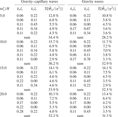
We quantitatively compare the wave-growth behaviours of the present DNS simulation in the principal stage with the previous numerical simulation by Lin et al. (Reference Lin, Moeng, Tsai, Sullivan and Belcher2008) and laboratory experiment by Zavadsky & Shemer (Reference Zavadsky and Shemer2017). Based on the air friction velocity  $u_\tau ^{a}=0.08\ \mathrm {m\ s}^{-1}$ and air domain height $H=0.0489\ \mathrm {m}$, we convert the present results to dimensional form and compare them with the literature. Figure 10(a) shows the temporal evolution of surface elevation variance of present DNS, denoted by blue line (——, blue) for Group I simulations and red line (——, red) for Group II simulations, and DNS from Lin et al. (Reference Lin, Moeng, Tsai, Sullivan and Belcher2008), denoted by marker $\square$ (black). Blue dashed lines (– –, blue) represent individual realisations of ensemble simulations in Group I. The linear-growth rates of surface elevation variance are in agreement between our results and Lin et al. (Reference Lin, Moeng, Tsai, Sullivan and Belcher2008) because the air friction velocities are close between these two DNS. We plot the linear-growth rates of our DNS results, DNS from Lin et al. (Reference Lin, Moeng, Tsai, Sullivan and Belcher2008), and the experiment of Zavadsky & Shemer (Reference Zavadsky and Shemer2017) in figure 10(b). The air friction velocities in the experimental study by Zavadsky & Shemer (Reference Zavadsky and Shemer2017) are about $6$–
$6$– $9$ times larger than our DNS. Therefore, their linear-growth rates are significantly higher than ours. The power-law scaling, $\partial _t\langle \eta ^{2}\rangle \sim (u_\tau ^{a})^{4}$, which was proposed by Zavadsky & Shemer (Reference Zavadsky and Shemer2017), is also illustrated in figure 10(b). It should be noted that the air friction velocity of DNS (i.e. $0.08\ \mathrm {m\ s}^{-1}$) is significantly beyond the parameter range of the experimental study (i.e. $0.53\ \mathrm {m\ s}^{-1}\sim 0.74\ \mathrm {m\ s}^{-1}$). Figures 11(a) and 11(b) show two examples of linear growth of $\mathbb {E}[\hat {\varPsi }_{\eta }](\boldsymbol k,t)$, where the wavenumbers are $(k_xl_c,k_yl_c)=(0.11,0)$ and $(k_xl_c,k_yl_c)=(0.45,0.34)$, respectively. The linear-growth behaviour of the expected value of the wave energy component $\mathbb {E}[\hat {\varPsi }_{\eta }](\boldsymbol k,t)$ can be clearly observed. Figures 11(c) and 11(d) are zoomed-in views of (a) and (b), respectively, during the time interval $tu_\tau ^{a}/H\in [10,11]$. Owing to the high sampling frequency, our DNS results can capture the fine oscillatory structure of the expected value of the wave energy component $\mathbb {E}[\hat {\varPsi }_{\eta }](\boldsymbol k,t)$, which is theoretically predicted in (4.43). In figures 11(c) and 11(d), the local maxima and minima are marked as red and green asterisks, respectively. We calculate the mean oscillation period $T_{os}$ for each wavenumber based on the DNS results. The dependency of $T_{os}$ on wavenumber is plotted in figure 12. In the asymptotic analysis of the expected value of the wave energy spectrum $\mathbb {E}[\hat \varPsi _{\eta }](\boldsymbol k,t)=\varTheta _1+\varTheta _2+\varTheta _3+\cdots$ (see (4.34)), the second leading-order term $\varTheta _2(\boldsymbol k,t)$ represents the temporal oscillation behaviour for the wave energy spectrum. As shown in (4.36), for any fixed wavenumber $\boldsymbol k$, the function $\varTheta _2$ evolves as a trigonometric function in time $t$;
$t$;  $\varTheta _2$ can be rewritten as $\varTheta _2=A_0\sin (2\varLambda t+\theta _0)$, where $A_0$ and $\theta _0$ are only functions of wavenumber $\boldsymbol k$. Therefore, for any wavenumber $\boldsymbol k$, $\varTheta _2(\boldsymbol k,t)$ has an angular frequency of $2\varLambda (\boldsymbol k)$ and its oscillation period $T_{os}$ is given by $T_{os}=2{\rm \pi} /(2\varLambda )={\rm \pi} /\varLambda$, where $\varLambda (\boldsymbol k)$ denotes the dispersion relation of surface waves. As shown in figures 12(a) and 12(b), the numerical periods agree well with the theoretical predictions for both gravity–capillary waves and gravity waves. The similarity between figures 12(a) and 12(b) is because the theoretical oscillation period (i.e. $T_{os}={\rm \pi} /\varLambda$) does not differ much between gravity–capillary waves and gravity waves. Owing to the dispersion relation, $T_{os}$ of gravity–capillary waves is smaller than that of gravity waves. The difference is not obvious if inspected visually because they are both monotonically decreasing functions with time. However, the capillary effects have major effects on the shape of wave energy spectrum in the wavenumber space, which is discussed in § 5.2.
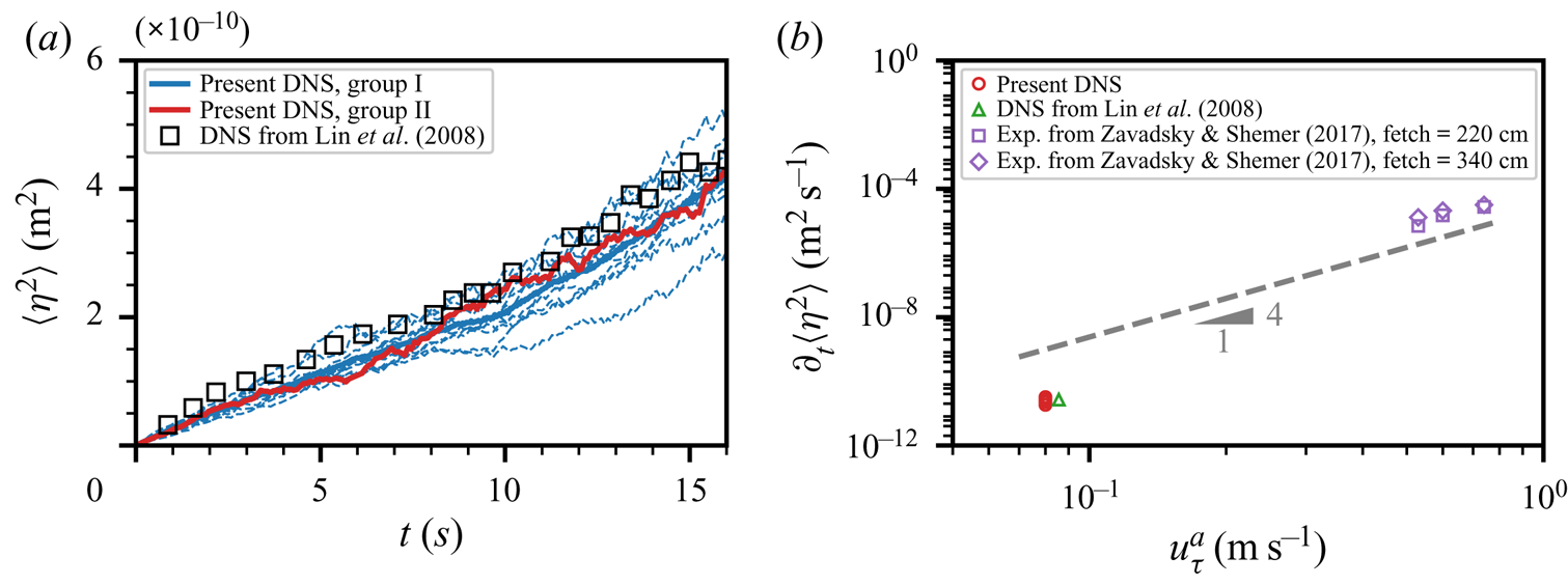
Figure 10. (a) Surface elevation variance as a function of time in the principal stage. DNS from Lin et al. (Reference Lin, Moeng, Tsai, Sullivan and Belcher2008) is denoted by  $\square$ (black). Present simulations results are denoted by: – – (blue), each realisation of ensemble simulations (Group I); —— (blue), ensemble average of Group I; —— (red), super-resolution simulation (Group II). (b) Wave linear-growth rate $\partial _t\langle \eta ^{2}\rangle$ in the principal stage as a function of air friction velocity $u_\tau ^{a}$. Numerical and measurement data are plotted for comparison: $\triangle$ (green), DNS from Lin et al. (Reference Lin, Moeng, Tsai, Sullivan and Belcher2008); $\square$ (purple) and $\Diamond$ (purple), laboratory experiments (EXP.) from Zavadsky & Shemer (Reference Zavadsky and Shemer2017) with fetch distances of $220\ \mathrm {cm}$ and $340\ \mathrm {cm}$, respectively. Present DNS results are denoted by $\circ$ (red). The dashed line (– –, grey) denotes the power-law scaling, $\partial _t\langle \eta ^{2}\rangle \sim (u_\tau ^{a})^{4}$, proposed by Zavadsky & Shemer (Reference Zavadsky and Shemer2017).
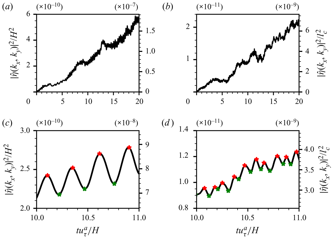
Figure 11. Temporal growth of the wave energy component  $\mathbb {E}[\hat {\varPsi }_{\eta }](\boldsymbol k,t)$ at selected wavenumbers. (a): $(k_xl_c,k_yl_c)=(0.11,0)$, and (b): $(k_xl_c,k_yl_c)=(0.45,0.34)$. Panels (c) and (d) are zoomed-in views of (a) and (b), respectively. Local maxima and minima are marked using red and green asterisks, respectively.

Figure 12. Oscillation period  $T_{os}$ of the temporal evolution of the expected value of wave energy component $\mathbb {E}[\hat \varPsi ](\boldsymbol k,t)$ for (a) gravity–capillary waves and (b) gravity waves.
The wave energy spectrum is related to the surface elevation variance via (4.17). The oscillation phenomenon of the wave energy spectrum  $\mathbb {E}[\hat \varPsi _{\eta }](\boldsymbol k,t)$, which occurs at all wavenumbers in the wavenumber space (see (4.36)), also contributes to the oscillation of the expected value of surface elevation variance $\mathbb {E}[\langle \eta ^{2}\rangle ](t)$ in the physical space. To evaluate the temporal oscillation of $\mathbb {E}[\langle \eta ^{2}\rangle ](t)$, we compute the time derivatives of instantaneous surface elevation variance $\partial _t\langle \eta ^{2}\rangle (t)$ and perform ensemble averaging on different numbers of realisations $N$. The distributions of $\partial _t\langle \eta ^{2}\rangle$ are depicted in figure 13 using Gaussian kernel density estimation. As $N$ increases, the kernel density function becomes narrower and more concentrated near the mean, of which the trend is consistent with general statistical analysis. From the asymptotic analysis on the expected value of the wave energy spectrum $\mathbb {E}[\hat {\varPsi }_{\eta }](\boldsymbol k,t)$ in § 4.4, the normalised instantaneous wave-growth rate can vary from $1-\varGamma$ to ${1+\varGamma }$ near the resonance curve where the wave-growth rates are mostly amplified with the scaling factor $\varGamma \approx 1$. This result indicates that the expected values of the normalised instantaneous wave-growth rates have a finite variance, and the temporal oscillation of $\mathbb {E}[\langle \eta ^{2}\rangle ](t)$ cannot be eliminated when the number of realisations $N$ approaches infinity. The margins of theoretically predicted oscillation interval $[1-\varGamma,1+\varGamma ]$ are marked using the vertical dashed lines in figure 13(a). We further calculate the interval $(1-1.96\sigma,1+1.96\sigma )$ which includes $95\,\%$ of the normalised $\partial _t\langle \eta ^{2}\rangle$ in the Gaussian distribution assumption. Here, $\sigma$ denotes the normalised variance. In figure 13(b), we plot the interval width, defined as $L_{95}=3.92\sigma /\mu$, among different numbers of realisations together with the idealised width of estimation, $2\varGamma$. We note that while the trend is clear, it is desirable to have a larger number of realisations $N$ to further confirm the above analysis. However, as described in § 2.3, the DNS is computationally expensive. With the currently available computing power, we can only afford ten realisations.

Figure 13. (a) Kernel density estimations of instantaneous growth rate  $\partial _t\langle \eta ^{2}\rangle$, normalised by the time-averaged mean. Legends indicate the number of realisations $N$. Two vertical dashed lines depict the theoretically predicted upper and lower bounds. (b) The width of the interval containing $95\,\%$ of total data, $L_{95}$, among different $N$. The blue dashed line indicates the idealised width estimation $2\varGamma$ when $N\rightarrow \infty$.
For wave components with a high wavenumber  $\boldsymbol k$, our DNS results show that the expected values of wave energy components $\mathbb {E}[\hat \varPsi _{\eta }](\boldsymbol k,t)$ oscillate instead of growing with time. Two examples where the wavenumbers are $(k_xl_c,k_yl_c)=(0.67,1.01)$ and $(k_xl_c,k_yl_c)=(1.68,3.36)$ are presented in figure 14. The first intersection of the black line and the blue line is used to define the saturation time $T_{sat}$ when the wave energy component at wavenumber $\boldsymbol k$ first reaches the mean saturation level. Figure 15 plots the distribution of saturation time $T_{sat}$ at different wavenumbers in the high-wavenumber regime. The tendency is that the saturation time decreases when the wavenumber increases. This can be explained by the viscous effect of water. At high wavenumbers, surface waves are in a statistically steady state when the energy input from the air turbulence balances viscous dissipation in the water (Paquier et al. Reference Paquier, Moisy and Rabaud2016; Perrard et al. Reference Perrard, Lozano-Durán, Rabaud, Benzaquen and Moisy2019). The viscous dissipation of surface waves is related to the kinematic viscosity $\nu$, wavenumber $k$, and time $t$, and these three quantities form a non-dimensional parameter $\nu k^{2}t$ to describe the time scale of viscous dissipation, indicating the negative correlation between the saturation time and the wavenumber. In our present theoretical analysis, negligence of the viscous effect leads to the growth of the wave energy spectrum at all wavenumbers. Nevertheless, the contributions of high wavenumbers to the overall growth of the surface elevation variance are negligible because the pressure energy spectrum decays fast at high wavenumbers, as shown in § 4.2.

Figure 14. Temporal growth of wave energy components  $\mathbb {E}[\hat {\varPsi }_{\eta }](\boldsymbol k,t)$ at high wavenumbers; (a) $(k_xl_c,k_yl_c)=(0.67,1.01)$ and (b) $(k_xl_c,k_yl_c)=(1.68,3.36)$. The black line shows the evolution of the wave energy component $\mathbb {E}[\hat \varPsi _{\eta }](\boldsymbol k,t)$, and the blue dashed line indicates the mean saturation level of $\mathbb {E}[\hat \varPsi _{\eta }](\boldsymbol k,t)$, which is calculated by averaging during the second half of the principal stage. The orange dots denote the saturation time $T_{sat}$.
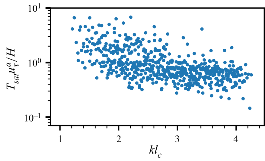
Figure 15. Distribution of saturation time  $T_{sat}$ at different wavenumbers.
5.2. Wave development in the spectral space
We analyse the properties of wave development in the spectral wavenumber space. The proposed random sweeping turbulence pressure–wave interaction model results in an explicit leading-order approximation of surface elevation variance in the principal stage of the Phillips theory (see (4.35)). The expected value of the wave energy spectrum grows linearly with time,
 \begin{align} \mathbb{E}[\hat\varPsi_{\eta}]_{{Present}}(\boldsymbol k,t)=\frac{\sqrt{2{\rm \pi}}k^{2}\hat \varPi_p(\boldsymbol k,0)t}{4\rho^{w2}\varLambda^{2} |\boldsymbol k \boldsymbol{\cdot} \boldsymbol V|}\left(\exp\left(-\frac{(\boldsymbol k \boldsymbol{\cdot} \boldsymbol U - \varLambda)^{2}}{2 (\boldsymbol k \boldsymbol{\cdot} \boldsymbol V)^{2}}\right) + \exp\left(-\frac{(\boldsymbol k \boldsymbol{\cdot} \boldsymbol U + \varLambda)^{2}}{2(\boldsymbol k \boldsymbol{\cdot} \boldsymbol V)^{2}}\right)\right),\end{align}
where the subscript ‘ ${Present}$’ denotes the present random sweeping turbulence pressure–wave interaction model. In Phillips (Reference Phillips1957), the growth of the wave energy spectrum, denoted as $\mathbb {E}[\hat \varPsi _{\eta }]_{{Phillips}}(\boldsymbol k,t)$, has the following expression:
 \begin{equation} \mathbb{E}[\hat\varPsi]_{{Phillips}}(\boldsymbol k,t)=\frac{\hat \varPi_p(\boldsymbol k,0)t}{2\sqrt{2}\rho^{w2}U_{p}g}.\end{equation}
We note that (5.3) represents a quantitative prediction of wave growth by setting the prefactor in (1.1) to be  $1$ (see Phillips Reference Phillips1957, § 4.3). We refer to (5.3) as the ‘Phillips model’.
In the Phillips theory, the shape of the wave energy spectrum is identical to the pressure energy spectrum (see (5.3)), and there is no preferred selection of energy amplifications related to the dispersion of surface waves. Our present random sweeping turbulence pressure–wave interaction model indicates a preferred amplification of the wave-growth rate near the resonance curve  $\varLambda -\boldsymbol k \boldsymbol {\cdot } \boldsymbol U=0$ because the exponential decay in (5.2) is much faster than the power-law decay.
To numerically evaluate the wave growth in the spectral space, we define the following  $L_t^{ 1}$ norm for the pressure energy spectrum $\hat \varPsi _{p}$ and the time-dependent $X_t^{ 1}$ norm for the wave energy spectrum $\hat \varPsi _{\eta }(\boldsymbol k)$:
 $$\begin{gather} \Vert\hat\varPsi_{p}(\boldsymbol k)\Vert_{L_t^{ 1}(\mathcal{T})} = \int_\mathcal{T}\hat\varPsi_{p}(\boldsymbol k, t)\, {{\rm d}}t, \end{gather}$$
 $$\begin{gather}\Vert\hat\varPsi_{\eta}(\boldsymbol k)\Vert_{X_t^{ 1}(\mathcal{T})} = \int_\mathcal{T} t^{{-}1}\hat\varPsi_{\eta}(\boldsymbol k, t)\, {{\rm d}}t, \end{gather}$$
where  $\mathcal {T}$ denotes the time interval. We note that the $X_t^{ 1}$ norm is well defined in any time interval $[0,T_M]$ because the wave energy spectrum has a power-law growth near $t=0$ (see figure 4c), and the integrand $t^{-1}\hat \varPsi _{\eta }$ is regular for any $t\in [0,T_M]$. The weighted norm $X_t^{ 1}$ captures the linear-growth behaviour of the wave energy spectrum in the principal stage and provides a direct measure to evaluate the wave growth in the spectral wavenumber space. Figure 16 shows a comparison of the $X_t^{ 1}$ norm of the wave energy spectrum among the DNS results, the present model and the Phillips model for both gravity–capillary waves and gravity waves. A total of 34 488 snapshots with a sampling interval $5.8\times 10^{-4}H/u_\tau ^{a}$ are used to generate these plots, and the time interval $\mathcal {T}$ is set to be $\mathcal {T}=[0,20H/u_\tau ^{a}]$.


As shown in figures 16(a) and 16(b), the differences in the wave energy spectrum between gravity–capillary waves and gravity waves in the wavenumber space are distinct. Our present model (5.2) successfully captures the inhomogeneity of the wave energy spectrum for both gravity–capillary waves and gravity waves, as shown in figures 16(c) and 16(d), respectively. Compared with the DNS results, the random sweeping turbulence pressure–wave interaction model predicts the wave energy spectrum in the principal stage of the wind-wave-generation process reasonably well. In contrast, the Phillips model (see (5.3)) predicts a homogeneous wave energy spectrum (figures 16e and 16f), which is identical to the pressure energy spectrum. The shape of the wave energy spectrum in the Phillips model deviates from the DNS results. Phillips (Reference Phillips1957) conjectured that in the principal stage, the resonance mechanism is insignificant, i.e.  $\varLambda \ll \boldsymbol k \boldsymbol {\cdot } \boldsymbol U$, and the temporal growth behaviour of the wave energy component is the same at all wavenumbers. Our DNS results indicate that the resonance mechanism is also essential in the principal stage, which results in the formation of different wave energy spectra for gravity–capillary waves and gravity waves. To further illustrate the significance of the resonance mechanism on the formation of the wave energy spectrum in the principal stage of the wind-wave-generation process, we calculate the ratio between the $X_t^{ 1}$ norm of the wave energy spectrum and the $L_t^{ 1}$ norm of the pressure fluctuation spectrum, i.e.
 \begin{align} \frac{\Vert\hat\varPsi_{\eta}(\boldsymbol k)\Vert_{X_t^{ 1}}}{\Vert\hat\varPsi_{p}(\boldsymbol k)\Vert_{L_t^{ 1}}}=\frac{\sqrt{2{\rm \pi}}k^{2}}{4\rho^{w2}\varLambda^{2} |\boldsymbol k \boldsymbol{\cdot} \boldsymbol V|}\left(\exp\left(-\frac{(\boldsymbol k \boldsymbol{\cdot} \boldsymbol U - \varLambda)^{2}}{2 (\boldsymbol k \boldsymbol{\cdot} \boldsymbol V)^{2}}\right) + \exp\left(-\frac{(\boldsymbol k \boldsymbol{\cdot} \boldsymbol U+\varLambda)^{2}}{2(\boldsymbol k \boldsymbol{\cdot} \boldsymbol V)^{2}}\right)\right).\end{align}
 From (5.6), we observe that the profile of  $\Vert \hat \varPsi _{\eta }(\boldsymbol k)\Vert _{X_t^{ 1}}\big /\Vert \hat \varPsi _{p}(\boldsymbol k)\Vert _{L_t^{ 1}}$ is dominated by the product of the coefficient term $k^{2}\varLambda ^{-2}|\boldsymbol k\boldsymbol {\cdot }\boldsymbol V|^{-1}$ and the Gaussian function $\exp (-(\boldsymbol k \boldsymbol {\cdot } \boldsymbol U-\varLambda )^{2}/(\boldsymbol k \boldsymbol {\cdot }\boldsymbol V)^{2})$. The coefficient term can be viewed as a power-law function with respect to the wavenumber $\boldsymbol k$. Because the decay of a Gaussian function is significantly faster than the decay of a power-law function, the profile of (5.6) can be characterised by the behaviour of resonance curve $\varLambda -\boldsymbol k \boldsymbol {\cdot } \boldsymbol U=0$ as follows. The amplitude of $k^{2}\varLambda ^{-2}|\boldsymbol k \boldsymbol {\cdot } \boldsymbol V|^{-1}$ changes slightly with the coefficient term when the wavenumber $\boldsymbol k$ moves along with the resonance curve but decays rapidly when the wavenumber $k$ moves away from the resonance curve. For gravity–capillary waves, the dispersion $\varLambda (\boldsymbol k)$ grows asymptotically as $k^{3/2}$ for large $k$, and thus, the coefficient term $k^{2}\varLambda ^{-2}|\boldsymbol k \boldsymbol {\cdot } \boldsymbol V|^{-1}$ decays asymptotically as $k^{-1}|\boldsymbol k\boldsymbol {\cdot } \boldsymbol V|^{-1}$. For gravity waves, the dispersion $\varLambda (\boldsymbol k)$ decays asymptotically as $k^{-1/2}$ for large $k$, which results in the asymptotic behaviour of the coefficient term as $k|\boldsymbol k\boldsymbol {\cdot } \boldsymbol V|^{-1}$. Therefore, we conclude that along the resonance curve, the amplitude of $\Vert \hat \varPsi _{\eta }(\boldsymbol k)\Vert _{X_t^{ 1}}/\Vert \hat \varPsi _{p}(\boldsymbol k)\Vert _{L_t^{ 1}}$ decays as $k^{-2}$ for gravity–capillary waves and does not decay along with the resonance curve for gravity waves.
To verify the above analysis, we plot the profiles of  $\Vert \hat \varPsi _{\eta }(\boldsymbol k)\Vert _{X_t^{ 1}}\big /\Vert \hat \varPsi _{p}(\boldsymbol k)\Vert _{L_t^{ 1}}$ at the wavenumber space for both gravity–capillary waves and gravity waves in figure 17. The red dashed lines represent the resonance curves $\varLambda -\boldsymbol k\boldsymbol {\cdot }\boldsymbol U=0$ for gravity–capillary waves and gravity waves. From the DNS results, we observe that the amplitude of $\Vert \hat \varPsi _{\eta }(\boldsymbol k)\Vert _{X_t^{ 1}}\big /\Vert \hat \varPsi _{p}(\boldsymbol k)\Vert _{L_t^{ 1}}$ decays fast along with the resonance curve for gravity waves (see figure 17a). However, no obvious decay along with the resonance curve can be found for gravity waves (see figure 17b). Figures 17(c) and 17(d) visualise (5.6) for gravity–capillary waves and gravity waves, respectively. Our proposed random sweeping turbulence pressure–wave interaction model shows good agreement with the DNS results. Next, we investigate the wavenumber–frequency wave spectrum $\tilde {\varPi }_\eta (\boldsymbol k,\omega )$ at different wind-wave development stages. We note that in the present wind-wave-generation problem, surface elevation $\eta (\boldsymbol x,t)$ is only defined in a space–time domain $R^{2}\times [0,\infty ]$ rather than the entirespace–time $R^{2+1}$. Nevertheless, the space–time Fourier transform can be utilised to study the dispersive properties of surface elevations under a mild assumption of artificial periodical extension in time. Take the space–time Fourier transform in (4.3), we obtain the linearised governing equation for the surface elevation $\tilde {\eta }(\boldsymbol k,\omega )$ in the wavenumber–frequency space
 \begin{equation} -\omega^{2}\tilde{\eta}+\varLambda^{2}\tilde{\eta}={-}\frac{k}{\rho^{w}}\tilde{p}. \end{equation}
Figure 17. Comparisons of  $\Vert \hat \varPsi _{\eta }(\boldsymbol k)\Vert _{X_t^{ 1}}\big /\Vert \hat \varPsi _{p}(\boldsymbol k)\Vert _{L_t^{ 1}}$ between the DNS results and the present model for gravity–capillary waves and gravity waves. The red dashed line represents the resonance curve, $\boldsymbol k \boldsymbol {\cdot } \boldsymbol U-\varLambda =0$.
The solution to  $\tilde {\eta }(\boldsymbol k,\omega )$ is given in the sense of distributions (see Tao Reference Tao2006)
 \begin{equation} \tilde{\eta}(\boldsymbol k,\omega)=\delta(|\omega|-|\varLambda(\boldsymbol k)|)\left(\frac{1}{2}\hat{\eta}_0(\boldsymbol k)-\frac{\mathrm{sgn}(\omega)}{2\,\mathrm{i}\varLambda(\boldsymbol k)}\hat{\eta}_1(\boldsymbol k)\right)+\frac{k\tilde{p}(\boldsymbol k,\boldsymbol \omega)}{\rho^{w}(\omega^{2}-\varLambda(\boldsymbol k)^{2})},\end{equation}
where  $\delta (x)$ and $\mathrm {sgn}(x)$ denote the Dirac delta function and the sign function, respectively. Here, $\eta _0$ and $\eta _1$ are the surface elevation and its temporal derivative at $t=0$, i.e. $\eta _0=\eta |_{t=0}$ and $\eta _1=\partial _t\eta |_{t=0}$. The first term on the right-hand side (right-hand side) of (5.8) represents the evolution of free surface waves subject to the initial condition at $t=0$, and the second term in right-hand side of (5.8) represents the evolution of surface waves subject to the external pressure forcing. Singularities in (5.8) can be regularised by further considering the viscosity effect (see Perrard et al. Reference Perrard, Lozano-Durán, Rabaud, Benzaquen and Moisy2019). From (5.8), because the wavenumber–frequency spectrum of pressure fluctuations $\tilde {p}$ is a continuous and bounded function of $\boldsymbol k$ and $\omega$, we can see that $|\tilde \eta |$ is concentrated near the dispersion isosurface $|\omega |-|\varLambda (\boldsymbol k)|=0$ in the sense of distributions.
Because the airflow propagates in the streamwise  $+x$-direction, we focus on the spanwise-averaged wavenumber–frequency spectrum $S_\eta (k_x,\omega )=\langle \tilde {\varPi }_\eta (\boldsymbol k,\omega )\rangle _y$ for clarity. In the spanwise-averaged wavenumber–frequency wave spectrum $S_\eta (k_x,\omega )$, the energy is concentrated in the subdomain $\mathcal {D}=\{(k_x,\omega )\mid |\omega |>\varLambda (k_x,k_y=0)\}$ because $|\boldsymbol k|\geq |k_x|$ always holds for any $\boldsymbol k=(k_x,k_y)$. Figures 18(a)–18(c) show the spanwise-averaged wavenumber–frequency wave spectrum $S_\eta (k_x,\omega )$ in the principal stage ( $0< t u_\tau ^{a}/H<20$), the transition stage ( $25< t u_\tau ^{a}/H<45$) and the exponential growth stage ( $50< t u_\tau ^{a}/H<70$), respectively. In each stage, a total of 8 622 consecutive snapshots with a sampling interval $2.3\times 10^{-3}H/u_\tau ^{a}$ are collected for conducting space–time Fourier transform. The red dashed lines denote the dispersion curve $\omega =\varLambda (k_x,k_y=0)$, representing the boundaries of domain $\mathcal {D}$. As shown in figure 18, most of the energy of $S_\eta$ is concentrated inside $\mathcal {D}$, which is consistent with the above theoretical analysis and is similar to the wavenumber–frequency spectrum of viscous wrinkles studied by Perrard et al. (Reference Perrard, Lozano-Durán, Rabaud, Benzaquen and Moisy2019). Specifically, the oblique stripe structures in figure 18 reveal the dispersion relations subject to discrete values of $k_y$ in numerical simulations. For example, an orange curve in figure 18(a) illustrates a dispersion relation $\omega =\varLambda (k_x, k_y)$ with the discrete value of $k_yl_c=0.56$ being the fifth smallest non-zero wavenumber in the $k_y$-direction. The orange curve coincides with the corresponding strip structure in the spectrum, which indicates that the spanwise-averaged wavenumber–frequency spectrum $S(k_x,\omega )$ reveals the dispersion properties of surface elevations in the two-dimensional wavenumber space.
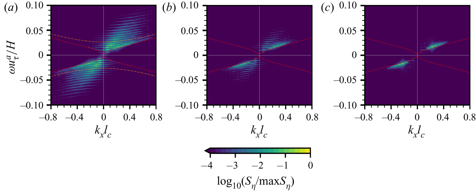
Figure 18. The space–frequency spectrum of surface elevation  $S_\eta$, normalised by its maximum value, in (a) the principal stage, i.e. $0< t u_\tau ^{a}/H<20$, (b) the transition stage, i.e. $25< t u_\tau ^{a}/H<45$ and (c) the exponential growth stage, i.e. $50< t u_\tau ^{a}/H<70$. Red dashed lines denote the dispersion curve $\omega =\pm \varLambda (\boldsymbol k)$ when $k_y=0$. Orange dashed lines in (a) denote the dispersion curve $\omega =\pm \varLambda (\boldsymbol k)$ when the discrete value of $k_y$ satisfies $k_yl_c=0.56$.
As shown in the second term on the right-hand side of (5.8), the role of turbulent pressure fluctuations is to excite surface elevations at broadband wavenumbers and to modulate their relative strength among different wavenumbers. In (5.8),  $\tilde {\eta }$ is singular on the dispersion isosurface $|\omega |=|\varLambda (\boldsymbol k)|$, but away from the dispersion isosurface, $\tilde {\eta }$ still has non-zero finite value. It indicates that the majority of energy in the surface elevation spectrum obeys the dispersion relation of surface waves in the wavenumber–frequency space. The energy is concentrated over a wide range of $k_y$, as shown in figure 18(a), indicating that the small-scale surface deformations are generated in the principal stage. Figure 18(b) shows the wavenumber–frequency spectrum in the transition stage between the Phillips theory and the Miles theory. The majority of energy moves towards the dispersion curve where $k_y=0$. Figure 18(c) shows $S_\eta (k_x,\omega )$ in the late phase where the surface elevation variance grows exponentially in time. Most energy in the spectrum is concentrated near the dispersion curve where $k_y=0$, indicating the onset of streamwise dominant regular waves.
5.3. Further discussion on the present model for wave growth in the physical space
The expected value of surface elevation variance  $\mathbb {E}[\langle \eta ^{2}\rangle ](t)$ is related to the expected value of the wave energy spectrum $\mathbb {E}[\hat \varPsi ](\boldsymbol k,t)$ via the inverse Fourier transform (see (4.17)). The present random sweeping turbulence pressure–wave interaction model has two independent parameters, the convection velocity vector $\boldsymbol U$ and the sweeping velocity vector $\boldsymbol V$ of the air pressure fluctuations at the water surface, to quantitatively describe the wave-growth behaviour in both the wavenumber space and the physical space. As shown in figures 8(a) and 8(b), both the convection velocity and sweeping velocity are functions of wavenumber, the information of which is needed in the direct integration of (4.17). We recognise that the convection and sweeping velocities of air pressure fluctuations in wall-bounded turbulent flows are open research questions (see He et al. Reference He, Jin and Yang2017). There have not yet been satisfying closed forms developed for the $\boldsymbol U$ and $\boldsymbol V$ of pressure fluctuations yet, and this is beyond the scope of the present paper. Nevertheless, we can perform the following analyses on the range of our new model, which shows more accurate predictions than the Phillips model.
From the plots of  $U_{p}$ and $V_{p}$ against wavenumber $k_x$ in the wavenumber space (see figures 8a and 8b), we observe that $U_{p}$ varies within the interval $U_{p}\in [12.2u_\tau ^{a},16.2u_\tau ^{a}]$ and $V_{p}$ varies within the interval $V_{p}\in [3.1u_\tau ^{a},3.5u_\tau ^{a}]$ for the wavenumbers $k_xl_c\leq 0.6$. Therefore, we consider the vector $\boldsymbol q=(q_1,q_2)=(U_{p}, V_{p})$ that is located within a continuous two-dimensional parameter space $\mathcal {Q}$, defined as the following direct product:
 \begin{equation} \mathcal{Q}=[12.2u_\tau^{a},16.2u_\tau^{a}]\times[3.1u_\tau^{a},3.5u_\tau^{a}]. \end{equation}
Using our new model (5.2), we estimate the expected value of surface elevation variance in the physical space by computing
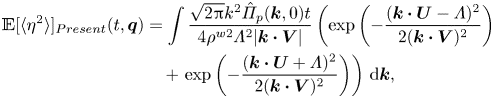 \begin{align} \mathbb{E}[\langle\eta^{2}\rangle]_{{Present}}(t,\boldsymbol q)&=\int \frac{\sqrt{2{\rm \pi}}k^{2}\hat \varPi_p(\boldsymbol k,0)t}{4\rho^{w2}\varLambda^{2} |\boldsymbol k \boldsymbol{\cdot} \boldsymbol V|}\left(\exp\left(-\frac{(\boldsymbol k \boldsymbol{\cdot} \boldsymbol U - \varLambda)^{2}}{2 (\boldsymbol k \boldsymbol{\cdot} \boldsymbol V)^{2}}\right) \right.\nonumber\\ &\quad + \left.\exp\left(-\frac{(\boldsymbol k \boldsymbol{\cdot} \boldsymbol U + \varLambda)^{2}}{2(\boldsymbol k \boldsymbol{\cdot} \boldsymbol V)^{2}}\right)\right)\, \mathrm{d}\boldsymbol k, \end{align}
where the constants  $\boldsymbol U$ and $\boldsymbol V$ are related to the vector $\boldsymbol q$ through $\boldsymbol U=(q_1,0)$ and $\boldsymbol V=(q_2,0)$, respectively. As a result, the expected value of surface elevation variance $\mathbb {E}[\langle \eta ^{2}\rangle ]_{{Present}}$ in the present model is a continuous function of the vector $\boldsymbol q\in \mathcal {Q}$. We calculate the upper bound and the lower bound of $\mathbb {E}[\langle \eta ^{2}\rangle ]_{{Present}}$ with respect to $q$ to obtain an estimation of the expected value of surface elevation variance $\mathbb {E}[\langle \eta ^{2}\rangle ](t)$,
 \begin{equation} \min_{\boldsymbol q\in\mathcal{Q}} \mathbb{E}[\langle\eta^{2}\rangle]_{{Present}}(\boldsymbol q,t)\leq \mathbb{E}[\langle\eta^{2}\rangle](t) \leq \max_{\boldsymbol q\in\mathcal{Q}} \mathbb{E}[\langle\eta^{2}\rangle]_{{Present}}(\boldsymbol q,t).\end{equation}
 The estimation (5.11) results in the growth rate of surface elevation variance  $\mathbb {E}[\langle \eta ^{2}\rangle ](t)$ that is within a certain range. We note that in the present model, the prediction of the linear wave-growth rate only requires the spatial Fourier transform of surface turbulence pressure fluctuations. As shown in (4.15), wave growth is closely related to the spatial-temporal evolution of turbulence pressure fluctuations. The present model reduces the cost of computing the wavenumber–frequency spectrum to the wavenumber spectrum by assuming the random sweeping hypothesis. The Phillips model neglects the resonance mechanism in the principal stage, and predicts that the wave-growth rate in the physical space is proportional to an unweighted integral of the pressure fluctuation energy spectrum which is equivalent to the mean square of surface pressure fluctuations. Our model further takes into account the effects of the resonance mechanism in the principal stage, and the computation of the wave-growth rate can be viewed as a weighted integral of the pressure fluctuation energy spectrum. Figure 19 compares surface elevation variance among the DNS results, the present model (see (5.10)) and the Phillips model (see (1.1)) for both gravity–capillary waves and gravity waves in the principal stage of wave development. In the Phillips model, the surface elevation variance is related to the convection velocity $U_{p}$. We use the same methodology as above in which the convection velocity varies in a certain range, i.e. $U_{p}\in [12.2 u_\tau ^{a},16.2 u_\tau ^{a}]$, to obtain that the Phillips model also provides a wave-growth prediction with finite bandwidth. Because the Phillips model neglects the surface tension effect, it results in identical expressions of surface elevation variance for gravity–capillary waves and gravity waves. As shown in figure 19, the Phillips model underestimates the growth of surface elevation variance for both gravity–capillary waves and gravity waves, which is consistent with the finding from the previous numerical simulations by Lin et al. (Reference Lin, Moeng, Tsai, Sullivan and Belcher2008). In contrast, the present model has much better agreement with the DNS results for both gravity–capillary waves and gravity waves. In the early phase when $tu_\tau ^{a}/H\leq 4$, figures 19(a) and 19(b) show that most DNS wave fluctuation data $\langle \eta ^{2}\rangle /H^{2}$ are located within the shaded range predicted by the present model. In the entire principal stage $tu_\tau ^{a}/H\leq 20$ (see figure 19c), the DNS results match well with the present model for gravity–capillary waves. For gravity waves, figure 19(d) shows that the present model overpredicts the wave growth for gravity waves. Note that the linear-growth rate in the DNS results for gravity waves has a slight decrease when $tu_\tau ^{a}/H>4$, which results in the deviation between DNS and the present model. The mechanisms of the change in the wave-growth rate for gravity waves need further research. Nevertheless, for gravity–capillary waves, the present model can quantitatively predict the linear growth of surface elevation variance and shows good agreement with DNS (figure 19c). We note that in the wind-wave-generation problem, waves are generated from an initially calm water surface, and the small-scale deformation of the air–water interface dominates the wave dynamics in the early phases of wind–wave development. The surface tension effect plays a key role in the evolution of water waves with short wavelengths. Therefore, compared with gravity waves, modelling the growth of gravity–capillary waves is more relevant for the present research focus on the early stage.
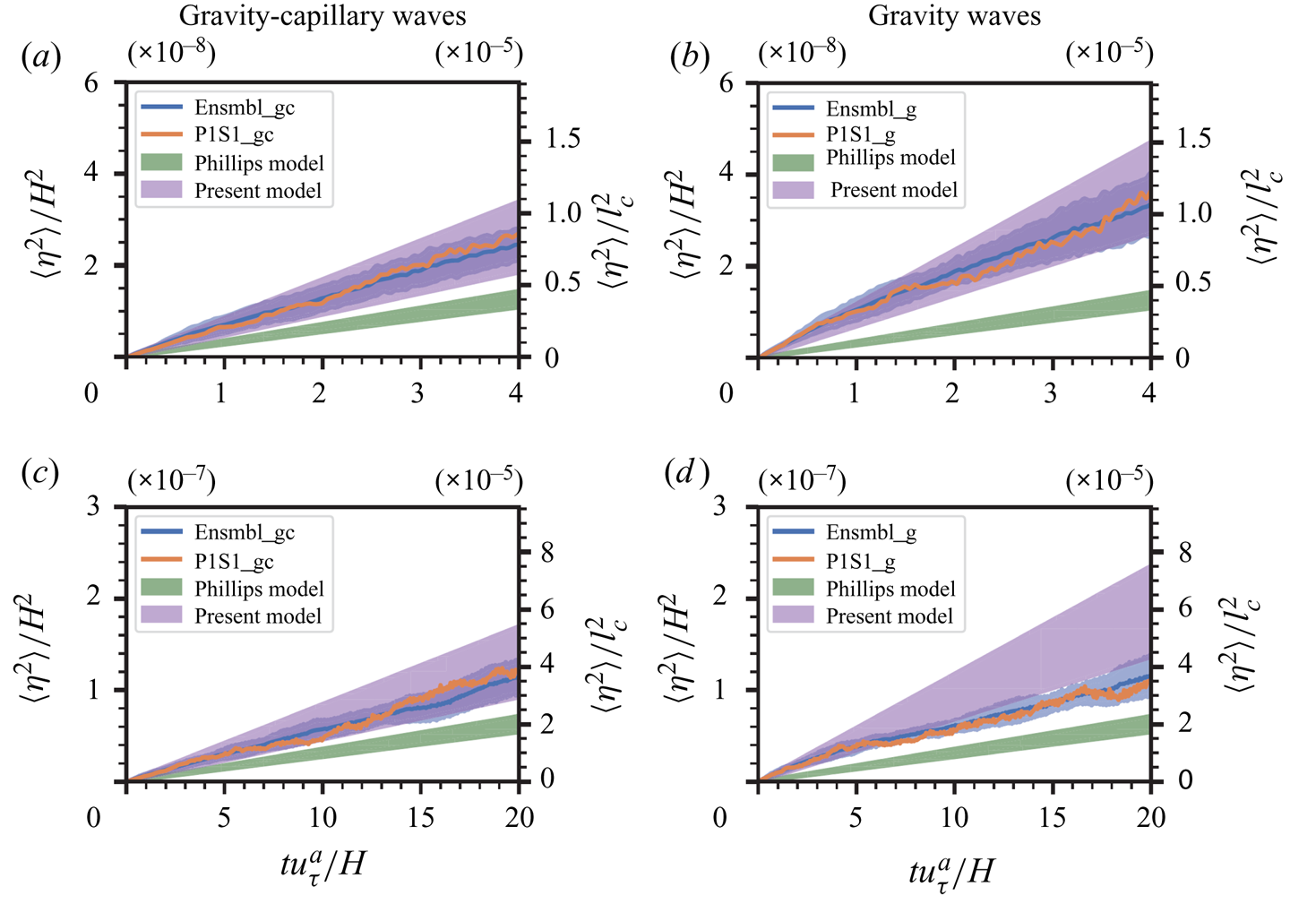
Figure 19. Comparisons of wave growth in the principal stage among the DNS results, the present model and the Phillips model for (a) gravity–capillary waves and (b) gravity waves. The orange lines represent the superresolution cases (Group II). The blue lines denote the average of the ensemble cases (Group I), with the light blue shaded area being the range bounded by one standard deviation of the ensemble data. The purple and green shaded areas show the surface elevation variance predictions by the present model and the Phillips model, respectively.
We note that Perrard et al. (Reference Perrard, Lozano-Durán, Rabaud, Benzaquen and Moisy2019) investigated the dynamics of wrinkles in a viscous fluid and proposed a spectral theory for the spatial-temporal evolution of wrinkles in a statistically steady state. The authors introduced the viscous effect of liquid to the evolution equation of water waves subject to turbulent pressure forcing and derived the spectrum of surface elevation in a statistically steady state by considering the balance between viscous dissipation and turbulent air input. They conducted synthetic wrinkles simulations to reproduce the previous experimental observations by Paquier et al. (Reference Paquier, Moisy and Rabaud2015) and Paquier et al. (Reference Paquier, Moisy and Rabaud2016). In the present study, we numerically investigate the early stage of wind-wave generation using a coupled air–water simulation solver. We systematically evaluate the Phillips theory by examining wave-growth behaviour in both the physical space and wavenumber space. A random sweeping hypothesis is introduced to model the wavenumber–frequency spectrum of turbulent pressure fluctuations. By combining the random sweeping model and linear water wave equation, we propose a closure model to predict the wave-growth rate in the principal stage and analytically obtain an asymptotic solution for the expected value of surface elevation variance.
6. Conclusions
In this work, we conduct a systematic study on the profound and long-standing problem of wind-wave generation with a focus on its early stage. Using a combined theoretical and simulation-assisted approach, we revisit the classic work by Phillips (Reference Phillips1957). Phillips conjectured that there exists a principal stage when waves grow linearly with time. We conducted high-resolution DNSs to study wave development when turbulent airflow blows over an initially flat water surface. Ensemble cases and superresolution cases for both gravity–capillary waves and gravity waves are run to elucidate the temporal behaviour of wave growth and the role of surface tension on the formation of the wave energy spectrum. The total computational cost is over  $2\times 10^{7}$ CPU hours on a high performance parallel supercomputer. The simulations capture the multistage evolution of water waves under wind forcing during the early phase of the wind-wave generation process. Initially, the air–water interface is distorted by the convection of the turbulent pressure and stress fluctuations of airflow, and the surface elevation variance grows linearly with time in the principal stage predicted by Phillips (Reference Phillips1957). In the late stage, the wave grows exponentially with time due to the shear flow instability mechanism first proposed by Miles (Reference Miles1957). Through a rigorous analysis, we confirm the existence of the principal stage when the elapsed time does not exceed $20H/u_\tau ^{a}$. We also observe the oscillation of surface elevation variance via high-frequency data sampling. The oscillation is further substantiated theoretically by asymptotic analysis.
We develop a theoretical framework of the closure model for wave generation in the principal stage of the Phillips theory. A random sweeping turbulence pressure–wave interaction model is developed to quantitatively describe the wave dynamics in the wavenumber space and physical space during the principal stage in the Phillips theory. The present model uses a combination of Taylor's frozen hypothesis and random sweeping hypothesis to model the evolution of air turbulent pressure fluctuations exerted on the air–water interface, which is inspired by the works of He & Zhang (Reference He and Zhang2006) and Wilczek & Narita (Reference Wilczek and Narita2012). A stochastic closure evolution equation for the wave elevation is derived. Different from the Phillips model, where the scaling coefficient is determined approximately, the proposed model quantitatively describes the wave evolution. Based on the analytical solution to the present model, we conduct a rigorous asymptotic analysis on the expected value of wave energy components and obtain the first three leading-order terms, which are a linear function of time, a trigonometric oscillation function of time and a constant, respectively. By comparing the relative strength among these leading-order terms, we further find that even though the amplitude of the linear-growth term is larger than the oscillating term in the principal stage, their instantaneous growth rate can be comparable. This result explains the oscillation phenomenon of temporal wave fluctuation growth observed from our DNS results in physical space and is further validated by analysing the wave energy spectrum in wavenumber space.
We use a time-dependent norm to quantify the growth behaviour of each wave energy component and compare the DNS results with the present model and the Phillips model. The Phillips model yields that the distribution of the wave energy spectrum is identical to the pressure energy spectrum. Both the DNS results and the present model reveal the inhomogeneity in the wavenumber space, and they have good agreement with each other. The present model elucidates the role of the resonance mechanism on the formation of the wave energy spectrum in the principal stage of the wind-wave-generation process. The resonance curves are distinct in the wavenumber space. Gravity–capillary waves and gravity waves have different dispersion relationships, which leads to differences in the distributions of wave energy spectra. Based on the present model, we obtain an estimation of the linear-growth rate of surface elevation variance in the principal stage of the wind-wave-generation process. We provide an expression of the upper bound and the lower bound of the expected value of surface elevation variance. While the Phillips model underestimates the wave-growth rate, the present model provides a much more accurate estimation that has good agreement with DNS data of gravity–capillary waves.
Supplementary materials
Supplementary materials are available at https://doi.org/10.1017/jfm.2021.1153.
Acknowledgements
The authors would like to thank the three anonymous reviewers for their helpful comments and suggestions. L.S. gratefully acknowledges the continuous support of the Office of Naval Research on this profound research topic of great significance in basic research.
Declaration of interests
The authors report no conflict of interest.
Appendix A. Numerical method
A.1. Grid transformation
The lower boundary of the air domain  $\varOmega ^{a}$ and the upper boundary of the water domain $\varOmega ^{w}$ are the dynamically evolving water surface. We adopt the following algebraic mapping to transform each irregular physical domain $(x,y,z,t)$ into a rectangular computational domain $(\xi,\varphi,\zeta,\tau )$:
 $$\begin{gather} \xi^{a}=x^{a}, \quad \varphi^{a}=y^{a},\quad \zeta^{a}=\frac{z-\eta(x,y,t)}{-\eta(x,y,t)+{H^{a}}}, \quad \tau^{a} =t^{a}\quad \text{in }\varOmega^{a}, \end{gather}$$
 $$\begin{gather}\xi^{w}=x^{w}, \quad \varphi^{w}=y^{w},\quad \zeta^{w}=\frac{z+H^{w}}{\eta(x,y,t)+H^{w}}, \quad \tau^{w}=t^{w}\quad \text{in }\varOmega^{w}. \end{gather}$$
The corresponding Jacobian matrices  $\boldsymbol J^{a}$ and $\boldsymbol J^{w}$ are
 \begin{align} \boldsymbol J^{a}&= \left[ \begin{array}{cccc} \xi^{a}_x & \xi^{a}_y & \xi^{a}_z & \xi^{a}_t\\ \varphi^{a}_ x & \varphi^{a}_y & \varphi^{a}_z & \varphi^{a}_t\\ \zeta^{a}_x & \zeta^{a}_y & \zeta^{a}_z & \zeta^{a}_t\\ \tau^{a}_x & \tau^{a}_y & \tau^{a}_z & \tau^{a}_t \end{array} \right] \nonumber\\ &=\left[ \begin{array}{cccc} 1 & 0 & 0 & 0\\0 & 1 & 0 & 0\\\dfrac{(z^{a}-H^{a})\eta_x}{(-\eta+H^{a})^{2}} & \dfrac{(z^{a}-H^{a})\eta_y}{(-\eta+H^{a})^{2}} & \dfrac{1}{-\eta+H^{a}} & \dfrac{(z^{a}-H^{a})\eta_t}{(-\eta+H^{a})^{2}}\\ 0 & 0 & 0 & 1 \end{array}\right], \end{align}
 \begin{align} \boldsymbol J^{w}&= \left[ \begin{array}{cccc} \xi^{w}_x & \xi^{w}_y & \xi^{w}_z & \xi^{w}_t\\ \varphi^{w}_ x & \varphi^{w}_y & \varphi^{w}_z & \varphi^{w}_t\\ \zeta^{w}_x & \zeta^{w}_y & \zeta^{w}_z & \zeta^{w}_t\\ \tau^{w}_x & \tau^{w}_y & \tau^{w}_z & \tau^{w}_t \end{array} \right] \nonumber\\ &=\left[ \begin{array}{cccc} 1 & 0 & 0 & 0\\0 & 1 & 0 & 0\\ \dfrac{-(z^{w}+H^{w})\eta_x}{(\eta+H^{w})^{2}} & \dfrac{-(z^{w}+H^{w})\eta_y}{(\eta+H^{w})^{2}} & \dfrac{1}{\eta+H^{w}} & \dfrac{-(z^{w}+H^{w})\eta_t}{(\eta+H^{w})^{2}}\\ 0 & 0 & 0 & 1\end{array}\right], \end{align}
where the subscripts denote partial derivatives.
Transforming equations (2.1a)–(2.1d) from the physical coordinates  $(x,y,z,t)$ to the computational coordinates $(\xi,\varphi,\zeta,\tau )$ in each domain, we obtain
 \begin{align}
&\frac{\partial u^{\epsilon}}{\partial \xi^{\epsilon}}
+\zeta^{\epsilon}_x\frac{\partial
u^{\epsilon}}{\partial\zeta^{\epsilon}} +\frac{\partial
v^{\epsilon}}{\partial
\varphi^{\epsilon}}+\zeta^{\epsilon}_y \frac{\partial
v^{\epsilon}}{\partial \zeta^{\epsilon}}+\zeta^{\epsilon}_z
\frac{\partial w^{\epsilon}}{\partial
\zeta^{\epsilon}}=0,\\ &\frac{\partial
u^{\epsilon}}{\partial\tau^{\epsilon}}+\zeta^{\epsilon}_t
\frac{\partial
u^{\epsilon}}{\partial\zeta^{\epsilon}}+\frac{\partial
(u^{\epsilon}
u^{\epsilon})}{\partial\xi^{\epsilon}}+\zeta^{\epsilon}_x
\frac{\partial(u^{\epsilon}
u^{\epsilon})}{\partial\zeta^{\epsilon}}
+\frac{\partial(u^{\epsilon} v^{\epsilon})}{\partial
\varphi^{a}}+\zeta^{\epsilon}_y \frac{\partial(u^{\epsilon}
v^{\epsilon})}{\partial\zeta^{\epsilon}}
+\zeta^{\epsilon}_z\frac{\partial(u^{\epsilon}
w^{\epsilon})}{\partial\zeta^{\epsilon}} \nonumber\\ &\quad
={-}\frac{1}{\rho^{\epsilon}}\left(\frac{\partial
p^{\epsilon}}{\partial \xi^{\epsilon}}
+\zeta^{\epsilon}_x\frac{\partial p^{a}}{\partial
\zeta^{\epsilon}}\right)
+\nu^{\epsilon}\nabla^{2}u^{\epsilon},
\end{align}
\begin{align}
&\frac{\partial u^{\epsilon}}{\partial \xi^{\epsilon}}
+\zeta^{\epsilon}_x\frac{\partial
u^{\epsilon}}{\partial\zeta^{\epsilon}} +\frac{\partial
v^{\epsilon}}{\partial
\varphi^{\epsilon}}+\zeta^{\epsilon}_y \frac{\partial
v^{\epsilon}}{\partial \zeta^{\epsilon}}+\zeta^{\epsilon}_z
\frac{\partial w^{\epsilon}}{\partial
\zeta^{\epsilon}}=0,\\ &\frac{\partial
u^{\epsilon}}{\partial\tau^{\epsilon}}+\zeta^{\epsilon}_t
\frac{\partial
u^{\epsilon}}{\partial\zeta^{\epsilon}}+\frac{\partial
(u^{\epsilon}
u^{\epsilon})}{\partial\xi^{\epsilon}}+\zeta^{\epsilon}_x
\frac{\partial(u^{\epsilon}
u^{\epsilon})}{\partial\zeta^{\epsilon}}
+\frac{\partial(u^{\epsilon} v^{\epsilon})}{\partial
\varphi^{a}}+\zeta^{\epsilon}_y \frac{\partial(u^{\epsilon}
v^{\epsilon})}{\partial\zeta^{\epsilon}}
+\zeta^{\epsilon}_z\frac{\partial(u^{\epsilon}
w^{\epsilon})}{\partial\zeta^{\epsilon}} \nonumber\\ &\quad
={-}\frac{1}{\rho^{\epsilon}}\left(\frac{\partial
p^{\epsilon}}{\partial \xi^{\epsilon}}
+\zeta^{\epsilon}_x\frac{\partial p^{a}}{\partial
\zeta^{\epsilon}}\right)
+\nu^{\epsilon}\nabla^{2}u^{\epsilon},
\end{align}
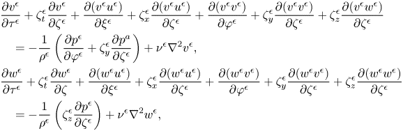 \begin{align}
&\frac{\partial v^{\epsilon}}{\partial\tau^{\epsilon}}
+\zeta^{\epsilon}_t \frac{\partial
v^{\epsilon}}{\partial\zeta^{\epsilon}}+\frac{\partial
(v^{\epsilon}
u^{\epsilon})}{\partial\xi^{\epsilon}}+\zeta^{\epsilon}_x\frac{\partial(v^{\epsilon}
u^{\epsilon})}{\partial\zeta^{\epsilon}}
+\frac{\partial(v^{\epsilon} v^{\epsilon})}{\partial
\varphi^{\epsilon}}+\zeta^{\epsilon}_y
\frac{\partial(v^{\epsilon}
v^{\epsilon})}{\partial\zeta^{\epsilon}}
+\zeta^{\epsilon}_z\frac{\partial(v^{\epsilon}
w^{\epsilon})}{\partial\zeta^{\epsilon}} \nonumber\\ &\quad
={-}\frac{1}{\rho^{\epsilon}}\left(\frac{\partial
p^{\epsilon}}{\partial \varphi^{\epsilon}}
+\zeta^{\epsilon}_y\frac{\partial p^{a}}{\partial
\zeta^{\epsilon}}\right)+\nu^{\epsilon}
\nabla^{2}v^{\epsilon},\\
&\frac{\partial w^{\epsilon}}{\partial\tau^{\epsilon}}
+\zeta^{\epsilon}_t \frac{\partial
w^{\epsilon}}{\partial\zeta}+\frac{\partial (w^{\epsilon}
u^{\epsilon})}{\partial\xi^{\epsilon}}+\zeta^{\epsilon}_x\frac{\partial(w^{\epsilon}
u^{\epsilon})}{\partial\zeta^{\epsilon}}
+\frac{\partial(w^{\epsilon} v^{\epsilon})}{\partial
\varphi^{\epsilon}}
+\zeta^{\epsilon}_y\frac{\partial(w^{\epsilon}
v^{\epsilon})}{\partial\zeta^{\epsilon}}
+\zeta^{\epsilon}_z\frac{\partial(w^{\epsilon}
w^{\epsilon})}{\partial\zeta^{\epsilon}} \nonumber\\
&\quad
={-}\frac{1}{\rho^{\epsilon}}\left(\zeta^{\epsilon}_z\frac{\partial
p^{\epsilon}}{\partial
\zeta^{\epsilon}}\right)+\nu^{\epsilon}\nabla^{2}w^{\epsilon},
\end{align}
\begin{align}
&\frac{\partial v^{\epsilon}}{\partial\tau^{\epsilon}}
+\zeta^{\epsilon}_t \frac{\partial
v^{\epsilon}}{\partial\zeta^{\epsilon}}+\frac{\partial
(v^{\epsilon}
u^{\epsilon})}{\partial\xi^{\epsilon}}+\zeta^{\epsilon}_x\frac{\partial(v^{\epsilon}
u^{\epsilon})}{\partial\zeta^{\epsilon}}
+\frac{\partial(v^{\epsilon} v^{\epsilon})}{\partial
\varphi^{\epsilon}}+\zeta^{\epsilon}_y
\frac{\partial(v^{\epsilon}
v^{\epsilon})}{\partial\zeta^{\epsilon}}
+\zeta^{\epsilon}_z\frac{\partial(v^{\epsilon}
w^{\epsilon})}{\partial\zeta^{\epsilon}} \nonumber\\ &\quad
={-}\frac{1}{\rho^{\epsilon}}\left(\frac{\partial
p^{\epsilon}}{\partial \varphi^{\epsilon}}
+\zeta^{\epsilon}_y\frac{\partial p^{a}}{\partial
\zeta^{\epsilon}}\right)+\nu^{\epsilon}
\nabla^{2}v^{\epsilon},\\
&\frac{\partial w^{\epsilon}}{\partial\tau^{\epsilon}}
+\zeta^{\epsilon}_t \frac{\partial
w^{\epsilon}}{\partial\zeta}+\frac{\partial (w^{\epsilon}
u^{\epsilon})}{\partial\xi^{\epsilon}}+\zeta^{\epsilon}_x\frac{\partial(w^{\epsilon}
u^{\epsilon})}{\partial\zeta^{\epsilon}}
+\frac{\partial(w^{\epsilon} v^{\epsilon})}{\partial
\varphi^{\epsilon}}
+\zeta^{\epsilon}_y\frac{\partial(w^{\epsilon}
v^{\epsilon})}{\partial\zeta^{\epsilon}}
+\zeta^{\epsilon}_z\frac{\partial(w^{\epsilon}
w^{\epsilon})}{\partial\zeta^{\epsilon}} \nonumber\\
&\quad
={-}\frac{1}{\rho^{\epsilon}}\left(\zeta^{\epsilon}_z\frac{\partial
p^{\epsilon}}{\partial
\zeta^{\epsilon}}\right)+\nu^{\epsilon}\nabla^{2}w^{\epsilon},
\end{align}
with the symbol  $\epsilon =\{a,w\}$ indicating variables in the air and water domains, respectively.
A.2. Boundary conditions
The horizontal boundary conditions are periodic in the  $x$- and $y$-directions. At the top boundary of the air domain, we apply a constant shear stress in the $x$ direction to simulate the shear-driven air turbulence. At the bottom of the water domain, we use the no-slip velocity boundary condition. Dirichlet boundary conditions of velocity components and the profile of wave waves are used as the bottom boundary condition for the air motion, written as
 \begin{equation} u^{a}=u^{w}, v^{a}=v^{w}, w^{a}=w^{w} \text{ at }z=\eta(x,y,t).\end{equation}
The motion of wave surface elevation  $\eta$ is governed by the kinematic boundary condition of the air–water interface,
 \begin{equation} \eta_t=w^{w}-u^{w}\eta_x-v^{w}\eta_y \text{ at } z=\eta(x,y,t).\end{equation}
For the water domain, the upper boundary conditions for velocity components and pressure are the dynamic boundary conditions on the water surface,
 $$\begin{gather} \boldsymbol{t_1}\boldsymbol{\cdot}\boldsymbol{\sigma}^{w}\boldsymbol{\cdot} \boldsymbol{n}^{\mathsf{\text{T}}}=\boldsymbol{t_1} \boldsymbol{\cdot}\boldsymbol{\sigma}^{a}\boldsymbol{\cdot} \boldsymbol{n}^{\mathsf{\text{T}}} \text{ at } z=\eta(x,y,t), \end{gather}$$
 $$\begin{gather}\boldsymbol{t_2}\boldsymbol{\cdot}\boldsymbol{\sigma}^{w}\boldsymbol{\cdot} \boldsymbol{n}^{\mathsf{\text{T}}}=\boldsymbol{t_2} \boldsymbol{\cdot}\boldsymbol{\sigma}^{a}\boldsymbol{\cdot} \boldsymbol{n}^{\mathsf{\text{T}}} \text{ at } z=\eta(x,y,t), \end{gather}$$
 $$\begin{gather}\boldsymbol{n}\boldsymbol{\cdot}\boldsymbol{\sigma}^{w}\boldsymbol{\cdot} \boldsymbol{n}^{\mathsf{\text{T}}}=\boldsymbol{n} \boldsymbol{\cdot}\boldsymbol{\sigma}^{a}\boldsymbol{\cdot} \boldsymbol{n}^{\mathsf{\text{T}}}+\Delta p \text{ at } z=\eta(x,y,t), \end{gather}$$
where the stress tensor is  $\boldsymbol \sigma _{ij}=-(p-\rho gz)\delta _{ij}+\nu (u_{i,j}+u_{j,i})$, $\boldsymbol {n}$, $\boldsymbol {t_1}$ and $\boldsymbol {t_2}$ denote the normal vectors and two tangential vectors of the air–water interface, respectively, and $\Delta p$ is the difference in normal stress across the air–water interface due to the surface tension.
A.3. Numerical algorithms
The governing equations are spatially discretised by a Fourier-based pseudospectral method in the horizontal  $(\xi,\varphi )$ plane and a second-order finite difference method in the vertical $\zeta$-direction. The $(\xi,\varphi )$ plane uses an evenly spaced mesh. Grid points in the vertical $\zeta$-direction are clustered near the upper and lower boundaries of the air and water domains. The governing equations (A4a)–(A4b) in the computational air and water domains are solved using a fractional-step method (Kim & Moin Reference Kim and Moin1985). A second-order Adams–Bashforth scheme is applied to the convection terms, and the viscous terms and the $\zeta _t$-related terms are discretised using the Crank–Nicholson scheme. The evolution equation of the air–water interface elevation in (A6) is calculated using a predictor–corrector method fully coupled with the Navier–Stokes equation solver. An iteration scheme is used to satisfy the continuation of velocity (A5) and constraints of stress tensors (A7) at the air–water interface. Details of the numerical schemes are provided in Yang & Shen (Reference Yang and Shen2011a,Reference Yang and Shenb) and Xuan & Shen (Reference Xuan and Shen2019). Applications of our numerical method to various turbulence–wave interaction problems can be found in Yang & Shen (Reference Yang and Shen2010), Yang et al. (Reference Yang, Meneveau and Shen2013), Yang et al. (Reference Yang, Meneveau and Shen2014a,Reference Yang, Meneveau and Shenb), Hao & Shen (Reference Hao and Shen2019), Xuan & Shen (Reference Xuan and Shen2019), Xuan et al. (Reference Xuan, Deng and Shen2020), Cao et al. (Reference Cao, Deng and Shen2020) and Cao & Shen (Reference Cao and Shen2021).
Appendix B. Individual realisations of ensemble simulations
In this appendix, we visualise individual realisations of ensemble simulations (Group I). Figure 20 shows the temporal growth behaviours of surface elevation variance  $\langle \eta ^{2}\rangle$ in the wind-wave-generation process. The early development of surface waves interacting with turbulent airflow is an unsteady problem, and thus variations among different independent simulations are expected. We use coefficient of variation (CV), i.e. the ratio between the standard deviation and the mean, to quantify the variations among different realisations. As illustrated in figures 20(a) and 20(b), surface elevation variance $\langle \eta ^{2}\rangle$ grows linearly with time in the early phase when $tu_\tau ^{a}/H<20$. The averaged CV of surface elevation variance $\langle \eta ^{2}\rangle$ in the time interval $t u_\tau ^{a}/H\in [0,20]$ is $16\,\%$ and $13\,\%$ for gravity–capillary waves and gravity waves, respectively. Figures 20(c) and 20(d) show the exponential growth behaviour of $\langle \eta ^{2}\rangle$ in the late phase when $tu_\tau ^{a}/H>50$. The exponential growth rate of surface elevation variance (i.e. the slope in figures 20c and 20d) is closely related to Miles’ critical-layer theory. We extract the exponential growth rate in each individual simulation during the time interval $t u_\tau ^{a}/H\in [50,75]$ using the least squares method. The CV of the exponential growth rate is $1\,\%$, which indicates that all individual realisations exhibit a consistent exponential growth rate in the late phase.

Figure 20. Individual realisations of the temporal growth of surface elevation variance  $\langle \eta ^{2}\rangle$ in the ensemble simulations of gravity–capillary waves and gravity waves. Surface elevation variance $\langle \eta ^{2}\rangle$ is normalised by the air domain height $H$ and the capillary length scale $l_c$, shown on the left and right $y$-axes, respectively. The dashed line (– –, blue) denotes each individual realisation, the solid line (——, orange) denotes the ensemble average. Panels (a) and (b) show the linear temporal growth behaviour in the early stage, with the $y$-axis plotted in linear scale; (c) and (d) show the exponential temporal growth behaviour in the late stage, with the $y$-axis plotted in logarithmic scale.
Appendix C. Diagnostic functions of linear-growth behaviour
We examine the existence of the principal stage of wave development (Phillips Reference Phillips1957) in the physical space. To validate that there exists a certain time period within which the surface elevation variance  $\langle \eta ^{2}\rangle$ grows linearly with time, we adopt its first- and second-order time derivatives as the diagnostic functions. If the hypothesis of the principal stage holds, the first derivative and second derivative of the surface elevation variance should be constant and zero, respectively. We sample the surface wave elevation $\eta (x,y)$ every $1.44\times 10^{2}H/u_\tau ^{a}$ and collect 2778 consecutive snapshots for each realisation in case Ensembl_gc. The ensemble average of surface elevation variance $\mathbb {E}[\langle \eta ^{2}\rangle ]$, which is a discrete function of time instant $t$, is then computed based on these data
 \begin{equation} \mathbb{E}[\langle\eta^{2}\rangle](t)=\frac{1}{N_e N_x N_y}\sum_k^{N_e}\sum_i^{N_x}\sum_j^{N_y} \eta^{2}_{(k)}(x_i,y_j,t). \end{equation}
Here,  $\eta _{(k)}(x_i,y_j,t)$ denotes the surface elevation at grid point $(x_i,y_j)$ and time $t$ of the $k$th realisation of the ensemble runs in the gravity–capillary wave simulations (case Ensmbl_gc). Here, $N_x$, $N_y$, and $N_e$ are the numbers of the grid points in the $x$- and $y$-directions and the total number of realisations, respectively. When we conduct time differentiation to the discrete data $\mathbb {E}[\langle \eta ^{2}\rangle ]$, intense oscillations are observed. To extract the dominant evolution feature, we smooth the data while keeping its tendency (Savitzky & Golay Reference Savitzky and Golay1964). We define the following diagnostic functions $F_1$ and $F_2$ corresponding to the smoothed first and second time derivatives of surface elevation variance:
 $$\begin{gather} F_1(t)= {S}\,{{\rm D}_t}\,\mathbb{E}[\langle\eta^{2}\rangle], \end{gather}$$
 $$\begin{gather}F_2(t)= {S}\,{{\rm D}_{tt}}\,\mathbb{E}[\langle\eta^{2}\rangle]. \end{gather}$$
Here,  ${{\rm D}_t}$ and ${{\rm D}_{tt}}$ are fourth-order finite difference operators of the first and second derivatives, respectively, and $S$ is a smoothing operator to filter high-frequency oscillations of time series of $\langle \eta ^{2}\rangle$ and capture the trend of the data. We apply the Savitzky–Golay filter (Savitzky & Golay Reference Savitzky and Golay1964) to smooth discrete series. It is an efficient method to locally smooth discrete data series by using the least squares method to fit successive subsets of adjacent data points with low-order polynomials. When calculating $F_1$ and $F_2$, we set the window size and the polynomial order to 55 and 5, respectively. Figure 21 shows the temporal evolution of the diagnostic functions $F_1$ and $F_2$. We can observe a plateau of $F_1$ when $tu_\tau ^{a}/H<20$ in figure 21(a). In the later stage, $F_1$ grows with time indicating the deviation from the linear-growth behaviour. The plateau regime is further confirmed by function $F_2$, which oscillates around $0$, as shown in figure 21(b). These numerical results indicate that the surface elevation variance grows linearly with time until the elapsed time reaches $tu_\tau ^{a}/H\approx 20$.

Figure 21. The diagnostic functions  $F_1$ and $F_2$ of surface elevation variance.
Appendix D. Derivation of the asymptotic solution of $\mathbb {E}[\hat \varPsi _{\eta }]$

As given in (4.15), the wave energy component  $\mathbb {E}[\hat \varPsi _{\eta }](\boldsymbol k,t)$ has the explicit integral representation,
 \begin{align} &\mathbb{E}[\hat\varPsi_{\eta}](\boldsymbol k,t)=\frac{k^{2}\hat{\varPi}_p(\boldsymbol k,0)}{2\rho^{w2} \varLambda^{2}}\int_0^{t} \int_0^{t} (\cos(\varLambda(\tau_2-\tau_1))-\cos(\varLambda(\tau_1+\tau_2-2t))) \nonumber\\ &\quad \exp\left(-\mathrm{i}\boldsymbol k \boldsymbol{\cdot} \boldsymbol U(\tau_2-\tau_1)- \frac{1}{2}(\boldsymbol k \boldsymbol{\cdot} \boldsymbol V)^{2}(\tau_2-\tau_1)^{2}\right)\, \mathrm{d}\tau_1\, \mathrm{d}\tau_2. \end{align}
We non-dimensionalise (D1) and define the following dimensionless variables:
 \begin{equation} A=\frac{\boldsymbol k \boldsymbol{\cdot} \boldsymbol U}{\varLambda},\quad B=\frac{\vert\boldsymbol k \boldsymbol{\cdot} \boldsymbol V\vert}{\varLambda},\quad T=\varLambda t. \end{equation}
Therefore, (D1) can be rewritten as
 \begin{equation} \mathbb{E}[\hat\varPsi_{\eta}](\boldsymbol k,t)=\frac{k^{2}\hat{\varPi}_p(\boldsymbol k,0)}{\rho^{w2}\varLambda^{4}}F(T), \end{equation}
where  $F(T)$ is the dimensionless wave energy component and is defined as
 \begin{align} F(T)&=\int_0^{T} \int_0^{T} \frac{1}{2} (\cos(\tau_2 - \tau_1) - \cos(\tau_1 + \tau_2 - 2T))\nonumber\\ &\quad \exp \left(-\mathrm{i} A(\tau_2 - \tau_1) - \frac{1}{2}B^{2}(\tau_2 - \tau_1)^{2}\right)\, \mathrm{d}\tau_1\, \mathrm{d}\tau_2. \end{align}
We seek the asymptotic solution of  $F(T)$ when the dimensionless time $T$ approaches infinity.
By direct calculation, we obtain  $F(T)=F_1(T)+F_2(T)+F_3(T)$, where
 \begin{align} F_1(T)&=
\frac{\sqrt{2{\rm \pi}}T}{8B}\left(\exp\left(-\frac{(A-1)^{2}}{2B^{2}}\right)\left(
\mathrm{erf}\left(\frac{B^{2}T+\mathrm{i}(A-1)}{\sqrt{2}B}\right)\right.\right.\nonumber\\
&\quad \left.\left.-\,\mathrm{erf}
\left(\frac{-B^{2}T+\mathrm{i}(A-1)}{\sqrt{2}B}\right)\right)\right.\nonumber\\
&\quad\left. +\exp\left(-\frac{(A+1)^{2}}{2B^{2}}\right)
\left(\mathrm{erf}\left(\frac{B^{2}T+\mathrm{i}(A+1)}{\sqrt{2}B}\right)-
\mathrm{erf}\left(\frac{-B^{2}T+\mathrm{i}(A+1)}{\sqrt{2}B}\right)\right)\right),\end{align}
\begin{align} F_1(T)&=
\frac{\sqrt{2{\rm \pi}}T}{8B}\left(\exp\left(-\frac{(A-1)^{2}}{2B^{2}}\right)\left(
\mathrm{erf}\left(\frac{B^{2}T+\mathrm{i}(A-1)}{\sqrt{2}B}\right)\right.\right.\nonumber\\
&\quad \left.\left.-\,\mathrm{erf}
\left(\frac{-B^{2}T+\mathrm{i}(A-1)}{\sqrt{2}B}\right)\right)\right.\nonumber\\
&\quad\left. +\exp\left(-\frac{(A+1)^{2}}{2B^{2}}\right)
\left(\mathrm{erf}\left(\frac{B^{2}T+\mathrm{i}(A+1)}{\sqrt{2}B}\right)-
\mathrm{erf}\left(\frac{-B^{2}T+\mathrm{i}(A+1)}{\sqrt{2}B}\right)\right)\right),\end{align}
 \begin{align}
F_2(T)&= \frac{\sqrt{2{\rm \pi}}}{16
B}\left(\mathrm{erfi}\left(\frac{A-1}{\sqrt{2}B}\right)\left(-
\exp\left(2\,\mathrm{i}T-\frac{(A-1)^{2}}{2B^{2}}\right)
-\exp\left({-}2\,\mathrm{i}T-\frac{(A-1)^{2}}{2B^{2}}
\right)\right)\right. \nonumber\\ &\quad
+\mathrm{erfi}\left(\frac{A+1}{\sqrt{2}B}\right)\left(
\exp\left(2\,\mathrm{i}T-\frac{(A+1)^{2}}{2B^{2}}\right)
\right.\left.+\exp\left({-}2\,\mathrm{i}T-\frac{(A+1)^{2}}{2B^{2}}\right)
\right) \nonumber\\ &\quad
-\mathrm{i}\mathrm{erf}\left(\frac{B^{2}T+\mathrm{i}(A-1)}{\sqrt{2}B}\right)
\exp\left({-}2\,\mathrm{i}T-\frac{(A-1)^{2}}{2B^{2}}\right)
\nonumber\\ &\quad
-\mathrm{i}\mathrm{erf}\left(\frac{-B^{2}T+\mathrm{i}(A-1)}{\sqrt{2}B}\right)
\exp\left(2\,\mathrm{i}T-\frac{(A-1)^{2}}{2B^{2}}\right)
\nonumber\\ &\quad
+\mathrm{i}\mathrm{erf}\left(\frac{-B^{2}T+\mathrm{i}(A+1)}{\sqrt{2}B}\right)
\exp\left({-}2\,\mathrm{i}T-\frac{(A+1)^{2}}{2B^{2}}\right)
\nonumber\\ &\quad
\left.+\mathrm{i}\mathrm{erf}\left(\frac{B^{2}T+\mathrm{i}(A+1)}{\sqrt{2}B}\right)
\exp\left(2\,\mathrm{i}T-\frac{(A+1)^{2}}{2B^{2}}\right)\right)\nonumber\\
&\quad
+\frac{1}{2B^{2}}\exp\left(-\frac{1}{2}B^{2}T^{2}\right)
(\cos((A-1)T)+\cos((A+1)T)),
\end{align}
\begin{align}
F_2(T)&= \frac{\sqrt{2{\rm \pi}}}{16
B}\left(\mathrm{erfi}\left(\frac{A-1}{\sqrt{2}B}\right)\left(-
\exp\left(2\,\mathrm{i}T-\frac{(A-1)^{2}}{2B^{2}}\right)
-\exp\left({-}2\,\mathrm{i}T-\frac{(A-1)^{2}}{2B^{2}}
\right)\right)\right. \nonumber\\ &\quad
+\mathrm{erfi}\left(\frac{A+1}{\sqrt{2}B}\right)\left(
\exp\left(2\,\mathrm{i}T-\frac{(A+1)^{2}}{2B^{2}}\right)
\right.\left.+\exp\left({-}2\,\mathrm{i}T-\frac{(A+1)^{2}}{2B^{2}}\right)
\right) \nonumber\\ &\quad
-\mathrm{i}\mathrm{erf}\left(\frac{B^{2}T+\mathrm{i}(A-1)}{\sqrt{2}B}\right)
\exp\left({-}2\,\mathrm{i}T-\frac{(A-1)^{2}}{2B^{2}}\right)
\nonumber\\ &\quad
-\mathrm{i}\mathrm{erf}\left(\frac{-B^{2}T+\mathrm{i}(A-1)}{\sqrt{2}B}\right)
\exp\left(2\,\mathrm{i}T-\frac{(A-1)^{2}}{2B^{2}}\right)
\nonumber\\ &\quad
+\mathrm{i}\mathrm{erf}\left(\frac{-B^{2}T+\mathrm{i}(A+1)}{\sqrt{2}B}\right)
\exp\left({-}2\,\mathrm{i}T-\frac{(A+1)^{2}}{2B^{2}}\right)
\nonumber\\ &\quad
\left.+\mathrm{i}\mathrm{erf}\left(\frac{B^{2}T+\mathrm{i}(A+1)}{\sqrt{2}B}\right)
\exp\left(2\,\mathrm{i}T-\frac{(A+1)^{2}}{2B^{2}}\right)\right)\nonumber\\
&\quad
+\frac{1}{2B^{2}}\exp\left(-\frac{1}{2}B^{2}T^{2}\right)
(\cos((A-1)T)+\cos((A+1)T)),
\end{align}
 \begin{align}
F_3(T)&={-}\frac{1}{B^{2}}+\frac{\sqrt{2{\rm \pi}}}{4B^{3}}\left(\left(-\frac{B^{2}}{2}+A-1\right)
\exp\left(-\frac{(A-1)^{2}}{2B^{2}}\right)\mathrm{erfi}
\left(\frac{A-1}{\sqrt{2}B}\right)\right. \nonumber\\
&\quad +\left(\frac{B^{2}}{2}+A+1\right)\exp\left(-\frac{(A+1)^{2}}{2B^{2}}\right)
\mathrm{erfi}\left(\frac{A+1}{\sqrt{2}B}\right)\nonumber\\
&\quad +\mathrm{i}\frac{2A-2-B^{2}}{4}
\exp\left(\frac{-(A-1)^{2}}{2B^{2}}\right) \nonumber\\
&\quad \times\left(\mathrm{erf}\left(\frac{B^{2}T+\mathrm{i}(A-1)}{\sqrt{2}B}\right)
+\mathrm{erf}\left(\frac{-B^{2}T+\mathrm{i}(A-1)}{\sqrt{2}B}\right)\right)+
\mathrm{i}\frac{2A+2+B^{2}}{4} \nonumber\\ &\quad
\times \exp\left(\frac{-(A+1)^{2}}{2B^{2}}\right)
\times\left(\mathrm{erf}\left(\frac{B^{2}T+\mathrm{i}(A+1)}{\sqrt{2}B}\right)
+\mathrm{erf}\left(\frac{-B^{2}T+\mathrm{i}(A+1)}{\sqrt{2}B}\right)\right).
\end{align}
\begin{align}
F_3(T)&={-}\frac{1}{B^{2}}+\frac{\sqrt{2{\rm \pi}}}{4B^{3}}\left(\left(-\frac{B^{2}}{2}+A-1\right)
\exp\left(-\frac{(A-1)^{2}}{2B^{2}}\right)\mathrm{erfi}
\left(\frac{A-1}{\sqrt{2}B}\right)\right. \nonumber\\
&\quad +\left(\frac{B^{2}}{2}+A+1\right)\exp\left(-\frac{(A+1)^{2}}{2B^{2}}\right)
\mathrm{erfi}\left(\frac{A+1}{\sqrt{2}B}\right)\nonumber\\
&\quad +\mathrm{i}\frac{2A-2-B^{2}}{4}
\exp\left(\frac{-(A-1)^{2}}{2B^{2}}\right) \nonumber\\
&\quad \times\left(\mathrm{erf}\left(\frac{B^{2}T+\mathrm{i}(A-1)}{\sqrt{2}B}\right)
+\mathrm{erf}\left(\frac{-B^{2}T+\mathrm{i}(A-1)}{\sqrt{2}B}\right)\right)+
\mathrm{i}\frac{2A+2+B^{2}}{4} \nonumber\\ &\quad
\times \exp\left(\frac{-(A+1)^{2}}{2B^{2}}\right)
\times\left(\mathrm{erf}\left(\frac{B^{2}T+\mathrm{i}(A+1)}{\sqrt{2}B}\right)
+\mathrm{erf}\left(\frac{-B^{2}T+\mathrm{i}(A+1)}{\sqrt{2}B}\right)\right).
\end{align}
Here,  $\mathrm {erf}(z)$ and $\mathrm {erfi}(z)$ are the error function and imaginary error function, respectively, which are defined in the complex $z$ plane as
 $$\begin{gather} \mathrm{erf}(z)=\frac{2}{\sqrt{\rm \pi}}\int_0^{z} \exp({-}t^{2})\, \mathrm{d}t, \end{gather}$$
 $$\begin{gather}\mathrm{erfi}(z)={-}\mathrm{i}\mathrm{erf}(\mathrm{i}z). \end{gather}$$
For any real value  $(x,y)\in \mathbb {R}^{2}$, we can explicitly calculate the complex-valued error function $\mathrm {erf}(x+\mathrm {i}y)$ through a specific integral path in the complex plane, $0\rightarrow x\rightarrow x+\mathrm {i}y$, and separate the real part and imaginary part of $\mathrm {erf}(x+\mathrm {i}y)$,
 \begin{align} \mathrm{erf}(x+\mathrm{i}y)=\mathrm{erf}(x)+\frac{2}{\sqrt{\rm \pi}}\, {\rm e}^{{-}x^{2}} \int_0^{y} \, {\rm e}^{z^{2}} \sin(2xz)\, \mathrm{d}z+\mathrm{i}\frac{2}{\sqrt{\rm \pi}}\, {\rm e}^{{-}x^{2}} \int_0^{y} \, {\rm e}^{z^{2}} \cos(2xz)\, \mathrm{d}z.\end{align}
Based on (D10), we can analytically calculate the limit of the complex-valued error function  $\mathrm {erf}(x+{\rm i}y)$ when its real part $x$ approaches infinity,
 $$\begin{gather} \lim_{x\rightarrow\infty}\mathrm{erf}(x+\mathrm{i}y)=1, \end{gather}$$
 $$\begin{gather}\lim_{x\rightarrow-\infty}\mathrm{erf}(x+\mathrm{i}y)={-}1. \end{gather}$$
From the asymptotic behaviour of the error function, we have  $\mathrm {erf}(x)\approx \mathrm {sgn}(x)\sqrt {1-\exp {(-x^{2})}}$ for large $|x|$, where $\mathrm {sgn}(x)$ denotes the sign function. The error function converges to $\pm 1$ at $\pm \infty$ fast. Function $\exp (-x^{2})$ also follows a quadratically exponential decay. In the asymptotic analysis for large time $T$, the first three leading-order terms, $\varTheta _1$, $\varTheta _2$ and $\varTheta _3$ (see (4.35)–(4.37)), represent the linear function, the trigonometric function and the constant function, respectively. We can replace the error functions and imaginary error functions in (D5)–(D7) by their limits at $T=\infty$ and obtain the asymptotic expansion of $\mathbb {E}[\hat \varPsi _{\eta }](\boldsymbol k,t)$ for large time $t$, which are (4.35)–(4.37). We note that the approximations of $F_1 (T)$, $F_2(T)$ and $F_3 (T)$ are based on the assumption that the term $BT$ is large. This assumption indicates that the time scale of wave development is larger than the development time scale of pressure fluctuation decorrelation (Phillips Reference Phillips1957). Take the elapsed time at $tu_\tau ^{a}/H=1$ for instance, we calculate that $BT\approx 3$ for small wavenumber $kl_c=0.06$, and $BT\approx 180$ for large wavenumber $kl_c=3.36$. For these typical values of $BT$, the key term in the expression of $F_1 (T)$, $\mathrm {erf}(BT/\sqrt {2})$, is very close to its value at $T=\infty$, e.g. $\mathrm {erf}(3/\sqrt {2})=0.997\approx \mathrm {erf}({\infty })$.


 Open access