


1. Introduction
A horizontal magnetic field, stratified with depth, can become unstable to the instability mechanism known as magnetic buoyancy. This instability is important in an astrophysical context, being a key component for the clumping of the interstellar medium, where it promotes molecular cloud formation (Parker Reference Parker1966), being one of the mechanisms involved in the disruption of magnetic fields in accretion discs (Stella & Rosner Reference Stella and Rosner1984), and being the primary candidate for the release of magnetic field from the solar interior (see Hughes Reference Hughes2007).
In its simplest form, the instability can be understood via a standard fluid parcel argument (Acheson Reference Acheson1979). Consider an atmosphere that is initially magnetohydrostatic, with depth-dependent pressure  $p$, density $\rho$ and horizontal magnetic field $B$ (with ${B>0}$). Suppose that a fluid parcel – or, more precisely, a magnetic flux tube – is displaced downwards a small distance $\mathrm {d}z$. (Note that throughout this paper we adopt a Cartesian coordinate system with $z$ increasing downwards.) We denote variations of flux tube properties by ‘ $\delta$’ and variations in the atmosphere external to the tube by ‘ $\mathrm {d}$’. Conservation of mass and magnetic flux of the displaced tube lead to the relation
 \begin{equation} \frac{\delta B}{B} = \frac{\delta \rho}{\rho}. \end{equation}
In the absence of any dissipative processes, the specific entropy of the tube is conserved, thus
 \begin{equation} \frac{\delta p}{p} = \gamma \frac{\delta \rho}{\rho}, \end{equation}
where  $\gamma$ denotes the ratio of specific heats. Finally, we assume that the tube is moved sufficiently slowly so as to maintain total pressure equilibrium between the tube and its surroundings, hence,
 \begin{equation} \delta p + \frac{B \delta B}{\mu_0} = \mathrm{d} p + \frac{B \,\mathrm{d} B}{\mu_0}, \end{equation}
where  $\mu _0$ is the magnetic permeability. Instability will occur if the displaced tube is denser than its surroundings, i.e. $\delta \rho > \mathrm {d} \rho$. Manipulation of expressions (1.1)–(1.3) then leads to the following instability criterion:
 \begin{equation} \left( \frac{B^2}{\mu_0 p} \right) \frac{\mathrm{d}}{\mathrm{d}z} \ln \left( \frac{B}{\rho}\right) >{-} \frac{\mathrm{d}}{\mathrm{d}z} \ln \left( \frac{p}{\rho^\gamma}\right). \end{equation}
Criterion (1.4), which may be regarded as the modification of the Schwarzschild criterion by a stratified magnetic field, was first derived by Newcomb (Reference Newcomb1961), who used the energy principle of ideal (dissipationless) magnetohydrodynamics (MHD) to prove that a necessary and sufficient condition for instability to interchange modes (i.e. modes that do not bend field lines) is that (1.4) holds somewhere in the fluid. In addition, Newcomb (Reference Newcomb1961) (see also Thomas & Nye Reference Thomas and Nye1975) proved that instability to three-dimensional modes requires the less stringent condition
 \begin{equation} \left( \frac{B^2}{\mu_0 p} \right) \frac{\mathrm{d}}{\mathrm{d}z} \ln B >{-} \frac{\mathrm{d}}{\mathrm{d}z} \ln \left( \frac{p}{\rho^\gamma}\right). \end{equation}
The physics underlying this slightly surprising result – namely that three-dimensional modes are favoured, despite the extra work required to overcome magnetic tension – was clarified by Hughes & Cattaneo (Reference Hughes and Cattaneo1987).
The exposition above has focused on magnetic buoyancy instability in its simplest form – linear instability in the absence of all diffusive effects (ideal MHD). Over the past fifty years, there have been numerous extensions of the ideas leading to inequalities (1.4) and (1.5), in both the linear and nonlinear regimes (reviewed by Hughes Reference Hughes2007). Motivated by astrophysical considerations, in which thermal diffusivity overwhelmingly dominates viscosity or magnetic diffusion, Gilman (Reference Gilman1970) (see also Mizerski, Davies & Hughes Reference Mizerski, Davies and Hughes2013) investigated linear instability for the case of infinite thermal diffusivity, in the absence of the other two diffusivities. The influence of the stabilising sub-adiabatic gradient, represented by the right-hand sides of inequalities (1.4) and (1.5) is thus nullified. Acheson (Reference Acheson1978, Reference Acheson1979) considered the more general case, when all the diffusivities are non-zero, as did Hughes (Reference Hughes1985a), who showed the existence of a new mode of oscillatory instability with  $B$ (or $B/\rho$) decreasing with depth. The effects of rotation on the nature of the linear stability problem have been investigated by Gilman (Reference Gilman1970), Roberts & Stewartson (Reference Roberts and Stewartson1977), Acheson (Reference Acheson1978, Reference Acheson1979), Schmitt & Rosner (Reference Schmitt and Rosner1983) and Hughes (Reference Hughes1985b). A number of numerical investigations of the nonlinear evolution of magnetic buoyancy instabilities have been motivated by considerations of the break-up of the Sun's interior toroidal magnetic field. Cattaneo & Hughes (Reference Cattaneo and Hughes1988) investigated the nonlinear evolution of the two-dimensional (interchange) instability of a slab of unidirectional magnetic field; Cattaneo, Chiueh & Hughes (Reference Cattaneo, Chiueh and Hughes1990) considered how such instabilities may be influenced by a sheared field. The three-dimensional evolution of the breakup of a layer of field was studied by Matthews, Hughes & Proctor (Reference Matthews, Hughes and Proctor1995) and Wissink et al. (Reference Wissink, Hughes, Matthews and Proctor2000), who demonstrated the formation of arched magnetic structures, reminiscent of the field emerging through the solar photosphere. Fan (Reference Fan2001) considered a similar problem, but with a magnetic field profile with depth that was initially Gaussian; these simulations also showed the formation of arched magnetic structures. The nonlinear studies cited above all considered ‘run-down’ experiments, in which the potential energy stored in the initial field configuration is rapidly converted into kinetic energy, which is then slowly dissipated. By contrast, Kersalé, Hughes & Tobias (Reference Kersalé, Hughes and Tobias2007) considered the nonlinear evolution in a set-up in which the instability is maintained through the choice of boundary conditions, thereby demonstrating a new mechanism for the formation of coherent magnetic structures. Vasil & Brummell (Reference Vasil and Brummell2008) and Silvers et al. (Reference Silvers, Vasil, Brummell and Proctor2009) extended the model problem from investigating the evolution from an initial magnetohydrostatic state to considering the evolution of a time-dependent state in which a horizontal magnetic field is generated by the shearing of a vertical field through a depth-dependent horizontal flow. Magnetic buoyancy instability has also been investigated in terms of the near-surface behaviour of the solar magnetic field, and how flux may emerge from the photosphere into the overlying corona (see, for e.g. Shibata et al. (Reference Shibata, Tajima, Matsumoto, Horiuchi, Hanawa, Rosner and Uchida1989), Isobe et al. (Reference Isobe, Miyagoshi, Shibata and Yokoyama2005) and the reviews by Archontis Reference Archontis2012; Cheung & Isobe Reference Cheung and Isobe2014). Recently, Hughes & Brummell (Reference Hughes and Brummell2021) have exploited the analogy between magnetic buoyancy instability and double-diffusive convection – described in detail in Spiegel & Weiss (Reference Spiegel and Weiss1982) and Hughes & Proctor (Reference Hughes and Proctor1988) – to show how, under certain circumstances, the nonlinear development of the instability can lead to layering, with a ‘staircase’ profile in the magnetic field, entropy and density. Turbulent transport is greatly enhanced in a layered state and so this finding may be relevant in determining the transport in stellar radiative zones.
Magnetic buoyancy instability is inherently a compressible phenomenon, as can be seen from the flux tube argument leading to instability criterion (1.4): as such, its complete description is encompassed by the equations of compressible MHD. However, in hydrodynamical problems, for a variety of physical, analytical or computational reasons, it is often desirable to work not with the full equations of compressible MHD but, instead, with simplified systems that are valid under certain constraints. Of particular relevance here are the simplified systems obtained under the Boussinesq and anelastic approximations.
The two assumptions underpinning the Boussinesq approximation for a layer of compressible fluid are that the depth of the fluid  $d$ is small compared with any relevant scale height $H$, and that motion-induced fluctuations in thermodynamic quantities do not exceed their static variation. A significant consequence of these assumptions is that the motions will be highly subsonic. Under these two assumptions, using order of magnitude arguments, Spiegel & Veronis (Reference Spiegel and Veronis1960) developed the resultant governing equations. A complementary, more formal asymptotic analysis in the two small parameters $\varepsilon _1=d/H$ and $\varepsilon _2 = \delta \rho /\rho _0$ (where $\rho _0$ is a representative density and $\delta \rho$ is a typical dynamically induced density variation), was provided by Mihaljan (Reference Mihaljan1962) (see also Malkus Reference Malkus1964). The upshot is that the density can be regarded as constant everywhere except in the buoyancy term, that variations in gas pressure are small – and hence density variations result solely from temperature variations – and that the velocity field can be treated as solenoidal; sound waves are thus filtered out of the equations.
Although there are many geophysical and astrophysical circumstances in which the flows are indeed very subsonic and in which sound waves are not of any dynamical significance, such flows are often stratified, with many scale heights across the region of interest. Under such conditions, the Boussinesq approximation is thus too restrictive. The aim of the anelastic approximation is therefore to remove sound waves but to retain the effects of stratification. Various forms of the anelastic equations have been derived by a number of authors, under slightly different assumptions (Batchelor Reference Batchelor1953; Ogura & Charney Reference Ogura and Charney1960; Ogura & Phillips Reference Ogura and Phillips1962; Gough Reference Gough1969; Gilman & Glatzmaier Reference Gilman and Glatzmaier1981; Lantz & Fan Reference Lantz and Fan1999). It is, however, clear that an asymptotically consistent set of equations follows only from a derivation that treats the departure from an adiabatic atmosphere as a small parameter. The Boussinesq equations can be recovered exactly from the anelastic system by taking the limit of the stratification parameter tending to zero.
Historically, magnetic field was incorporated under the Boussinesq approximation through the addition of the induction equation, describing the evolution of the field, together with a straightforward inclusion of the Lorentz force in the momentum equation. Importantly, inclusion of the magnetic field here has no thermodynamical implications. The governing equations in this case are those of Boussinesq magnetoconvection (Thompson Reference Thompson1951; Chandrasekhar Reference Chandrasekhar1961; Weiss & Proctor Reference Weiss and Proctor2014). In this regime, both gas pressure and magnetic pressure fluctuations are negligibly small and thus, just as in the non-magnetic case, density variations arise only from temperature variations; the phenomenon of magnetic buoyancy is thus excluded. To retain the effects of magnetic buoyancy, clearly magnetic pressure fluctuations must be influential. Incorporating magnetic buoyancy under the Boussinesq approximation requires an ordering whereby variations in gas and magnetic pressure are not individually small but are comparable in magnitude in such a way that they cancel to leading order, resulting in negligible variations in total pressure ( $\text {gas}+\text {magnetic}$). Density variations then depend on variations in both the temperature and the magnetic pressure, and hence magnetic buoyancy comes into play. The governing equations in this regime – what we shall term the magneto-Boussinesq equations – were first derived using order of magnitude arguments by Spiegel & Weiss (Reference Spiegel and Weiss1982); derivations using more formal asymptotic analysis were given by Corfield (Reference Corfield1984) and Bowker, Hughes & Kersalé (Reference Bowker, Hughes and Kersalé2014). An important characteristic of the magneto-Boussinesq approximation is that it imposes an ordering on the scale of the motions: the length scale of perturbations in the direction of the imposed horizontal magnetic field is necessarily long in comparison with the transverse scale.
Similarly to Boussinesq magnetoconvection, incorporating magnetic field under the anelastic approximation involves the addition of the induction equation and the straightforward inclusion of the Lorentz force. No special measures are taken to ensure that magnetic buoyancy is included consistently. However, since at least some compressibility effects have been excluded, it is by no means clear – particularly given the subtleties of incorporating magnetic buoyancy into the Boussinesq approximation – that the anelastic approximation will necessarily provide a faithful description of magnetic buoyancy instability. Our aim in this paper is to look carefully at this issue. Specifically, we wish to (a) understand the relationship between descriptions of magnetic buoyancy in the compressible, anelastic and Boussinesq equations; (b) determine whether the anelastic system provides a faithful representation of magnetic buoyancy instability.
To address the first point, we will look in detail at the orderings inherent to magnetic buoyancy. Based on these, we are able to identify and distinguish between the several asymptotically consistent regimes of the equations of fully compressible MHD. This then allows us to demonstrate clearly the connections between different reduced systems (anelastic, Boussinesq) described in the literature. Additionally, we are able to identify another permitted regime, not previously described. Our analysis also places definitive constraints on the validity of each reduced system. To address the second issue, we compare the linear stability of various equilibria governed by the fully compressible and anelastic equations. Berkoff, Kersalé & Tobias (Reference Berkoff, Kersalé and Tobias2010) have previously compared numerical solutions of linearised compressible and anelastic systems, including the effects of diffusion, and concluded that, under certain circumstances, there can be significant differences in the properties of magnetic buoyancy instability even for atmospheres close to adiabatic. Here, we take a complementary approach and consider linear instabilities in the absence of diffusion (ideal MHD). This allows us to consider a model problem that can be solved analytically for both systems, thereby allowing a thorough comparison between the two. Furthermore, we will compare numerical solutions for more general magnetohydrostatic atmospheres, for which analytical solutions are not available.
The outline of the paper is as follows. In § 2 we discuss the equations governing compressible MHD, together with the details of the various simplified systems that can be obtained by asymptotic reduction of the compressible equations. In § 3 we formulate the linear eigenvalue problem for the compressible and anelastic systems. In § 4 we consider the special case of an isothermal, constant Alfvén speed atmosphere, which allows us to obtain analytically the dispersion relations for both the compressible and anelastic systems. This allows for a thorough comparison between the two systems, which will serve as a foundation for the analysis in § 5, where we consider numerical solutions for more general atmospheres. Section 6 contains a brief discussion of the energy principle for anelastic MHD. Our conclusions are summarised in § 7.
2. MHD described on different levels
2.1. Equations of compressible MHD
In standard notation, the governing equations for a perfect gas in the absence of viscous, thermal and magnetic diffusivities are given by
 \begin{gather} \frac{\partial \rho}{\partial t} + \boldsymbol{\nabla}\boldsymbol{\cdot} \left( \rho \boldsymbol{u} \right) = 0, \end{gather}
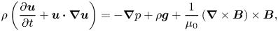 \begin{gather}\rho \left( \frac{\partial \boldsymbol{u}}{\partial t} + \boldsymbol{u}\boldsymbol{\cdot} \boldsymbol{\nabla} \boldsymbol{u} \right) ={-}\boldsymbol{\nabla} p + \rho \boldsymbol{g} + \frac{1}{\mu_0} \left( \boldsymbol{\nabla}\times \boldsymbol{B} \right) \times \boldsymbol{B}, \end{gather}
 \begin{gather}\frac{\partial \boldsymbol{B}}{\partial t} + \left( \boldsymbol{u} \boldsymbol{\cdot} \boldsymbol{\nabla} \right) \boldsymbol{B} = \left( \boldsymbol{B} \boldsymbol{\cdot} \boldsymbol{\nabla} \right) \boldsymbol{u} - \boldsymbol{B} \left( \boldsymbol{\nabla}\boldsymbol{\cdot} \boldsymbol{u} \right), \end{gather}
 \begin{gather}\frac{\partial p}{\partial t} + \boldsymbol{u} \boldsymbol{\cdot} \boldsymbol{\nabla} p + \gamma p \boldsymbol{\nabla}\boldsymbol{\cdot} \boldsymbol{u} = 0, \end{gather}
 \begin{gather}p = \mathcal{R} \rho T, \end{gather}
where  $\mathcal {R} = c_p - c_v$ is the specific gas constant; $c_p$ and $c_v$ are the specific heats at constant pressure and volume, respectively; $\gamma = c_p/c_v$ is the ratio of specific heats; $\mu _0$ is the magnetic permeability of free space; $\boldsymbol{g}$ is the gravitational acceleration. Throughout this paper, the geometry under consideration consists of a plane layer of fluid bounded by horizontal planes located at $z = 0$ and $z = d$, with the $z$-axis pointing downwards ( $\boldsymbol{g} = g \hat {\boldsymbol{e}}_z$). In Cartesian coordinates, we write the fluid velocity as $\boldsymbol{u} = (u,v,w)$. Note that in the above system, which has no dissipation, the dynamics is described completely through (2.1)–(2.4), which involve only the thermodynamic variables $p$ and $\rho$. It is, however, helpful also to introduce the temperature through the perfect gas equation of state (2.5).
The governing equations (2.1)–(2.5) can be written in dimensionless form by scaling magnetic field, mass density, temperature and pressure with their values at the top of the layer ( $z=0$): $B_r$, $\rho _r$, $T_r$ and $p_r = \mathcal {R} \rho _r T_r$, respectively. (The subscript ‘ $r$’ is used throughout to denote representative values of quantities.) Furthermore, we scale lengths with the layer depth $d$, time with the acoustic time scale $d/\sqrt {\mathcal {R} T_r}$ and velocities with $\sqrt {\mathcal {R} T_r}$. Representative values for the square of the isothermal sound speed and the square of the Alfvén speed are, respectively, $c_{s,r}^2 = p_r/\rho _r$, $c_{A,r}^2 = B_r^2/(\mu _0 \rho _r)$. A representative pressure scale height in a hydrostatically balanced atmosphere is $H_r = p_r/(\rho _r g)$. This implies the following relation:
 \begin{equation} c_{s,r}^2 = \frac{p_r}{\rho_r} = \mathcal{R} T_r = g H_r. \end{equation}
The dimensionless equations of compressible MHD then take the form
 \begin{gather} \frac{\partial \rho}{\partial t} + \boldsymbol{\nabla}\boldsymbol{\cdot} \left( \rho \boldsymbol{u} \right) = 0, \end{gather}
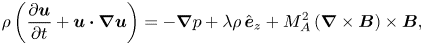 \begin{gather}\rho \left( \frac{\partial \boldsymbol{u}}{\partial t} + \boldsymbol{u}\boldsymbol{\cdot} \boldsymbol{\nabla} \boldsymbol{u} \right) ={-} \boldsymbol{\nabla} p + \lambda \rho \, \hat{\boldsymbol{e}}_z + M_A^2 \left( \boldsymbol{\nabla}\times \boldsymbol{B} \right) \times \boldsymbol{B}, \end{gather}
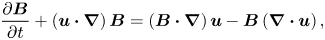 \begin{gather}\frac{\partial \boldsymbol{B}}{\partial t} + \left( \boldsymbol{u} \boldsymbol{\cdot} \boldsymbol{\nabla} \right) \boldsymbol{B} = \left( \boldsymbol{B} \boldsymbol{\cdot} \boldsymbol{\nabla} \right) \boldsymbol{u} - \boldsymbol{B} \left( \boldsymbol{\nabla}\boldsymbol{\cdot} \boldsymbol{u} \right), \end{gather}
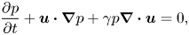 \begin{gather}\frac{\partial p}{\partial t} + \boldsymbol{u} \boldsymbol{\cdot} \boldsymbol{\nabla} p + \gamma p \boldsymbol{\nabla}\boldsymbol{\cdot} \boldsymbol{u} = 0, \end{gather}
 \begin{gather}p = \rho T, \end{gather}
where
 \begin{equation} \lambda = \frac{d}{H_r}, \quad M_A^2 = \frac{B_r^2/\mu_0}{p_r}. \end{equation}
Here,  $\lambda$ is the ratio of the depth of the fluid to the hydrostatic pressure scale height; as such, it is a measure of atmospheric stratification, with small (large) $\lambda$ indicating weak (strong) stratification. The parameter $M_A$ is the Alfvén Mach number – the ratio of Alfvén speed to isothermal sound speed. Note that $M_A^2 = 2/\beta _p$, where $\beta _p$ – the plasma beta – is the ratio of gas pressure to magnetic pressure.
The equations of compressible MHD (2.7)–(2.11) form the most general set of equations describing MHD behaviour in a stratified, electrically conducting, diffusionless, perfect gas, allowing the description of phenomena that occur on a range of distinct time scales. Of particular note is that the equations describe sound waves (or fast magneto-acoustic waves), the time scale for which is often much shorter than that of other waves or instabilities. Furthermore, in scenarios in which the flows are highly subsonic, the high-frequency sound waves often play no dynamically significant role. It is therefore useful to have a system of equations that filter out sound waves and home in on the dynamics evolving on the slower time scale. Such slow-time dynamics is described by the anelastic approximation.
2.2. The anelastic approximation
The anelastic approximation posits an atmosphere that is almost neutrally buoyant – the reference state – and considers the evolution of perturbations on top of that state. Convective instability is governed by the well-known Schwarzschild criterion, which dictates that instability depends on the gradient of specific entropy  $s = c_v \ln (p \rho ^{-\gamma })$: an unstable configuration is one in which specific entropy increases with depth, i.e. $\mathrm {d} s/\mathrm {d} z > 0$. The reference state for the anelastic approximation is thus taken to be one of hydrostatic balance in which entropy is nearly constant (also referred to as near-adiabatic stratification), but with significant variations individually in pressure and density. The small departure from adiabatic stratification induces convection if $\mathrm {d} s/\mathrm {d} z > 0$, or gravity waves if $\mathrm {d} s/\mathrm {d} z < 0$, each of which engenders small perturbations to the reference state.
By treating the departure from adiabatic stratification as a small parameter, one can conduct a formal asymptotic expansion of the compressible equations to extract equations – the anelastic equations – that describe how the perturbations evolve on top of the fixed thermodynamic background. We thus introduce the quantity  $\Delta\!\!\nabla$, a measure of departure from adiabaticity, defined by
 \begin{equation} \Delta\!\!{\nabla} ={-}\frac{d}{H_p} \left( \frac{\mathrm{d} \ln \rho}{\mathrm{d} \ln p} - \left( \frac{\mathrm{d} \ln \rho}{\mathrm{d} \ln p} \right)_{ad} \right), \end{equation}
where
 \begin{equation} H_p = \left( \frac{\mathrm{d} \ln p}{\mathrm{d} z} \right)^{{-}1} \quad \textrm{and} \quad \left( \frac{\mathrm{d} \ln \rho}{\mathrm{d} \ln p} \right)_{ad} = 1/\gamma \end{equation}
are, respectively, the pressure scale height and the adiabatic gradient. The stratification is superadiabatic (convectively unstable) in regions where  $\Delta\!\!\nabla > 0$, and subadiabatic (convectively stable) where $\Delta\!\!\nabla < 0$. The departure from adiabaticity $\Delta\!\!\nabla$ is essentially the dimensionless gradient of specific entropy
 \begin{equation} \frac{\mathrm{d} s}{\mathrm{d} z} \equiv \frac{c_p}{d} \Delta\!\!{\nabla}. \end{equation}
Given that the fundamental requirement of the anelastic approximation is that the atmospheric stratification is close to adiabatic, this allows us to define a small parameter  $\varepsilon$ by
 \begin{equation} \varepsilon = \left| \Delta\!\!{\nabla}_r \right| \ll 1. \end{equation}
Specific entropy is thus constant to the lowest (zeroth) order:  $\mathrm {d} s /\mathrm {d} z = {O}(\varepsilon )$. Since the entropy gradient is the central quantity in the anelastic formulation, it is more convenient to use the entropy formulation of the conservation of internal energy (2.4),
 \begin{equation} \rho T \left( \frac{\partial s}{\partial t} + \boldsymbol{u}\boldsymbol{\cdot} \boldsymbol{\nabla} s \right) = 0.\end{equation}
The assumed small departure from adiabaticity sets the scale for all thermodynamic perturbations, allowing a decomposition of the thermodynamic variables into  $z$-dependent steady reference states, denoted by overbars, and dynamically induced time-dependent fluctuations, denoted by asterisks:
 \begin{equation} \left.\begin{gathered} p = p_r (\bar{p} + \varepsilon p^*),\quad \rho = \rho_r (\bar{\rho} +\varepsilon \rho^*), \\ T = T_r (\bar{T} + \varepsilon T^*),\quad s = s_r + c_p \varepsilon(\bar{s} + s^*), \end{gathered}\right\} \end{equation}
where  $\bar p$, $p^*$, etc. are dimensionless quantities. The scaling for velocity follows from the physical picture that fluid motions arise owing to buoyancy variations; thus, balancing inertia against buoyancy perturbations implies that $u_r^2 \sim \varepsilon g d$. This, in turn, dictates that the time scale is long (slow evolution), with $t \sim d/u_r \sim \varepsilon ^{-1/2} \sqrt {d/g}$. Note that the ordering of velocity means that the flow Mach number (the ratio of flow speed to sound speed) is small, i.e. from (2.6), $M = u_r/c_{s,r} \sim \varepsilon ^{1/2}$, provided that $\lambda$ is ${O}(1)$. In the standard formulation of the anelastic equations, it is assumed that the Lorentz force does not contribute to the hydrostatic balance at lowest order; this implies that the magnetic field must also scale with $\varepsilon$. Balancing the Lorentz force with pressure perturbations yields $B_r^2/\mu _0 \sim \varepsilon p_r$: thus the Alfvén Mach number is small, i.e. $M_A = c_{A,r}/c_{s,r} \sim \varepsilon ^{1/2}$. Based on these considerations, it is useful to introduce scaled parameters, defined by $B_r = \varepsilon ^{1/2} \tilde {B}_r$, $c_{A,r} = \varepsilon ^{1/2} \tilde {c}_{A,r}$, $M_A = \varepsilon ^{1/2} \tilde {M}_A$, where tilde variables and parameters are ${O}(1)$. In terms of the ordering with $\varepsilon$, the natural scalings of length, time, velocity and magnetic field are therefore as follows:
 \begin{equation} \boldsymbol{x}= d \boldsymbol{x}' , \quad t = \varepsilon^{{-}1/2} \left(\frac{d}{c_{s,r}} \right) t^*, \quad \boldsymbol{u} = \varepsilon^{1/2} c_{s,r} \boldsymbol{u}^* , \quad \boldsymbol{B} = \varepsilon^{1/2} \tilde{B}_r \boldsymbol{B}^*, \end{equation}
where, as earlier, we use asterisks to denote (dimensionless) variables that have been scaled with a power of  $\varepsilon$. The formulation proceeds by substituting expressions (2.19a–d) into the compressible MHD equations (2.7)–(2.11) (dropping $'$ superscripts on length variables) and equating terms at successive powers of $\varepsilon$. At ${O}(\varepsilon ^0)$ we obtain non-trivial expressions only from the $z$-component of (2.8) and from (2.11); these define the reference state by
 \begin{gather} \frac{\mathrm{d} \bar{p}}{\mathrm{d} z} =\lambda \bar{\rho} , \end{gather}
 \begin{gather}\bar{p} = \bar{\rho} \bar{T}. \end{gather}
At  ${O}(\varepsilon ^1)$ we obtain the following evolution equations governing the perturbations:
 \begin{gather} \boldsymbol{\nabla}\boldsymbol{\cdot} \left( \bar{\rho} \boldsymbol{u}^* \right) = 0, \end{gather}
 \begin{gather}\bar{\rho} \left( \frac{\partial \boldsymbol{u}^*}{\partial t^*} + \boldsymbol{u}^*\boldsymbol{\cdot} \boldsymbol{\nabla} \boldsymbol{u}^* \right) ={-} \boldsymbol{\nabla} p^* + \lambda \rho^* \hat{\boldsymbol{e}}_z + \tilde{M}_A^2 \left( \boldsymbol{\nabla}\times \boldsymbol{B}^* \right) \times \boldsymbol{B}^*, \end{gather}
 \begin{gather}\frac{\partial \boldsymbol{B}^*}{\partial t^*} + \left( \boldsymbol{u}^* \boldsymbol{\cdot} \boldsymbol{\nabla} \right) \boldsymbol{B}^* = \left( \boldsymbol{B}^* \boldsymbol{\cdot} \boldsymbol{\nabla} \right) \boldsymbol{u}^* - \boldsymbol{B}^* \left( \boldsymbol{\nabla}\boldsymbol{\cdot} \boldsymbol{u}^* \right), \end{gather}
 \begin{gather}\frac{\partial s^*}{\partial t^*} + \boldsymbol{u}^* \boldsymbol{\cdot} \boldsymbol{\nabla} s^* + w^* \frac{\mathrm{d} \bar{s}}{\mathrm{d} z}= 0, \end{gather}
 \begin{gather}\frac{p^*}{\bar{p}} = \frac{\rho^*}{\bar{\rho}} + \frac{T^*}{\bar{T}}, \end{gather}
 \begin{gather}s^* = \frac{T^*}{\bar{T}} - \frac{(\gamma - 1)}{\gamma} \frac{p^*}{\bar{p}}, \end{gather}
where  $\boldsymbol{u}^*=(u^*, v^*, w^*)$. The reference state entropy gradient, of ${O}(\varepsilon )$, is
 \begin{equation} \varepsilon \frac{\mathrm{d} \bar{s}}{\mathrm{d} z} = \frac{1}{\gamma}\frac{\mathrm{d} }{\mathrm{d} z} \left( \ln \bar{p} \bar{\rho}^{-\gamma} \right). \end{equation}
Equations (2.22)–(2.27) constitute the equations of anelastic MHD in dimensionless form.
A further simplification of the anelastic momentum equation may be realised by subsuming the reference state density into the pressure gradient term and also by using (2.26), (2.27) to eliminate the density perturbation in the buoyancy term in favour of  $s^*$ and $p^*$. Thus we obtain
 \begin{equation} -\frac{1}{\bar{\rho}} \boldsymbol{\nabla} p^* + \frac{\lambda \rho^*}{\bar{\rho}} \hat{\boldsymbol{e}}_z ={-} \boldsymbol{\nabla} \left( \frac{p^*}{\bar{\rho}} \right) - \lambda s^* \hat{\boldsymbol{e}}_z - \frac{p^*}{\bar{\rho}} \left[ \frac{1}{\bar{\rho}} \frac{\mathrm{d} \bar{\rho}}{\mathrm{d} z} - \frac{\lambda \bar{\rho} }{\gamma \bar{p}} \right] \hat{\boldsymbol{e}}_z. \end{equation}
For a near-adiabatic reference state,
 \begin{equation} \frac{\mathrm{d} }{\mathrm{d} z} \left( \frac{1}{\gamma}\ln \bar{p}\bar{\rho}^{-\gamma} \right) = \frac{1}{\gamma \bar{p}}\frac{\mathrm{d} \bar{p}}{\mathrm{d} z} - \frac{1}{\bar{\rho}}\frac{\mathrm{d} \bar{\rho}}{\mathrm{d} z} = {O}(\varepsilon) . \end{equation}
On using the equation of hydrostatic balance (2.20), it therefore follows that
 \begin{equation} \frac{1}{\bar{\rho}}\frac{\mathrm{d} \bar{\rho}}{\mathrm{d} z} = \frac{ \lambda \bar{\rho} }{\gamma \bar{p}} + {O}(\varepsilon) . \end{equation}
The term in the square brackets on the right-hand side of (2.29) is thus formally smaller than the other two terms; the momentum equation (2.23) therefore becomes
 \begin{equation} \frac{\partial \boldsymbol{u}^*}{\partial t^*} + \boldsymbol{u}^*\boldsymbol{\cdot} \boldsymbol{\nabla} \boldsymbol{u}^* ={-} \boldsymbol{\nabla} \left( \frac{p^*}{\bar{\rho}} \right) - \lambda s^* \hat{\boldsymbol{e}}_z + \frac{\tilde{M}_A^2 }{\bar{\rho}} \left( \boldsymbol{\nabla}\times \boldsymbol{B}^* \right) \times \boldsymbol{B}^* . \end{equation}
This simplification of the momentum equation was demonstrated by Lantz (Reference Lantz1992) and Braginsky & Roberts (Reference Braginsky and Roberts1995). It is important to note that it requires no additional approximation, but follows immediately from the original assumption of a near-adiabatic reference state; i.e. (2.23) and (2.32) are asymptotically equivalent leading-order expressions.
In the course of the following analysis it will sometimes be advantageous to work with the governing equations in their dimensional form, which we therefore state here for completeness. Equations (2.22), (2.24), (2.25) and (2.26) are unchanged. In dimensional form, the two versions of the momentum equation (2.23) and (2.32), and the thermodynamic relation (2.27) read as
 \begin{gather} \bar{\rho} \left( \frac{\partial \boldsymbol{u}^*}{\partial t^*} + \boldsymbol{u}^*\boldsymbol{\cdot} \boldsymbol{\nabla} \boldsymbol{u}^* \right) ={-} \boldsymbol{\nabla} p^* + \rho^* g \hat{\boldsymbol{e}}_z + \frac{1}{\mu_0} \left( \boldsymbol{\nabla}\times \boldsymbol{B}^* \right) \times \boldsymbol{B}^*, \end{gather}
 \begin{gather}\frac{\partial \boldsymbol{u}^*}{\partial t^*} + \boldsymbol{u}^*\boldsymbol{\cdot} \boldsymbol{\nabla} \boldsymbol{u}^* ={-} \boldsymbol{\nabla} \left( \frac{p^*}{\bar{\rho}} \right) - \frac{s^*}{c_p} g \hat{\boldsymbol{e}}_z + \frac{1}{\mu_0 \bar{\rho}} \left( \boldsymbol{\nabla}\times \boldsymbol{B}^* \right) \times \boldsymbol{B}^* . \end{gather}
 \begin{gather}s^* = c_p \frac{T^*}{\bar{T}} - (c_p - c_v) \frac{p^*}{\bar{p}} . \end{gather}
The dimensional equations governing the reference state are
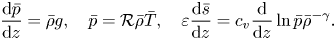 \begin{equation} \frac{\mathrm{d} \bar{p}}{\mathrm{d} z} = \bar{\rho}g, \quad \bar{p} = \mathcal{R} \bar{\rho} \bar{T},\quad \varepsilon \frac{\mathrm{d} \bar{s}}{\mathrm{d} z} = c_v \frac{\mathrm{d} }{\mathrm{d} z} \ln{\bar{p} \bar{\rho}^{-\gamma}}. \end{equation}
2.3. The subtle ordering for magnetic buoyancy
As can be seen from the formulation above, the magnetic field is incorporated into the anelastic approximation in a straightforward way, with the only requirement being that the field is sufficiently weak. On the other hand, including the effects of magnetic buoyancy in the Boussinesq approximation is a subtle procedure, which, inter alia, involves consideration of the length scale characteristic of magnetic buoyancy perturbations (Spiegel & Weiss Reference Spiegel and Weiss1982; Corfield Reference Corfield1984; Bowker et al. Reference Bowker, Hughes and Kersalé2014). Specifically, the requirement that the length scale of motions in the direction of the imposed horizontal magnetic field be long in comparison with the transverse scale has to be built into the approximation. In the anelastic system, however, no such special measures are taken to ensure that magnetic buoyancy is included consistently. The question thus arises as to whether the anelastic equations do indeed retain the effects of magnetic buoyancy, and, if so, why are no special measures required governing the length scale of the perturbation? Here, we seek to elucidate this matter by examining the fundamental ordering of the physical quantities necessary for magnetic buoyancy instability, thus clarifying the relationship between the descriptions of magnetic buoyancy in the full (compressible) and reduced (anelastic, Boussinesq) systems. By striking the appropriate balances between terms in the governing equations, we derive the general scalings necessary to account for the effects of magnetic buoyancy in the reduced equations. The resulting scalings allow us to identify, and distinguish between, different reduced systems (or regimes) of the full compressible MHD equations.
As above, we consider an atmosphere of depth  $d$ and pressure scale height $H_p = p_r/(\rho _r g)$. In the basic state, we assume an imposed horizontal magnetic field, stratified in the vertical direction with scale height $H_B$. When the system is perturbed, and motions ensue, the presence of the imposed horizontal field introduces a length scale in the direction of the field that may be distinct from both $d$ and $H_B$: we denote this length scale by $L_B$. For any variable $f$, we define $f_r$ and $\delta f$ to be, respectively, representative values of $f$ in equilibrium and of the magnitude of fluctuations of $f$. For vector fields, it is necessary to distinguish between components aligned with, and those perpendicular to, the imposed magnetic field. We denote the magnitudes of the components of the fluctuations parallel and perpendicular to the imposed field by subscripts $\parallel$ and $\perp$, respectively.
By considering the magnitudes of the fluctuating quantities in the dimensional compressible equations (2.1)–(2.5), we will establish the relation that must be obeyed between the various length scales of the problem if magnetic buoyancy is to be of significance. We will pursue, in a slightly more general fashion, the line of argument expounded by Bowker et al. (Reference Bowker, Hughes and Kersalé2014). First, from the momentum equation (2.2), balancing the inertia term with those of total pressure fluctuations, buoyancy and magnetic tension gives
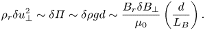 \begin{equation} \rho_r \delta u_\perp^2 \sim \delta \varPi \sim \delta\rho g d \sim \frac{B_r \delta B_\perp}{\mu_0} \left( \frac{d}{L_B} \right) . \end{equation}
With our focus on buoyancy-driven instabilities, the time scale is determined by the balance of vertical acceleration and buoyancy, thus giving the scaling
 \begin{equation} \frac{\partial }{\partial t}\sim \frac{\delta u_\perp}{d}. \end{equation}
From the balance between inertia and buoyancy in (2.37), we may express the kinetic energy of the transverse flow in terms of the density variation as
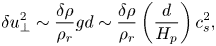 \begin{equation} \delta u_\perp^2 \sim \frac{\delta \rho}{\rho_r} gd \sim \frac{\delta \rho}{\rho_r} \left( \frac{d}{H_p} \right) c_s^2, \end{equation}
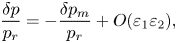
where  $c_s^2 = p_r/\rho _r$. The scaling for total pressure fluctuations, $\delta \varPi = \delta p + \delta p_m$, results from balancing the gradient of total pressure fluctuations with the inertia terms, and hence with the buoyancy, thus,
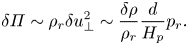 \begin{equation} \delta \varPi \sim \rho_r \delta u_\perp^2 \sim \frac{\delta \rho}{\rho_r} \frac{d}{H_p} p_r. \end{equation}
Balancing advection and stretching terms in the parallel and perpendicular components of the induction equation (2.3) results in the following relations:
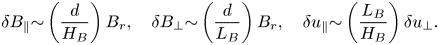 \begin{equation} \delta B_\parallel{\sim} \left( \frac{d}{H_B} \right) B_r, \quad \delta B_\perp{\sim} \left( \frac{d}{L_B} \right) B_r, \quad \delta u_\parallel{\sim} \left( \frac{L_B}{H_B} \right) \delta u_\perp . \end{equation}
From the balance between buoyancy and magnetic tension in (2.37), together with (2.41b), the density variation may be expressed in terms of the representative field strength as
 \begin{equation} \frac{\delta \rho}{\rho_r} \sim \left(\frac{B_r^2}{\mu_0 p_r} \right) \left( \frac{H_p}{d} \right) \left( \frac{d}{L_B} \right)^2 . \end{equation}
It should be noted that (2.42) expresses the contribution to the density variation arising from the magnetic field, which is of particular interest here. There will of course also be a contribution arising from entropy variations, which is present even in the absence of field. From (2.41a) and (2.42), the magnetic pressure variation may be expressed as
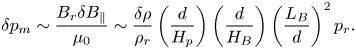 \begin{equation} \delta p_m \sim \frac{B_r \delta B_\parallel}{\mu_0} \sim \frac{\delta \rho}{\rho_r} \left( \frac{d}{H_p} \right) \left( \frac{d}{H_B} \right) \left( \frac{L_B}{d} \right)^2 p_r. \end{equation}
The above orderings are quite general, insofar as they arise simply from balancing terms in the governing equations, but with no assumptions having been made about the magnitude of the density fluctuation  $\delta \rho$ relative to the background $\rho _r$, nor of the relative magnitudes of the length scales $d$,
$d$,  $H_p$, $H_B$ and $L_B$.
Note that both the anelastic and Boussinesq approximations assume that the size of thermodynamic fluctuations is small compared with their background values:  ${\delta \rho /\rho _r \ll 1}$. The anelastic approximation is valid for stratified atmospheres whose vertical extent can span many pressure scale heights: $d \geqslant H_p$. The Boussinesq approximation is more restrictive as it applies only to weakly stratified atmospheres – ones whose depth is much smaller than the pressure scale height: $d \ll H_p$.
For magnetic pressure fluctuations to be influential – a necessary condition for magnetic buoyancy instability – they must be comparable in magnitude to density fluctuations:  $\delta p_m / p_r \sim \delta \rho /\rho _r$. From (2.43), we deduce that this requirement imposes the following important relation between length scales:
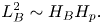 \begin{equation} L_B^2 \sim H_B H_p . \end{equation}
To establish the consistency of the above argument, it is instructive to substitute for  $L_B^2$ from (2.44) into (2.42), which gives the density variation due to the magnetic field as
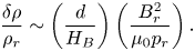 \begin{equation} \frac{\delta \rho}{\rho_r} \sim \left( \frac{d}{H_B}\right) \left(\frac{B_r^2}{\mu_0 p_r} \right) . \end{equation}
Thus, for a fixed  $H_B$, the field will not influence the density if $B_r$ is sufficiently weak; conversely, the influence of the field is accentuated by very small values of $H_B$.
From the relation (2.44), we are able to identify four distinct regimes in which magnetic buoyancy is faithfully described – two in the anelastic approximation and two in the Boussinesq approximation – together with a further Boussinesq regime in which the effects of magnetic buoyancy are explicitly excluded. These distinct regimes, or reduced systems, are explained in more detail in the following subsection. Furthermore, each reduced system has its own distinctive set of governing equations, which are provided in the Appendix.
2.4. Distinguished regimes of the anelastic and Boussinesq approximations
In order to categorise the five possible regimes, we define the following ordering parameters:
 \begin{equation} \varepsilon_1 = \frac{d}{H_p}, \quad \varepsilon_2 = \frac{\delta \rho}{\rho_r}, \quad \varepsilon_B = \frac{d}{H_B}. \end{equation}
The definitions of  $\varepsilon _1$ and $\varepsilon _2$ are in accordance with the notation used in Corfield (Reference Corfield1984) and Bowker et al. (Reference Bowker, Hughes and Kersalé2014). Note also that $\varepsilon _2$ is equivalent to the parameter $\varepsilon$ used to derive the anelastic equations in § 2.2. For all the various approximations, thermodynamic fluctuations are considered small: $\varepsilon _2 \ll 1$.
It is important to consider how the entropy gradient comes into this ordering. The background entropy gradient must be of the size of thermodynamic fluctuations (at most); otherwise, the assumption that  $\delta \rho /\rho _r \ll 1$ would not be justified. Indeed, this is an explicit requirement of the anelastic approximation. Likewise, the same ordering of the entropy gradient ( $\mathrm {d} s/\mathrm {d}z \sim \varepsilon _2$) pertains to the Boussinesq approximation (Spiegel & Weiss Reference Spiegel and Weiss1982).
2.4.1. Standard anelastic approximation
The derivation of the anelastic equations in § 2.2 involved no special consideration of the magnetic scale height  $H_B$, de facto treating it as on a par with the layer depth: ${d \sim H_B}$. Likewise, making no distinction between the parallel and perpendicular directions amounts to an implicit assumption that $L_B \sim d$. With $d/H_p = {O}(1)$, it follows that all the length scales stand on an equal footing, i.e.
 \begin{equation} d \sim H_p \sim H_B \sim L_B. \end{equation}
Crucially, such an ordering satisfies (2.44), the essential length scale relation for magnetic buoyancy. Thus, possibly fortuitously, no special measures need to be taken to incorporate magnetic buoyancy into the standard anelastic approximation. Total pressure variations (2.40) and magnetic pressure variations (2.43) are of the same order of magnitude, with
 \begin{equation} \frac{\delta \varPi}{p_r} \sim \frac{\delta p_m}{p_r} = {O}(\varepsilon_2). \end{equation}
With the ordering of length scales (2.47), the relation (2.42) requires that the magnetic field strength, expressed through the parameter  $M_A^2 = B_r^2/\mu _0 p_r$, is ${O}(\varepsilon _2)$.
2.4.2. Weak field-gradient anelastic approximation
For the case of weak magnetic stratification, i.e.  $H_B \gg d$, it turns out that there is another possible regime within the anelastic framework. In this case, the parallel length scale $L_B$ is necessarily larger than $d$ in order to satisfy the crucial relation for magnetic buoyancy (2.44). More precisely,
 \begin{equation} d \sim H_p, \quad d \ll H_B, \quad L_B \sim \sqrt{ d H_B}. \end{equation}
As for the ordering (2.47), variations in total and magnetic pressure obey (2.48). However, with a weak field gradient ( $H_B \gg d$), the magnetic field needs to be stronger than in § 2.4.1 in order to compensate for the weak gradient; thus here, again using (2.42), $M_A^2 = {O}(\varepsilon _2/\varepsilon _B)$, with the requirement that $\varepsilon _2/\varepsilon _B \ll 1$, so that the Alfvén speed remains much slower that the sound speed.
2.4.3. Standard magneto-Boussinesq approximation
The length scales in the standard magneto-Boussinesq equations of Spiegel & Weiss (Reference Spiegel and Weiss1982) obey the ordering
 \begin{equation} d \ll H_p, \quad H_B \sim L_B \sim H_p. \end{equation}
The magnitudes of total and magnetic pressure fluctuations are given by
 \begin{equation} \frac{\delta \varPi}{p_r} = {O}(\varepsilon_1 \varepsilon_2), \quad \frac{\delta p_m}{p_r} = {O}(\varepsilon_2). \end{equation}
Thus,
 \begin{equation} \frac{\delta p}{p_r} ={-} \frac{\delta p_m}{p_r} + {O}(\varepsilon_1 \varepsilon_2), \end{equation}
thereby guaranteeing that magnetic pressure variations enter the equation of state to produce density variations. The field strength is given by  $M_A^2 = {O}(\varepsilon _2/\varepsilon _1)$, subject to $\varepsilon _2 \ll \varepsilon _1$, so that the Alfvén speed is much smaller than the sound speed.
2.4.4. Strong field-gradient magneto-Boussinesq approximation
The magneto-Boussinesq orderings, which lead to (2.51a,b) and (2.52), can also be obeyed if the field gradient is much stronger than the pressure gradient (Bowker et al. Reference Bowker, Hughes and Kersalé2014). The precise ordering required is
 \begin{equation} d \ll H_p, \quad H_B \sim d, \quad L_B \sim \sqrt{d H_p}. \end{equation}
Here, the field is weaker than in § 2.4.3, with  $M_A^2 = {O}(\varepsilon _2)$.
2.4.5. Boussinesq magnetoconvection
Under the Boussinesq orderings, it is also possible to include the effects of magnetic tension, but neglect the dynamical influence of magnetic pressure. This gives the well-studied system of Boussinesq magnetoconvection (e.g. Weiss & Proctor Reference Weiss and Proctor2014), in which the length scales obey the following ordering:
 \begin{equation} d \ll H_p, \quad L_B \sim d, \quad H_B \gtrsim d. \end{equation}
As expected, the necessary scaling for the inclusion of magnetic buoyancy, (2.44), is not now satisfied. The key feature of the Boussinesq magnetoconvection ordering is that the variations of both total and magnetic pressure are smaller than density variations ( ${\delta \rho /\rho _r = {O}(\varepsilon _2)}$), with
 \begin{equation} \frac{\delta \varPi}{p_r} \sim \frac{\delta p_m}{p_r} = {O}(\varepsilon_1 \varepsilon_2). \end{equation}
It thus follows that thermodynamic pressure fluctuations  $\delta p/p_r$ are, at most, ${O}(\varepsilon _1 \varepsilon _2)$; hence, to leading order, density variations arise on account only of temperature variations. In this regime the magnetic field is also very weak, with $M_A^2 = {O} (\varepsilon _1 \varepsilon _2)$.
2.4.6. Summarising the five systems
We have described how, within each of the anelastic and magneto-Boussinesq approximations, there are two distinct orderings of the length scales of the problem that allow for the consistent inclusion of the effects of magnetic buoyancy. In addition to that of the standard anelastic system, there is a further distinct ordering with a weaker field gradient, a stronger field and a longer characteristic length scale of the perturbations. Similarly, in addition to the standard magneto-Boussinesq system, there is a distinct ordering with a stronger field gradient, a weaker field and a shorter characteristic length scale of the perturbations. Within the Boussinesq approximation, there is also the ordering that leads to the system of Boussinesq magnetoconvection, in which magnetic buoyancy is excluded.
It is important to note also that the relative magnitudes of  $d$,
$d$,  $H_B$ and $L_B$ determine the relative sizes of the perpendicular and parallel components of the velocity and magnetic fluctuations. Naturally, the ordering of length scales also has implications for the scalings of spatial derivatives parallel and perpendicular to the field:
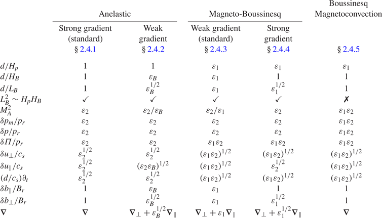
  $\boldsymbol{\nabla } = \boldsymbol{\nabla }_\perp + (d/L_B) \boldsymbol{\nabla }_\parallel$. The scalings of all quantities for each regime are summarised in table 1. On applying the orderings in table 1 to the governing compressible equations, we obtain five distinct reduced systems; these are described in detail in the Appendix. As a final point, we should note why there are three reductions possible under the Boussinesq approximation, but only two under the anelastic approximation. Within the assumptions of the Boussinesq approximation, it is possible to obtain an asymptotically consistent set of equations that includes the effects of magnetic tension but not of magnetic buoyancy – namely, the equations of Boussinesq magnetoconvection. However, within the anelastic approximation, such a reduction is not possible; the influence of the magnetic field is felt both via tension and buoyancy.
Table 1. Summary of orderings in different regimes.
3. Formulation of the linear problem
The upshot of the analysis in the preceding section is that we expect magnetic buoyancy to be well represented by the anelastic equations within the described regime of validity (i.e. with a near-adiabatic stratification and a weak magnetic field). Now, we will put those ideas to the test, quantitatively, by comparing the solutions of the linearised compressible and (standard) anelastic systems. In this section, we formulate the linear eigenvalue problems, for both the compressible and the anelastic systems, which we will solve in §§ 4 and 5. In these later sections, we will actually make use of the linearised equations in both their dimensional and dimensionless forms; since the underlying form of the equations is, of course, the same for both, we will here describe just the dimensionless formulation. We restrict our attention to cases in which the atmospheric stratification is sub-adiabatic, so that the fluid layer is stable to convection and thus magnetic buoyancy is the only destabilising agent. The equilibrium magnetic field is a function of depth and aligned with the  $y$-direction: $B(z) \hat {\boldsymbol{e}}_y$.
3.1. Compressible MHD
In the absence of fluid motion, the (dimensionless) compressible equations admit a steady  $z$-dependent basic-state solution. The basic-state variables (denoted by subscript ‘ $b$’) satisfy the well-known relations for a magnetohydrostatic perfect gas,
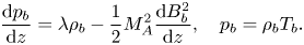 \begin{equation} \frac{\mathrm{d} p_b}{\mathrm{d} z} = \lambda \rho_b - \frac{1}{2} M_A^2 \frac{\mathrm{d} B_b^2}{\mathrm{d} z}, \quad p_b= \rho_b T_b . \end{equation}
Elimination of  $p_b$ between the two equations in (3.1a,b) results in the ordinary differential equation (ODE) for $\rho _b$,
 \begin{equation} \frac{\mathrm{d} \rho_b}{\mathrm{d} z} + \rho_b \varGamma (z) ={-} \frac{1}{2} M_A^2 \frac{1}{T_b} \frac{\mathrm{d} B_b^2}{\mathrm{d} z}, \quad \text{where} \ \varGamma (z) = \frac{\mathrm{d} \ln T_b}{\mathrm{d} z} - \frac{\lambda}{T_b}. \end{equation}
On applying the boundary condition  $\rho _b(z=0) = 1$, (3.2) can be integrated to give
 \begin{equation} \rho_b(z) = \exp \left[ -\int _0^z \varGamma (z) \, \mathrm{d} z \right] \left\lbrace 1 - \frac{1}{2} M_A^2 \int _0^z \frac{1}{T_b} \frac{\mathrm{d} B_b^2}{\mathrm{d} z} \exp \left[ \int _0^z \varGamma (z) \, \mathrm{d} z \right] \, \mathrm{d} z \right\rbrace. \end{equation}
 We consider perturbations to the basic state, expressing velocity, magnetic field and thermodynamic variables in the perturbed state as  $\boldsymbol{\delta u}$, $\boldsymbol{B}_b + \boldsymbol{\delta b}$, $p_b + \delta p$, etc., respectively. On assuming that the perturbations are small, and hence that nonlinear terms may be neglected, we can express all disturbances in the following form:
 \begin{equation} \delta p = \hat{p}(z) \exp({\rm i} \omega t + {\rm i}k_x x +{\rm i} k_y y), \quad \text{etc.}, \end{equation}
where  $\omega$ is the (complex) oscillation frequency and $k_x$ and $k_y$ are the wavenumbers in the $x$ and $y$ horizontal directions. Substituting into the governing equations (2.1)–(2.4) and retaining only the lowest-order terms in the perturbations leads to the following linear system for the perturbations:
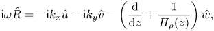 \begin{gather} {\rm i} \omega \hat{R} ={-} {\rm i}k_x \hat{u} - {\rm i}k_y \hat{v} - \left( \frac{\mathrm{d} }{\mathrm{d} z} + \frac{1}{H_\rho(z)} \right) \hat{w} , \end{gather}
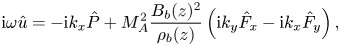 \begin{gather}{\rm i} \omega \hat{u} ={-} {\rm i}k_x \hat{P} + M_A^2 \frac{B_b(z)^2}{\rho_b(z)} \left( {\rm i}k_y \hat{F}_x - {\rm i}k_x \hat{F}_y \right) , \end{gather}
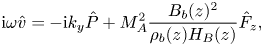 \begin{gather}{\rm i} \omega \hat{v} ={-} {\rm i}k_y \hat{P} + M_A^2 \frac{B_b(z)^2}{\rho_b(z) H_B(z)} \hat{F}_z , \end{gather}
 \begin{gather}{\rm i} \omega \hat{w} ={-} \left( \frac{\mathrm{d} }{\mathrm{d} z} +\frac{1}{H_\rho(z)} \right)\hat{P} + \lambda \hat{R} + M_A^2 \frac{B_b(z)^2}{\rho_b(z)} \left\lbrace- \left( \frac{\mathrm{d} }{\mathrm{d} z} + \frac{2}{H_B(z)} \right) \hat{F}_y + {\rm i} k_y \hat{F}_z \right\rbrace , \end{gather}
 \begin{gather}{\rm i}\omega \hat{F}_x = {\rm i} k_y \hat{u} , \end{gather}
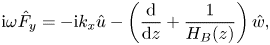 \begin{gather}{\rm i}\omega \hat{F}_y ={-} {\rm i}k_x \hat{u} - \left( \frac{\mathrm{d} }{\mathrm{d} z} + \frac{1}{H_B(z)} \right) \hat{w} , \end{gather}
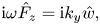 \begin{gather}{\rm i}\omega \hat{F}_z = {\rm i}k_y \hat{w} , \end{gather}
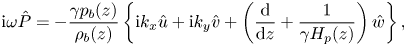 \begin{gather}{\rm i} \omega \hat{P} ={-} \frac{\gamma p_b(z)}{\rho_b(z)}\left\lbrace {\rm i}k_x \hat{u} + {\rm i}k_y \hat{v} + \left( \frac{\mathrm{d} }{\mathrm{d} z} + \frac{1}{\gamma H_p(z)} \right) \hat{w} \right\rbrace , \end{gather}
where  $\hat {R} = \hat {\rho }/\rho _b$, $\hat {P} = \hat {p}/\rho _b$, $\hat {F}_x = \hat {b}_x/B_b$, $\hat {F}_y = \hat {b}_y/B_b$, $\hat {F}_z = \hat {b}_z/B_b$ and
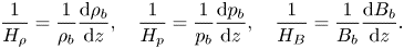 \begin{equation} \frac{1}{H_\rho} = \frac{1}{\rho_b} \frac{\mathrm{d} \rho_b}{\mathrm{d} z}, \quad \frac{1}{H_p} = \frac{1}{p_b} \frac{\mathrm{d} p_b}{\mathrm{d} z}, \quad \frac{1}{H_B} = \frac{1}{B_b} \frac{\mathrm{d} B_b}{\mathrm{d} z}. \end{equation}
Equations (3.5)–(3.12), together with the boundary conditions  $\hat {w} = 0$ at $z = 0, 1$, constitute an eigenvalue problem for the frequency $\omega$. In general, this set of equations requires a numerical solution, which we obtain using Chebyshev differentiation matrices (Trefethen Reference Trefethen2000).
3.2. Anelastic MHD
In the absence of motion, the (dimensional) anelastic equations admit a steady  $z$-dependent basic-state solution (denoted by index ‘0’), which satisfies
 \begin{gather} \frac{\mathrm{d} }{\mathrm{d} z} \left( p_0 + \frac{\tilde{M}_A^2}{2} B_0^2 \right) = \lambda \rho_0 , \end{gather}
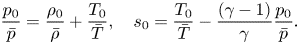 \begin{gather} \frac{p_0}{\bar{p}} = \frac{\rho_0}{\bar{\rho}} + \frac{T_0}{\bar{T}} , \quad s_0 = \frac{T_0}{\bar{T}} - \frac{(\gamma-1)}{\gamma} \frac{p_0}{\bar{p}} . \end{gather}
Note that, since we are considering an ideal system with no diffusivity, we have three equations for the four variables  $\rho _0$, $p_0$, $T_0$, $s_0$. If the thermal and magnetic diffusivity were non-zero, the balance between thermal diffusion and Ohmic heating in the energy equation would provide a relation between $T_0$ and $B_0$. In the ideal case, however, we have the freedom to set $T_0 = 0$. In other words, the imposed field $B_0$ influences the density and pressure stratification (through (3.14)), but does not affect the (steady state) temperature distribution. The basic-state entropy gradient can thus be expressed solely in terms of $\bar {p}$ and $B_0$ as
 \begin{equation} \frac{\mathrm{d} s_0}{\mathrm{d} z} = \frac{(\gamma-1)}{\gamma} \tilde{M}_A^2 \frac{B_0}{\bar{p}} \frac{\mathrm{d} B_0}{\mathrm{d} z}. \end{equation}
 We express velocity, magnetic field and thermodynamic variables in the perturbed state as  $\boldsymbol{\delta u}^*$, $\boldsymbol{B}_0 + \boldsymbol{\delta b}^*$, $s_0 + \delta s^*$, etc., respectively. As for the full compressible equations, we now consider small perturbations to the basic state, allowing us to express all disturbances as
 \begin{equation} \delta s^* = \hat{s}^*(z) \exp({\rm i} \tilde{\omega} t + {\rm i}k_x x +{\rm i}k_y y), \quad \text{etc.}, \end{equation}
where the tilde notation on the eigenvalue reflects the different time scaling between the compressible and anelastic systems (cf. (3.4))). Substituting expressions (3.17) into the governing equations (2.22), (2.32), (2.24), (2.25), and retaining only the lowest-order terms in the perturbations, leads to the following set of (dimensionless) perturbation equations:
 \begin{gather} 0={\rm i} k_x \hat{u}^* + {\rm i} k_y \hat{v}^* + \left( \frac{\mathrm{d} }{\mathrm{d} z} + \frac{1}{ \bar{H}_\rho(z)} \right) \hat{w}^* , \end{gather}
 \begin{gather}{\rm i} \tilde{\omega} \hat{u}^* ={-} {\rm i} k_x \hat{P}^* + \tilde{M}_A^2 \frac{B_0(z)^2}{\bar{\rho}(z)} \left( {\rm i} k_y \hat{F}_x^* - {\rm i} k_x \hat{F}_y^* \right) , \end{gather}
 \begin{gather}{\rm i} \tilde{\omega} \hat{v}^* ={-} {\rm i} k_y \hat{P}^* + \tilde{M}_A^2 \frac{B_0(z)^2}{\bar{\rho}(z) H_B(z)} \hat{F}_z^* , \end{gather}
 \begin{gather}{\rm i} \tilde{\omega} \hat{w}^* ={-} \frac{\mathrm{d} \hat{P}^*}{\mathrm{d} z} - \lambda \hat{s}^* +\tilde{M}_A^2 \frac{B_0(z)^2}{\bar{\rho}(z)}\left\lbrace - \left( \frac{\mathrm{d} }{\mathrm{d} z} +\frac{2}{H_B(z)} \right) \hat{F}_y^* + {\rm i} k_y \hat{F}_z^* \right\rbrace , \end{gather}
 \begin{gather}{\rm i} \tilde{\omega} \hat{F}_x^* = {\rm i} k_y \hat{u}^* , \end{gather}
 \begin{gather}{\rm i} \tilde{\omega} \hat{F}_y^* = {\rm i} k_y \hat{v}^* + \left( \frac{1}{\bar{H}_\rho(z)} - \frac{1}{H_B(z)} \right) \hat{w}^* , \end{gather}
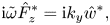 \begin{gather}{\rm i} \tilde{\omega} \hat{F}_z^* = {\rm i} k_y \hat{w}^* , \end{gather}
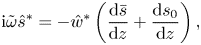 \begin{gather}{\rm i} \tilde{\omega} \hat{s}^* ={-} \hat{w}^* \left( \frac{\mathrm{d} \bar{s}}{\mathrm{d} z} + \frac{\mathrm{d} s_0}{\mathrm{d} z} \right) , \end{gather}
where  $\hat {P}^* =\hat {p}^*/\bar {\rho }$, $\hat {F}_x^* = \hat {b}_x^*/B_0$, $\hat {F}_y^* = \hat {b}_y^*/B_0$, $\hat {F}_z^* = \hat {b}^*_z/B_0$ and
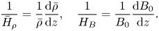 \begin{equation} \frac{1}{\bar{H}_\rho} = \frac{1}{\bar{\rho}} \frac{\mathrm{d} \bar{\rho}}{\mathrm{d} z}, \quad \frac{1}{H_B} = \frac{1}{B_0} \frac{\mathrm{d} B_0}{\mathrm{d} z} . \end{equation}
As for the compressible system, the general solution of the eigenvalue problem defined by (3.18)–(3.25) requires numerical treatment.
3.3. Comparing solutions to the compressible and anelastic systems
Before proceeding to the analysis of the solutions of the compressible and anelastic systems, it is important to explain the relations between the parameters and variables pertaining to the two systems. The two systems differ in terms of time and velocity scales; by design, the anelastic system governs the dynamics of slow motions evolving on a long time scale. Thus, comparing the velocities and eigenvalues of the compressible system with those of the anelastic system requires the following scaling:  $| \boldsymbol{u}| = \varepsilon ^{1/2} |\boldsymbol{u}^*|$, $\omega = \varepsilon ^{1/2} \tilde {\omega }$. Since we have used the same scaling for the magnetic field ( $B_r$) for the two systems, no re-scaling is needed when comparing magnetic field perturbations. Note, however, that $M_A^2= \varepsilon \tilde {M}_A^2$.
In the compressible system, the basic-state density and pressure correspond to the sum of the reference and basic states of the anelastic system; thus,  $\rho _b = \bar {\rho } + \varepsilon \rho _0$ and $p_b = \bar {p} + \varepsilon p_0$. For the temperature, however, $T_b = \bar {T}$ since, in ideal MHD, we have the freedom to impose one of the equilibrium thermodynamic quantities. An important difference between the two systems is that, in the anelastic case, the background reference state is strictly adiabatic (i.e. the static solution profiles $\bar {\rho }$, $\bar {p}$, $\bar {T}$ are such that the departure from adiabaticity $\Delta\!\!\nabla$ is strictly zero); the asymptotically small entropy gradient enters only into the prognostic equations, but not the background state. The basic state entropy gradient in the compressible system is given by
 \begin{equation} \frac{\mathrm{d} s_b}{\mathrm{d} z} = \frac{\mathrm{d} }{\mathrm{d} z} \left( \frac{1}{\gamma} \ln \left( \frac{p_b}{\rho_b^{\gamma}} \right) \right) = \left( \frac{\mathrm{d} T_b}{\mathrm{d} z} - \frac{\left( \gamma - 1 \right)}{\gamma} \lambda \right) \frac{1}{T_b} + \frac{\left( \gamma - 1 \right)}{\gamma} M_A^2 \left( \frac{B_b}{p_b} \right) \frac{\mathrm{d} B_b}{\mathrm{d} z}; \end{equation}
this is related to the reference and basic-state entropy gradients of the anelastic system as follows:
 \begin{equation} \frac{\mathrm{d} s_b}{\mathrm{d} z} = \varepsilon \frac{\mathrm{d} \bar{s}}{\mathrm{d} z} + \varepsilon \frac{\mathrm{d} s_0}{\mathrm{d} z} + {O}(\varepsilon^2). \end{equation}
4. Instabilities of a constant Alfvén speed atmosphere
As noted above, the linear eigenvalue problem resulting from a small perturbation of a magnetohydrostatic atmosphere typically requires a numerical solution – for both the compressible and anelastic systems. However, for the special case where the basic-state atmosphere is isothermal with a constant Alfvén speed, the perturbation equations possess a simple analytical solution, allowing the dispersion relation to be written explicitly. This is extremely illuminating, since it allows a rigorous comparison between the two systems. For the compressible MHD equations, the dispersion relation was derived by Yu (Reference Yu1965) and Chen & Lykoudis (Reference Chen and Lykoudis1972); we will derive presently the dispersion relation for the anelastic system.
It is illustrative to begin with the dimensional equations since the various speeds that arise then appear explicitly in the dispersion relations. However, the ensuing comparison between the two systems will require suitable rescaling.
4.1. Compressible case
The equilibrium state is given by
 \begin{equation} \rho_b = \rho_r \exp\left( \frac{z}{H} \right), \quad p_b = p_r \exp\left( \frac{z}{H} \right), \quad T_b = T_r, \quad B_b = B_r \exp\left( \frac{z}{2H} \right), \end{equation}
where the (magnetohydrostatic) scale height  $H$ satisfies
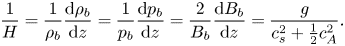 \begin{equation} \frac{1}{H} = \frac{1}{\rho_b} \frac{\mathrm{d} \rho_b}{\mathrm{d} z} = \frac{1}{p_b} \frac{\mathrm{d} p_b}{\mathrm{d} z} = \frac{2}{B_b} \frac{\mathrm{d} B_b}{\mathrm{d} z} = \frac{g}{c_s^2 + \frac{1}{2} c_A^2} . \end{equation}
The linearised equations of compressible MHD (the dimensional versions of (3.5)–(3.11)) can be combined to give the following single second-order ODE for  $\hat {w}$:
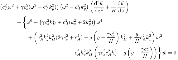 \begin{align} &\left( c_A^2 \omega^2 + \gamma c_s^2(\omega^2 - c_A^2 k_y^2) \right) \left( \omega^2 - c_A^2 k_y^2 \right) \left( \frac{\mathrm{d}^2 \hat{w}}{\mathrm{d} z ^2} + \frac{1}{H} \frac{\mathrm{d} \hat{w}}{\mathrm{d} z} \right)\nonumber\\ &\hskip1.8pc\quad + \left\lbrace \vphantom{\left( \gamma c_s^2 c_A^2 k_y^2 - g\left( g-\frac{\gamma c_s^2}{H} \right) \right)}\omega^6 - \left( \gamma c_s^2 k_H^2 + c_A^2 (k_x^2 +2k_y^2) \right) \omega^4 \right. \nonumber\\ &\hskip3.5pc\quad + \left( c_A^2 k_y^2 k_H^2 (2\gamma c_s^2 +c_A^2) -g\left( g - \frac{\gamma c_s^2}{H} \right)k_H^2 + \frac{g}{H}c_A^2 k_x^2 \right) \omega^2 \nonumber\\ &\hskip10pc\quad \left.- c_A^2 k_y^2 k_H^2 \left( \gamma c_s^2 c_A^2 k_y^2 - g\left( g-\frac{\gamma c_s^2}{H} \right) \right) \right\rbrace \hat{w} = 0, \end{align}
where  $k_H^2 = k_x^2 + k_y^2$. Subject to the impermeable boundary conditions $\hat {w} = 0$ on $z = 0$ and $z=d$, the ODE (4.3) admits a solution $\hat {w} \propto \exp \left ( -z/2H \right ) \sin \left ( k_z z \right )$, with $k_z = n {\rm \pi}/d$ (where mode $n = 1$ is the most readily destabilised). Substituting the ansatz for $\hat w$ into (4.3) yields the dispersion relation
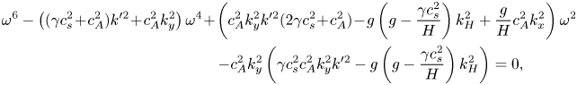 \begin{gather} \omega^6 - \left( (\gamma c_s^2 \!+\! c_A^2)k'^2 \!+\! c_A^2 k_y^2 \right) \omega^4 \!+\! \left( c_A^2 k_y^2 k'^2 (2\gamma c_s^2 \!+\!c_A^2) \!-\!g\left( g - \frac{\gamma c_s^2}{H} \right)k_H^2 + \frac{g}{H}c_A^2 k_x^2 \right) \omega^2\nonumber\\ \hskip10pc\quad - c_A^2 k_y^2 \left( \gamma c_s^2 c_A^2 k_y^2 k'^2 - g\left( g-\frac{\gamma c_s^2}{H} \right) k_H^2 \right) = 0, \end{gather}
where  $k'^2 = k_x^2 + k_y^2 + k_z^2 +(4H^2)^{-1}$. Expression (4.4), which is a cubic in $\omega ^2$, describes three different wave modes: the acoustic and gravity modes found in the non-magnetic case, modified owing to the presence of the magnetic field, together with the slow magneto-acoustic wave. The former two modes are always stable (for sub-adiabatic atmospheres), whilst the latter can be destabilised through magnetic buoyancy. Yu (Reference Yu1965) showed that stability requires that the coefficient of $\omega ^0$ in (4.4) be negative. For long wavelength modes ( $k_y \to 0$), this results in the following stability condition:
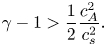 \begin{equation} \gamma - 1 > \frac{1}{2} \frac{c_A^2}{c_s^2}. \end{equation}
Note that, according to Newcomb's energy criterion (see (1.4)), for the particular atmosphere considered here, two-dimensional interchange modes ( $k_y \equiv 0$) are never unstable since the gradient of $B/\rho$ is negative. For two-dimensional undular modes ( $k_x \equiv 0$), the stability criterion is
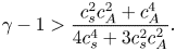 \begin{equation} \gamma - 1 > \frac{c_s^2 c_A^2 + c_A^4}{4 c_s^4 + 3 c_s^2 c_A^2}. \end{equation}
This is precisely the condition given by Parker (Reference Parker1966) (his equation (7) in the absence of cosmic ray pressure).
4.2. Anelastic case
The background state in the anelastic case is described by
 \begin{equation} \bar{\rho} =\rho_r \exp\left( \frac{z}{\bar{H}} \right), \quad \bar{p} = p_r \exp\left( \frac{z}{\bar{H}} \right), \quad \bar{T} = T_r, \quad B_0 = \tilde{B}_r \exp\left( \frac{z}{2\bar{H}} \right) , \end{equation}
where the (hydrostatic) scale height  $\bar {H}$ satisfies
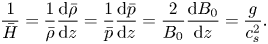 \begin{equation} \frac{1}{\bar{H}} = \frac{1}{ \bar{\rho}} \frac{\mathrm{d} \bar{\rho}}{\mathrm{d} z} = \frac{1}{\bar{p}} \frac{\mathrm{d} \bar{p}}{\mathrm{d} z} = \frac{2}{B_0} \frac{\mathrm{d} B_0}{\mathrm{d} z} = \frac{g}{c_s^2}. \end{equation}
For such a reference state, the departure from adiabaticity, defined by (2.13), is
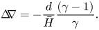 \begin{equation} \Delta\!\!{\nabla} ={-} \frac{d}{\bar{H}} \frac{(\gamma - 1)}{\gamma} . \end{equation}
For this particular atmosphere, the stratification is near adiabatic, i.e.  $\varepsilon = \left | \Delta\!\!\nabla \right | \ll 1$, when $\gamma$ is close to 1. The (sub-adiabatic) reference state entropy gradient is given by
 \begin{equation} \frac{\mathrm{d} \bar{s}}{\mathrm{d} z} ={-} \frac{c_p}{d} . \end{equation}
An important consequence of the restriction  $\gamma \cong 1$ is that the basic-state entropy gradient $\mathrm {d} s_0/\mathrm {d}z$, defined by (3.16), is ${O}(\varepsilon )$ smaller than the reference state entropy gradient $\mathrm {d} {\bar s}/\mathrm {d}z$, and hence does not enter the linearised entropy equation (3.25).
In a similar fashion to the compressible case, the linearised anelastic equations (the dimensional versions of (3.18)–(3.24)) can be combined to yield a single second-order ODE for  $\hat {w}$, with a solution of the form $\hat {w} \propto \exp \left ( -z/2\bar {H} \right ) \sin \left ( k_z z \right )$. The resulting dispersion relation for the anelastic system is
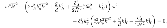 \begin{align} &- \tilde{\omega}^4 \overline{k'}^2 + \left( 2\tilde{c}_A^2 k_y^2 \overline{k'}^2 + \frac{g }{d} k_H^2 + \frac{\tilde{c}_A^2}{2\bar{H}^2}(2k_x^2 - k_H^2) \right) \tilde{\omega}^2 \nonumber\\ &\qquad\hskip10pc- \tilde{c}_A^2 k_y^2 \left( \tilde{c}_A^2 k_y^2 \overline{k'}^2 + \frac{g }{d} k_H^2 - \frac{\tilde{c}_A^2}{2\bar{H}^2} k_H^2 \right) =0, \end{align}
where  $\overline {k'}^2 = k_x^2 +k_y^2 +k_z^2 + (4\bar {H}^2)^{-1}$. The dispersion relation (4.11), which is a quadratic in $\omega ^2$, thus supports two waves – the fast mode associated with the sound wave in the compressible system has been filtered out. The remaining two waves are the gravity wave (modified by the magnetic field), and the slow magneto-acoustic mode.
Stability requires that the  $\omega ^0$ term is negative. Hence, for long wavelength modes ( $k_y \to 0$), the stability criterion reduces to
 \begin{equation} \frac{d}{\bar{H}}\frac{\tilde{c}_A^2}{c_s^2} < 2. \end{equation}
This is the anelastic version of the condition given by Yu (Reference Yu1965) for the compressible case. In fact, the anelastic condition (4.12) can be recovered from the compressible condition (4.5) by setting  $\gamma = 1+ \varepsilon (\bar {H}/d)$ and $c_A^2 = \varepsilon \tilde {c}_A^2$. Similarly, the stability criterion for two-dimensional undular modes (4.6) reduces in the anelastic case to
 \begin{equation} \frac{d}{\bar{H}}\frac{\tilde{c}_A^2}{c_s^2} < 4. \end{equation}
4.3. Comparison of the two systems
Although the derivation of the dispersion relations (4.4) and (4.11), individually, is performed most clearly in dimensional variables, it is more instructive, when comparing the two, to work with dimensionless quantities. On scaling length with the layer depth  $d$, and time with $d/c_{s}$ (i.e. $\omega \to \left ( c_{s}/d \right ) \omega$, $k \to d^{-1} k$), the compressible dispersion relation (4.4) becomes
 \begin{align} &\omega^6 - \left( \gamma k'^2 + M_A^2 (k'^2 +k_y^2) \right) \omega^4\nonumber\\ &\quad + \left( M_A^2 k_y^2 k'^2 (2\gamma + M_A^2) + (\gamma-1) \lambda^2 k_H^2 + \frac{ \lambda M_A^2}{2H} \left( 2k_x^2 - \gamma k_H^2 \right) \right) \omega^2\nonumber\\ & \hskip10pc\quad - M_A^2 k_y^2 \left( \gamma M_A^2 k_y^2 k'^2 + (\gamma-1) \lambda^2 k_H^2 - \frac{\gamma \lambda M_A^2 }{2H} k_H^2 \right) = 0, \end{align}
with dimensionless scale height  $H = \lambda ^{-1} \left ( 1+ \frac {1}{2}{M}_A^2 \right )$.
Similarly, the anelastic dispersion relation (4.11) in dimensionless form is
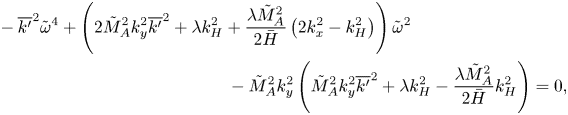 \begin{align} &- \overline{k'}^2 \tilde{\omega}^4 + \left( 2\tilde{M}_A^2 k_y^2 \overline{k'}^2 + \lambda k_H^2 + \frac{\lambda \tilde{M}_A^2}{2 \bar{H}} \left( 2k_x^2 - k_H^2 \right) \right) \tilde{\omega}^2 \nonumber\\ &\hskip10pc\quad \ - \tilde{M}_A^2 k_y^2 \left( \tilde{M}_A^2 k_y^2 \overline{k'}^2 + \lambda k_H^2 - \frac{\lambda \tilde{M}_A^2}{2 \bar{H}} k_H^2 \right) = 0, \end{align}
where  $\bar {H} = \lambda ^{-1}$. To compare directly the dispersion relation for the compressible system (4.14) with that for the anelastic system (4.15), the following additional rescaling is necessary: $\omega = \varepsilon ^{1/2} \tilde {\omega }$, $M_A = \varepsilon ^{1/2} \tilde {M}_A$. Furthermore, the restriction that the stratification of the atmosphere be close to adiabatic pins down the value of $\gamma$ (cf. (4.9)) as
 \begin{equation} \gamma = \frac{\lambda}{\lambda - \varepsilon} = 1+ \frac{\varepsilon}{\lambda} + {O}(\varepsilon^2). \end{equation}
On substitution for  $\omega$, $M_A$ and $\gamma$, (4.14) may be expressed as the following asymptotic expression:
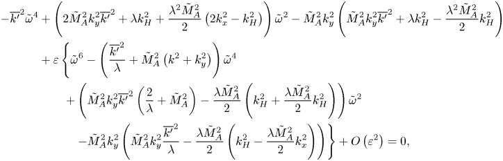 \begin{align} - \overline{k'}^2 \tilde{\omega}^4 &+ \left( 2\tilde{M}_A^2 k_y^2 \overline{k'}^2 + \lambda k_H^2 + \frac{\lambda^2 \tilde{M}_A^2}{2 } \left( 2k_x^2 - k_H^2 \right) \right) \tilde{\omega}^2 - \tilde{M}_A^2 k_y^2 \left( \tilde{M}_A^2 k_y^2 \overline{k'}^2 + \lambda k_H^2 - \frac{\lambda^2 \tilde{M}_A^2}{2 } k_H^2 \right)\nonumber\\ &+ \varepsilon \left\lbrace \tilde{\omega}^6 - \left( \frac{\overline{k'}^2}{\lambda} + \tilde{M}_A^2 \left( k^2 +k_y^2 \right) \right) \tilde{\omega}^4 \right. \nonumber\\ &\qquad\left. + \left( \tilde{M}_A^2 k_y^2 \overline{k'}^2 \left( \frac{2}{\lambda} + \tilde{M}_A^2 \right) - \frac{\lambda \tilde{M}_A^2}{2 } \left( k_H^2 + \frac{\lambda \tilde{M}_A^2}{2} k_H^2 \right) \right) \tilde{\omega}^2 \right. \nonumber\\ &\qquad\quad \left. - \tilde{M}_A^2 k_y^2 \left( \tilde{M}_A^2 k_y^2 \frac{\overline{k'}^2}{\lambda} - \frac{ \lambda \tilde{M}_A^2 }{2} \left( k_H^2 - \frac{\lambda \tilde{M}_A^2}{2} k_x^2 \right) \right) \right\rbrace + {O}\left( \varepsilon^2 \right) =0, \end{align}
where  $k^2 = k_x^2 + k_y^2 + k_z^2$. Setting $\varepsilon = 0$ in (4.17) recovers the anelastic dispersion relation (4.15). By inspecting the expression (4.17), we can assess under what conditions do the dispersion relations resulting from the compressible and anelastic systems produce significantly different results. In particular, we are interested in seeing if there are circumstances under which the asymptotic ordering can be broken, with terms that are formally ${O}\left ( \varepsilon \right )$ being ‘promoted’ to ${O}\left ( 1 \right )$.
For any of the  ${O}\left ( \varepsilon \right )$ terms (in curly brackets) to come into play at ${O}\left ( 1 \right )$, $\tilde {M}_A^2$ would have to be as large as ${O}\left ( \varepsilon ^{-1} \right )$ – a value far beyond the regime of validity of the anelastic approximation; with this ordering, the Alfvén wave speed would be comparable to the speed of sound, and the magnetic field would be strong enough to upset the assumed hydrostatic balance at leading order. At first glance one might also intuit that some of the ${O}\left ( \varepsilon \right )$ terms could contribute to the dominant balance if $\lambda \sim \varepsilon$. However, the derivation of (4.17) involves expanding $\gamma$ according to (4.16) which is valid only for $\lambda \gg \varepsilon$. The validity of the expression (4.17) requires that $\tilde {M}_A^2$ be of order unity and $\varepsilon /\lambda \ll 1$ – under these restrictions it is not possible to upset the ${O}(\varepsilon ^0)$ balance.
Figure 1 compares (squared) frequencies of the slow magneto-acoustic mode for a range of wavenumbers  $k_x$, $k_y$ and increasing values of $\tilde {M}_A^2$. Positive (negative) values correspond to stability (instability). As for all diffusionless magnetic buoyancy instabilities (see, for example, the energy principle analysis of Hughes & Cattaneo Reference Hughes and Cattaneo1987), instability is favoured for large $k_x$ and small $k_y$. As expected, qualitative and quantitative agreement between the two systems is very good when $\tilde {M}_A^2 = 10$. The agreement between the two systems worsens as $\tilde {M}_A^2$ is increased. When $\tilde {M}_A^2 = 50$, quantitative agreement is less good, but the overall features of the contour plot are still captured by the anelastic system. When $\tilde {M}_A^2$ is as large as $\varepsilon ^{-1}$, in this case $\tilde {M}_A^2 = 100$, the agreement between compressible and anelastic systems breaks down and there are large differences between the solutions of the two systems.
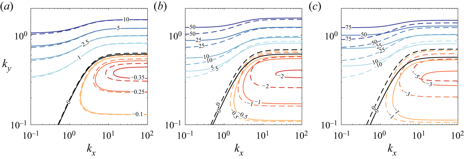
Figure 1. Contours of the (squared) frequency  $\tilde {\omega }^2$ of the slow magneto-acoustic mode for the compressible system, with $\varepsilon = 0.01$ (solid lines), and the anelastic system (dashed lines); $\lambda =1$, $k_z = {\rm \pi}$. In (a) $\tilde {M}_A^2=10$; in (b) $\tilde {M}_A^2=50$; in (c) $\tilde {M}_A^2=100$.
5. Instabilities of more general equilibria
In § 4 we examined the instabilities of an isothermal atmosphere with constant Alfvén speed; this particular choice allows an analytical solution and hence a detailed comparison of the compressible and anelastic systems. In this section, we extend our study to consider the instabilities of two other magnetohydrostatic atmospheres, again with the aim of comparing results obtained under the anelastic approximation with those from the full system. As noted earlier, the eigenvalue problem determining the linear growth rate requires, in general, a numerical solution.
5.1. Isothermal atmosphere with linear magnetic stratification
Here, as in § 4, we again consider an isothermal atmosphere, but now with the magnetic field linearly stratified with depth. The equilibrium temperature and magnetic field distributions are given by
 \begin{equation} T_b = \bar{T} = 1, \quad B_b = B_0 = 1 + \zeta z . \end{equation}
From (3.3), the basic-state density in the compressible system is then given by
 \begin{equation} \rho_b(z) = p_b(z) = \exp( \lambda z) \left\lbrace 1 + \frac{ \zeta M_A^2 }{ \lambda } \left[ \zeta z \exp(-\lambda z) - \left( 1 + \frac{\zeta}{\lambda} \right) \left( 1- \exp(-\lambda z) \right) \right] \right\rbrace . \end{equation}
In the anelastic system, the non-magnetised reference state is described by
 \begin{equation} \bar{\rho}(z) = \bar{p}(z) = \exp( \lambda z), \quad \frac{\mathrm{d} \bar{s}}{\mathrm{d} z} ={-}1. \end{equation}
Recall that the departure from adiabaticity  $\varepsilon$ for an isothermally stratified atmosphere is governed by (4.9). Thus, in the compressible system, a subadiabatic value of $\gamma$ is chosen according to $\gamma = \lambda /(\lambda - \varepsilon )$. In the anelastic system, we use the value of $\gamma$ that gives exactly adiabatic stratification, i.e. $\gamma _{ad} = 1$. As a consequence, the basic state entropy gradient does not enter the picture (i.e. $\mathrm {d} s_0/ \mathrm {d}z = 0$).
Figure 2 shows the growth rate of the magnetic buoyancy instability as a function of  $\tilde {M}_A^2$ for various magnetic field gradients $\zeta$ and various degrees of departure of adiabaticity $\varepsilon$, for fixed $k_x = 4$, $k_y = 0.01$, $\lambda = 1$. Since our interest lies in comparison of the anelastic and compressible systems, rather than in an extensive investigation of the instability, we have concentrated on fixed values of the wavenumbers, but recognising the fact that the instability mechanism is favoured when $k_y \ll k_x$.
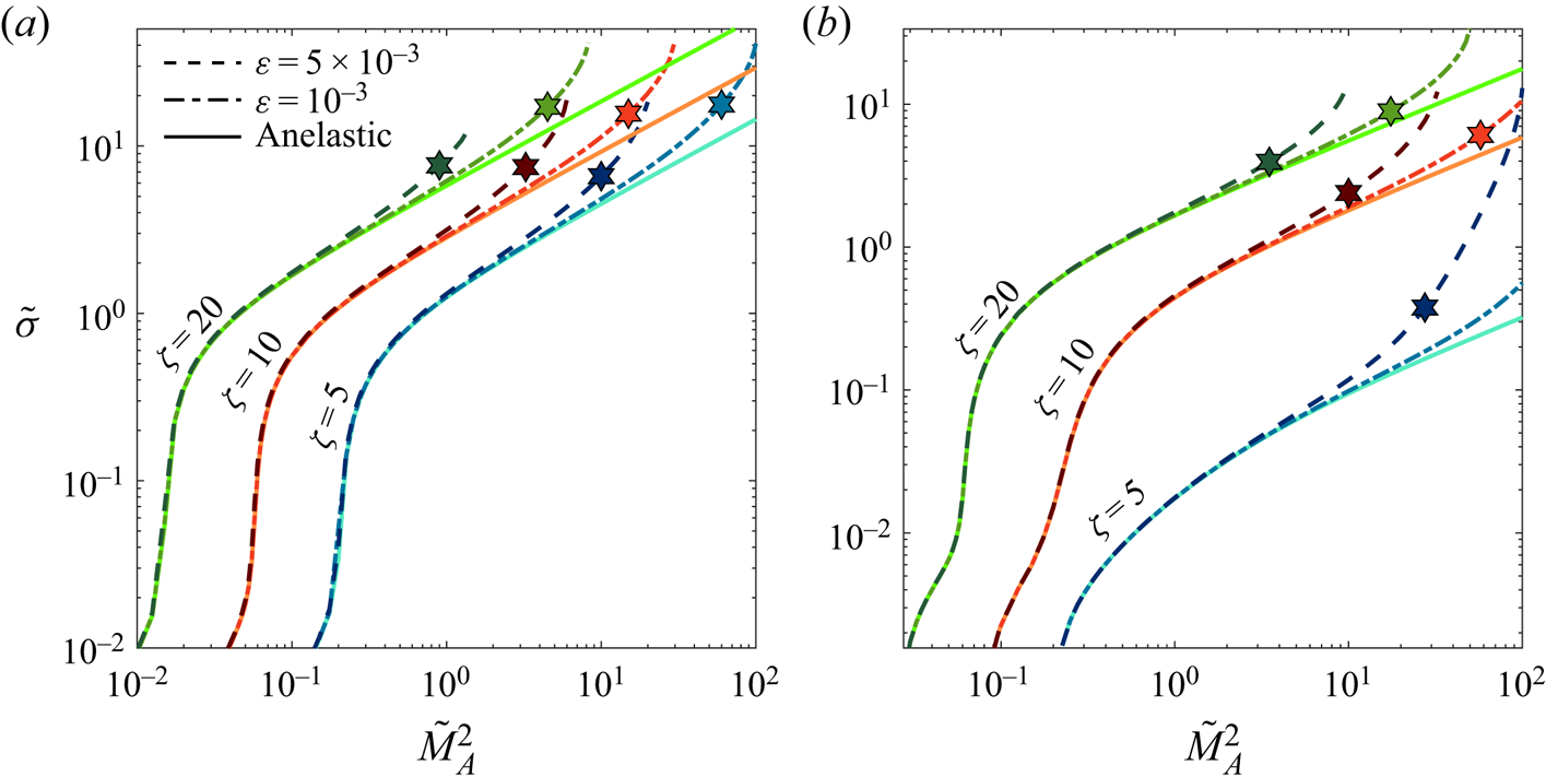
Figure 2. Growth rates  $(\tilde \sigma = -{\rm Im}(\tilde{\omega}))$ of magnetic buoyancy instability in compressible ( $\varepsilon =10^{-3}\ \text{and} \varepsilon = 5 \times 10^{-3}$) and anelastic systems as a function of $\tilde {M}_A^2$, for various field gradients ( $\zeta =5, 10, 20$). In (a) $\lambda =1$; in (b) $\lambda =5$. Stars denote the positions where $G_{max} = 0.7/\varepsilon$.
For a given value of  $\zeta$, the agreement between the compressible and anelastic results improves as $\varepsilon$ is reduced. This is expected and reassuring. For a given $\varepsilon$ and $\tilde {M}_A^2$, the discrepancy between the two systems becomes larger as $\zeta$ is increased. In the case of the compressible system, the basic state can be substantially altered by the presence of the strong field gradient (large $\zeta$); i.e. magnetic stratification can provide a significant contribution to the background entropy gradient. The basic-state entropy gradient (3.27) can be thought of as a sum of atmospheric gradient $\beta ^A$ and magnetic gradient $\beta ^M$ contributions, $\mathrm {d} s_b/ \mathrm {d}z = \beta ^A + \beta ^M$. For this particular nearly adiabatic basic state, the atmospheric contribution is $\left | \beta ^A \right | = \varepsilon$, and the magnetic part is, to leading order, $\beta ^M = \varepsilon ^2 G/\lambda$, where $G = \tilde {M}_A^2 \zeta B_0/\bar {p}$. In the anelastic system, the corresponding part of the entropy gradient due to magnetic stratification does not enter the governing equations ( $\mathrm {d} s_0/ \mathrm {d}z = 0$). This difference between the two systems does not result in a significant disagreement between them provided that $G = {O}(1)$; in this case, the background entropy gradient is, to leading order ( ${O}(\varepsilon )$), given by the atmospheric gradient $\beta ^A$, and the magnetic component $\beta ^M$ is ${O}(\varepsilon ^2)$. However, we can expect breakdown of the agreement between the two systems when the magnetic part of the entropy gradient – which does not enter the picture in the anelastic system – becomes large enough to be influential in the compressible system, i.e. when $\beta ^M = {O}(\varepsilon )$. This requires $G={O}(\varepsilon ^{-1})$. The maximum value of $G$ in the interval $0 \leqslant z \leqslant 1$ is
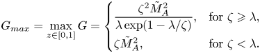 \begin{equation} G_{max} = \max_{z \in [0,1]} G = \left\{\begin{array}{@{}ll} \dfrac{ \zeta^2 \tilde{M}_A^2}{\lambda \exp(1-\lambda/\zeta)}, & \text{for } \zeta \geqslant \lambda, \\ \zeta \tilde{M}_A^2 , & \text{for } \zeta < \lambda. \end{array}\right. \end{equation}
Thus we can expect breakdown of the agreement between the two systems when  $G_{max}$ becomes as large as $1/\varepsilon$; i.e. the validity of the anelastic approximation can be broken by a large enough field gradient $\zeta = {O}(\varepsilon ^{-1/2})$, even if the field is weak $\tilde {M}_A^2 = {O}(1)$. The argument above is confirmed in figure 2, where we mark values of $\tilde {M}_A^2$ for which $G_{max} = 0.7/\varepsilon$.
5.2. Linear temperature and magnetic stratification
Now we consider the case where the equilibrium temperature and magnetic field distributions are given by
 \begin{equation} T_b =\bar{T}= 1 + \theta z, \quad B_b = B_0 = 1 + \zeta z. \end{equation}
The basic-state density in the compressible system is (from (3.3))
 \begin{equation} \rho_b(z) = \left( 1+\theta z \right)^m \left\lbrace 1 - \zeta M_A^2 \frac{\left( \zeta + (m-1)\theta \right)\left[ (1+\theta z)^m - 1 \right] - m\zeta \theta z }{ m(m-1)\theta^2 (1+\theta z)^m }\right\rbrace, \end{equation}
where  $m = (\lambda /\theta - 1)$ is the polytropic index. The basic-state pressure is $p_b = \rho _b T_b$. In the anelastic system, the non-magnetised reference state density and pressure take the form of polytropes,
 \begin{equation} \bar{\rho} = \left( 1+\theta z \right)^{m}, \quad \bar{p} = \left( 1+\theta z \right)^{m+1}. \end{equation}
The departure from adiabaticity for such an atmospheric stratification is given by
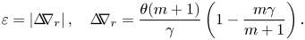 \begin{equation} \varepsilon = \left| \Delta\!\!{\nabla}_r \right|, \quad \Delta\!\!{\nabla}_r = \frac{\theta (m+1)}{\gamma} \left( 1 - \frac{m \gamma}{m+1} \right) . \end{equation}
For a given  $\gamma$, the polytropic index corresponding to adiabatic stratification is $m_{ad} = 1/(\gamma - 1)$. For the isothermal atmospheres discussed in §§ 4 and 5.1, the constraint of near adiabaticity required $\gamma$ to be close to unity; here, the value of $\gamma$ is unrestricted, so we adopt the standard value of $\gamma =5/3$. In the compressible system, with temperature stratification $\theta$, $\varepsilon$ is adjusted by selecting the appropriate polytropic index $m$, according to (5.8a,b). In the anelastic case we take the value of $m$ that gives exactly adiabatic stratification; with $\gamma =5/3$, $m_{ad} = 1.5$. The sub-adiabatic reference state entropy gradient is given by
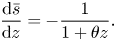 \begin{equation} \frac{\mathrm{d} \bar{s}}{\mathrm{d} z} ={-} \frac{1}{1+ \theta z}. \end{equation}
Note that, in contrast to the isothermal atmospheres, where the basic state entropy gradient does not enter the anelastic equations, here, it does come into play.
Figure 3 compares the growth rates of the magnetic buoyancy instability between the compressible and anelastic systems, again with  $k_x = 4$, $k_y = 0.01$. The agreement between the two systems is better for larger stratification $\theta$.

Figure 3. Growth rates  $(\tilde \sigma = -{\rm Im}(\tilde{\omega}))$ of magnetic buoyancy instability in compressible ( $\varepsilon =10^{-3}$ and $\varepsilon = 5 \times 10^{-3}$) and anelastic systems as a function of $\tilde {M}_A^2$ for the case of equilibria with linear temperature and magnetic field stratification ( $\zeta =5, 10, 20$). In (a) $\theta =5$; in (b) $\theta =20$. Stars denote the positions where $H_{max} = 0.7/\varepsilon$.
The anelastic system is formally valid when the magnetic contribution to the entropy gradient  $\mathrm {d} s_0/ \mathrm {d}z$ is order unity. We have seen above how, through a combination of large field strength and strong field gradient, the magnetic field can substantially affect the background entropy gradient. Here, it is also true that for sufficiently large $\tilde {M}_A^2$ and $\zeta$, the basic-state entropy gradient can become as large as $\mathrm {d} s_0/ \mathrm {d}z = {O}(\varepsilon ^{-1})$. In this case, the formal asymptotic ordering is broken, and the influence of magnetic field is strong enough to modify the assumed hydrostatic equilibrium. The maximum value of $\mathrm {d} s_0/ \mathrm {d}z$ in the interval $0 \leqslant z \leqslant 1$ is
 \begin{equation} H_{max} = \max_{z \in [0,1]} \frac{\mathrm{d} s_0}{\mathrm{d} z} = \left\{\begin{array}{@{}ll} \dfrac{(\gamma-1)}{\gamma} \dfrac{ \zeta (\zeta - \theta) \tilde{M}_A^2}{ (\gamma(1-\theta/\zeta) )^{m_{ad}+1}}, & \text{for } \zeta \geqslant (m_{ad}+1)\theta, \\ \dfrac{(\gamma-1)}{\gamma} \zeta \tilde{M}_A^2 , & \text{for } \zeta < (m_{ad}+1)\theta. \end{array}\right. \end{equation}
Thus we anticipate breakdown of the asymptotic ordering, and hence a breakdown of the agreement between the results of the compressible and anelastic systems, when  $H_{max}$ becomes as large as $1/\varepsilon$. For illustration, in figure 3, we mark the values of $\tilde {M}_A^2$ for which $H_{max} = 0.7/\varepsilon$.
6. A note on the energy principle of ideal MHD
One of the most elegant and widely used means of analysing the linear stability of ideal, compressible MHD equilibria is via the energy principle of Bernstein et al. (Reference Bernstein, Frieman, Kruskal and Kulsrud1958). The underlying idea is to express the change in potential energy  $\delta W$ resulting from a Lagrangian displacement $\boldsymbol{\xi }$ as an integral, involving $\boldsymbol{\xi }$ and its spatial derivatives, together with the basic-state distributions of pressure, density and magnetic field. It is then possible readily to formulate necessary conditions for instability; furthermore – thus making the energy principle particularly powerful – it is often possible, owing to the self-adjointness of the force operator, to deduce sufficient conditions for instability. In the light of the preceding discussions, it is therefore of interest to formulate the corresponding energy principle for anelastic MHD, with particular emphasis on its description of magnetic buoyancy instability. In this context, the energy principle for anelastic MHD has also previously been addressed by Fan (Reference Fan2001), although from a slightly different perspective to that taken here.
Within the constraints of the anelastic approximation, we first consider a general magnetohydrostatic equilibrium. As in § 2.2, we denote the reference state variables by an overbar, and, as in § 3.2, basic-state variables by a subscript ‘0’; also as in § 2.2, we express perturbations to the basic state by  $\boldsymbol{\delta u}^*$, $\boldsymbol{\delta b}^*$, $\delta s^*$, etc. The linearised forms of (2.22), (2.32), (2.24) and (2.25) may then be written as
 \begin{gather} \boldsymbol{\nabla}\boldsymbol{\cdot} \left( \bar{\rho} \, \boldsymbol{ \delta u}^* \right) = 0, \end{gather}
 \begin{gather}\frac{\partial \boldsymbol{\delta u}^*}{\partial t^*} ={-} \boldsymbol{\nabla} \left( \frac{\delta p^*}{\bar{\rho}} \right) - \frac{\delta s^*}{c_p} \boldsymbol{ g } + \frac{1}{\mu_0 \bar{\rho}} \left( \boldsymbol{\nabla}\times \boldsymbol{B}_0 \right) \times \boldsymbol{ \delta b }^* + \frac{1}{\mu_0 \bar{\rho}} \left( \boldsymbol{\nabla}\times \boldsymbol{\delta b}^* \right) \times \boldsymbol{B}_0, \end{gather}
 \begin{gather}\frac{\partial \boldsymbol{\delta b}^*}{\partial t^*} = \boldsymbol{\nabla}\times \left( \boldsymbol{ \delta u}^* \times \boldsymbol{B}_0 \right), \end{gather}
 \begin{gather}\frac{\partial \delta s^*}{\partial t^*} + \boldsymbol{\delta u}^* \boldsymbol{\cdot} \boldsymbol{\nabla} \left( \bar{s}+s_0 \right)= 0. \end{gather}
Under the linear approximation, the fluid velocity  $\boldsymbol{ \delta u}^*$ is linked to the Lagrangian displacement $\boldsymbol{\xi }$ through the simple relation
 \begin{equation} \boldsymbol{ \delta u}^* = \frac{\partial \boldsymbol{\xi}}{\partial t^*}. \end{equation}
Integrating (6.1), (6.3) and (6.4) with respect to time thus gives
 \begin{gather} \boldsymbol{\nabla}\boldsymbol{\cdot} \left( \bar{\rho} \boldsymbol{\xi} \right) = 0, \end{gather}
 \begin{gather}\boldsymbol{\delta b}^* = \boldsymbol{\nabla}\times \left( \boldsymbol{\xi} \times \boldsymbol{B}_0 \right), \end{gather}
 \begin{gather}\delta s^* ={-} \boldsymbol{\xi} \boldsymbol{\cdot} \boldsymbol{\nabla} \left( \bar{s}+s_0 \right). \end{gather}
The momentum equation (6.2) can be expressed formally as
 \begin{equation} \bar{\rho} \frac{ \partial^2 \boldsymbol{\xi}}{\partial t^{*2} } = \boldsymbol{F} (\boldsymbol{\xi} ), \end{equation}
where the force operator  $\boldsymbol{F}$ is defined by
 \begin{equation} \boldsymbol{F} (\boldsymbol{\xi}) ={-} \bar{\rho} \boldsymbol{\nabla} \left( \frac{\delta p^*}{\bar{\rho}} \right) - \frac{\delta s^* \bar \rho}{c_p} \boldsymbol{ g } + \frac{1}{\mu_0 } \left( \boldsymbol{\nabla}\times \boldsymbol{B}_0 \right) \times \boldsymbol{\delta b}^* + \frac{1}{\mu_0 } \left( \boldsymbol{\nabla}\times \boldsymbol{ \delta b}^* \right) \times \boldsymbol{B}_0. \end{equation}
As with the expression for  $\boldsymbol{F}$ for fully compressible MHD, it is straightforward although tedious to establish that $\boldsymbol{F}$ is self-adjoint.
The change in potential energy  $\delta W$ over the fluid volume $V$ is given by
 \begin{equation} \delta W ={-}\tfrac{1}{2} \int _V \boldsymbol{\xi} \boldsymbol{\cdot} \boldsymbol{F} (\boldsymbol{\xi} ) \, \mathrm{d} V. \end{equation}
On substituting for  $\boldsymbol{F}$ from (6.10), making use of standard integral manipulations and the boundary condition that $\boldsymbol{\xi } \boldsymbol {\cdot } \boldsymbol{n} =0$ on the boundary of $V$, and substituting from (6.7) and (6.8), we obtain
 \begin{equation} \delta W = \frac{1}{2} \int_V \left\{ \frac{1}{\mu_0} \left| \boldsymbol{\nabla}\times \left( \boldsymbol{\xi} \times \boldsymbol{B}_0 \right) \right|^2 - \boldsymbol{j}_0 \boldsymbol{\cdot} \left( \left( \boldsymbol{\nabla} \times (\boldsymbol{\xi} \times \boldsymbol{B}_0) \right) \times \boldsymbol{\xi} \right) - \frac{\bar{\rho}}{c_p} \left( \boldsymbol{\xi} \boldsymbol{\cdot} \boldsymbol{g} \right) \boldsymbol{\xi} \boldsymbol{\cdot} \boldsymbol{\nabla} \left( \bar{s}+s_0 \right) \right\} {\rm d}V, \end{equation}
where  $\boldsymbol{j}_0 = \mu _0^{-1} \boldsymbol{\nabla }\times \boldsymbol{B}_0$. Expression (6.12), which is an integral of a quadratic expression for $\boldsymbol{\xi }$ and its first derivatives, with coefficients governed by the basic state, is the general expression for $\delta W$ under the anelastic approximation. For the magnetohydrostatic atmospheres considered in this paper, with $\boldsymbol{B}_0=B_0(z) \hat {\boldsymbol{y}}$ and $\boldsymbol{g} = g \hat {\boldsymbol{z}}$, (6.12) becomes
 \begin{align} &\delta W = \frac{1}{2} \int_V \left\{ \frac{B_0^2}{\mu_0} \left[ \left( \frac{\partial \xi_x}{\partial y} \right)^2 + \left( \frac{\partial \xi_z}{\partial y} \right)^2 + \left( \frac{\partial \xi_x}{\partial x} + \frac{\partial \xi_z}{\partial z} \right)^2 \right] \right. \nonumber\\ &\hskip10pc\quad \left.\vphantom{\left[ \left( \frac{\partial \xi_x}{\partial y} \right)^2 + \left( \frac{\partial \xi_z}{\partial y} \right)^2 + \left( \frac{\partial \xi_x}{\partial x} + \frac{\partial \xi_z}{\partial z} \right)^2 \right] }+ \frac{B_0}{\mu_0} \frac{\mathrm{d} B_0}{\mathrm{d} z} \left( \boldsymbol{\nabla}\boldsymbol{\cdot} \boldsymbol{\xi} \right) \xi_z - \frac{\bar{\rho} g}{c_p} \frac{\mathrm{d} }{\mathrm{d} z} \left( \bar{s}+s_0 \right) \xi_z^2 \right\} \,{\rm d}V. \end{align}
Seeking solutions of the form
 \begin{equation} \boldsymbol{\xi} = \left( {\hat \xi_x}(z) \sin k_x x \sin k_y y, \, {\hat \xi_y}(z) \cos k_x x \cos k_y y, \, {\hat \xi_z}(z) \cos k_x x \sin k_y y \right), \end{equation}
gives, after substituting for  $\boldsymbol{\nabla } \boldsymbol {\cdot } \boldsymbol{\xi }$ from (6.6) and dropping hats,
 \begin{align} &\hskip-4pc\delta W = \frac{1}{8} \int_V \left\{ \frac{B_0^2}{\mu_0} \left[ k_y^2 \left( \xi_x^2 + \xi_z^2 \right) + \left( k_x \xi_x + \xi_z' \right)^2 \right] \right. \nonumber\\ &\quad\quad \left. + \frac{B_0}{\mu_0} \frac{\mathrm{d} B_0}{\mathrm{d} z} \left( k_x \xi_x - k_y \xi_y + \xi_z' \right) \xi_z - \frac{\bar{\rho} g}{c_p} \frac{\mathrm{d} }{\mathrm{d} z} \left( \bar{s}+s_0 \right) \xi_z^2 \right\} {\rm d}z, \end{align}
where  $'$ denotes differentiation with respect to z. It is instructive to compare (6.15) with the corresponding expression for compressible MHD (see Hughes & Cattaneo Reference Hughes and Cattaneo1987), which we shall denote by $\delta W_{\mathrm {comp}}$, where
 \begin{align} \delta W_{{comp}} &= \frac{1}{8} \int_V \left\{ \frac{B_b^2}{\mu_0} \left[ k_y^2 \left( \xi_x^2 + \xi_z^2 \right) + \left( k_x \xi_x + \xi_z' \right)^2 \right] \right. + \gamma p_b \left( k_x \xi_x - k_y \xi_y + \xi_z' \right)^2\nonumber\\ &\quad\quad\qquad \left.\vphantom{\frac{B_b^2}{\mu_0}}+ 2 \rho_b g \left( k_x \xi_x - k_y \xi_y + \xi_z' \right) \xi_z + g \rho_b' \xi_z^2 \right\} {\rm d}z. \end{align}
As shown by Hughes & Cattaneo (Reference Hughes and Cattaneo1987), for the case of fully compressible MHD, expressions (1.4) and (1.5) follow by minimising  $\delta W_{\mathrm {comp}}$ over the components of $\boldsymbol{\xi }$. For anelastic MHD, the situation is slightly different, in that $\delta W$, given by (6.15), must be minimised subject to the constraint provided by (6.6).
For interchange modes ( $k_y=0$), the $\xi _x$ term appears only in the combination $( k_x \xi _x + \xi _z' )$, which represents $\boldsymbol{\nabla } \boldsymbol {\cdot } \boldsymbol{\xi }$. Using (6.6) one further time thus gives
 \begin{equation} \delta W = \frac{1}{8} \int_V \left( \frac{B_0^2}{\mu_0} \left( \frac{{\bar{\rho}}'}{{\bar{\rho}}} \right)^2 - \frac{B_0}{\mu_0} \frac{\mathrm{d} B_0}{\mathrm{d} z} \frac{{\bar{\rho}}'}{{\bar{\rho}}} - \frac{\bar{\rho} g}{c_p} \frac{\mathrm{d} }{\mathrm{d} z} \left( \bar{s}+s_0 \right) \right) \xi_z^2 \, {\rm d}z. \end{equation}
Pursuing the same line of argument as for the energy principle of compressible MHD, it therefore follows that a necessary and sufficient condition for instability is that the inequality
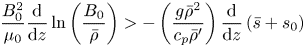 \begin{equation} \frac{B_0^2}{\mu_0} \frac{\mathrm{d}}{\mathrm{d}z} \ln \left( \frac{B_0}{\bar \rho}\right) >{-} \left( \frac{g {\bar \rho}^2 }{c_p {\bar \rho}'} \right) \frac{\mathrm{d} }{\mathrm{d} z} \left( \bar{s}+s_0 \right) \end{equation}
holds somewhere in the fluid. Criterion (6.18) is in agreement with that obtained by taking the anelastic limit of the general interchange instability criterion (1.4). It is of interest to note that, whereas for the compressible system, the instability criterion for interchange modes requires minimisation over  $( k_x \xi _x + \xi _z' )$, no such minimisation is required, or even possible, in the anelastic system; instead, $( k_x \xi _x + \xi _z' )$ is constrained through the mass conservation equation (6.6).
For three-dimensional modes ( $k_x \ne 0$, $k_y \ne 0$), we incorporate the constraint (6.6) through substitution into (6.15) to obtain
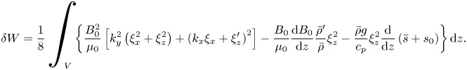 \begin{equation} \delta W = \frac{1}{8} \int_V \left\{ \frac{B_0^2}{\mu_0} \left[ k_y^2 \left( \xi_x^2 + \xi_z^2 \right) + \left( k_x \xi_x + \xi_z' \right)^2 \right] - \frac{B_0}{\mu_0} \frac{\mathrm{d} B_0}{\mathrm{d} z}\frac{{\bar{\rho}}'}{{\bar{\rho}}} \xi_z^2 -\frac{\bar{\rho} g}{c_p} \xi_z^2 \frac{\mathrm{d} }{\mathrm{d} z} \left( \bar{s}+s_0 \right) \right\} {\rm d}z. \end{equation}
As discussed by Hughes & Cattaneo (Reference Hughes and Cattaneo1987), the most unstable modes are those that are solenoidal in the plane perpendicular to the imposed field and, in addition, have  $k_y \to 0$. A necessary and sufficient criterion for instability is then that
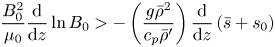 \begin{equation} \frac{B_0^2}{\mu_0} \frac{\mathrm{d}}{\mathrm{d}z} \ln B_0 >{-} \left( \frac{g {\bar \rho}^2 }{c_p {\bar \rho}'} \right) \frac{\mathrm{d} }{\mathrm{d} z} \left( \bar{s}+s_0 \right) \end{equation}
holds somewhere in the fluid. Criterion (6.20) is in agreement with that obtained by taking the anelastic limit of the general criterion for three-dimensional instability (1.5).
7. Conclusions and discussion
To aid theoretical and computational studies of compressible fluid dynamics it is often helpful to apply some simplifying assumptions to the governing equations of compressible MHD in order to derive a simpler, asymptotically consistent reduced system. Indeed, magnetic buoyancy has been studied using the reduced ‘magneto-Boussinesq’ equations derived by Spiegel & Weiss (Reference Spiegel and Weiss1982) and Corfield (Reference Corfield1984). More recently, Bowker et al. (Reference Bowker, Hughes and Kersalé2014) developed a distinct set of magneto-Boussinesq equations that allowed for the study of magnetic buoyancy in the presence of velocity shear. Fan (Reference Fan2001) studied the nonlinear break-up of a magnetic layer under magnetic buoyancy instability in the further distinct regime of anelastic MHD. The development of both of the aforementioned Boussinesq reduced systems requires the imposition that the characteristic length scale parallel to the direction of the imposed field is longer (in a strict asymptotic sense) than the characteristic transverse scale. The equations of anelastic MHD on the other hand involve no such constraint: no distinction is drawn between length scales parallel and perpendicular to the imposed magnetic field. The equations of anelastic MHD were originally developed to study thermal convection in the presence of an evolving magnetic field – with the notable application being the geodynamo model of Braginsky & Roberts (Reference Braginsky and Roberts1995). As such, the question of how magnetic buoyancy fits into the anelastic picture was not a primary concern. However, given the subtleties involved in incorporating the effects of magnetic buoyancy into the Boussinesq approximation, it is by no means clear, a priori, whether the phenomenon of magnetic buoyancy is faithfully represented by the equations of anelastic MHD. Motivated by this apparent conundrum, in this article we have pursued two closely related objectives. The first is to formalise the relationship between descriptions of magnetic buoyancy in the compressible, anelastic, and Boussinesq systems. The second is to assess the conditions under which the equations of anelastic MHD provide an accurate description of magnetic buoyancy instability.
Our first aim is accomplished in § 2, where, by using an order of magnitude analysis, we derive the scalings that must be obeyed to account for the effects of magnetic buoyancy. Magnetic buoyancy arises when magnetic pressure plays a role in regulating local gas density. Thus, a minimal requirement for this process to be captured in the reduced equations is that magnetic pressure fluctuations are of the same order of magnitude as density fluctuations. This requirement in turn imposes an important relation between the parallel length scale of perturbations  $L_B$, the pressure scale height $H_p$ and magnetic field scale height $H_B$, namely that $L_B \sim \sqrt {H_p H_B}$ (expression (2.44)). Magnetic buoyancy is captured within the set of reduced equations only if this relation is satisfied. In the standard anelastic approximation, both pressure and magnetic scale heights are comparable to the depth of the fluid $d$: i.e. $d \sim H_p \sim H_B$. Thus, the characteristic parallel length scale of magnetic buoyancy perturbations is comparable to the transverse length scale (layer depth): $L_B \sim d$. This explains why no special treatment of length scales is required in order to include magnetic buoyancy under the standard anelastic approximation; expression (2.44) is intrinsically satisfied within the standard anelastic approximation. Based on the orderings derived in § 2 we have identified five distinct asymptotically consistent regimes of compressible MHD. Four of these regimes satisfy (2.44) and thus include the phenomenon of magnetic buoyancy (two in the anelastic approximation and two in the Boussinesq approximation). The fifth regime is the ‘Boussinesq magnetoconvection’ regime, in which the effects of magnetic buoyancy are excluded. We describe the scalings underpinning these distinct regimes in detail in § 2.4. Furthermore, in Appendix A, we derive the governing equations in each regime by taking appropriate limits of the standard anelastic system. Our formal asymptotic approach makes the relationship between the various reduced systems fully transparent and pins down the conditions of validity of each regime. In particular, the asymptotic conditions for the validity of the anelastic MHD approximation require that both the equilibrium entropy gradient and the magnitude of the magnetic field are small, i.e. $\left | \Delta\!\!\nabla \right | \sim M_A^2 \sim \varepsilon$.
In regard to our second objective, we compare, for various magnetohydrostatic equilibria, the growth rates of the magnetic buoyancy instability in compressible MHD with those in anelastic MHD. The agreement between the two systems is in line with the theoretical (asymptotic) conditions for the validity of the anelastic approximation: provided the magnetic field gradient is not excessively large ( $d/H_B = {O} (1)$), compressible solutions converge to the anelastic ones when the stratification is nearly adiabatic ( $\left | \Delta\!\!\nabla \right | \ll 1$) and magnetic pressure is small in comparison with plasma pressure ( $M_A^2 \ll 1$). The agreement between the two systems breaks down when either of the conditions is violated. It should be noted that the agreement also fails when the field gradient is sufficiently large ( $d/H_B \gg 1$), even for weak field strengths. The requirement of near adiabaticity is most restrictive for the cases of isothermal stratification, where it restricts the validity of anelastic approximation to gases with $\gamma \cong 1$. Although this is far from the traditional value commonly adopted in studies of stellar interiors with hydrogen plasma, where $\gamma = 5/3$, it is, however, potentially relevant for interstellar thermal gas, where the effective $\gamma$ is 1 or less (Parker Reference Parker1953).
Given that the equations of anelastic MHD are most commonly used in astrophysical modelling, it is important to discuss how the conditions for validity of anelastic MHD measure up against physical reality. As a concrete example, we may consider the interior of the Sun. Departure from adiabaticity is small throughout the bulk of the convection zone;  $\Delta\!\!\nabla \lesssim 10^{-6}$ at the base of the convection zone, with stratification becoming substantially superadiabatic only near the solar surface. Below the convection zone, in the solar radiative interior, the stratification is significantly subadiabatic, with $\Delta\!\!\nabla$ of order unity. Although there is no consensus on precisely how the solar dynamo operates, it is widely believed that the bulk of the solar magnetic field resides in the tachocline, a thin shear region at the base of, or just beneath, the convection zone. While surface observations provide good measurements of the field strength at the solar surface, we have very limited knowledge of the field strength at depth. Theoretical estimates of the mean toroidal field strength in the tachocline are in the range $10^3$– $10^5$ G. When expressed in terms of the square of the Alfvén Mach number, this certainly makes the field weak: $10^{-10} \lesssim M_A^2 \lesssim 10^{-6}$. We do not expect $M_A^2$ to be larger than this throughout the majority of the convection zone, with the exception of near-surface regions where the plasma pressure becomes small and the magnetic field exists in the form of intense flux concentrations; there, magnetic pressure becomes comparable to the plasma pressure and $M_A^2$ can be of order unity. The smallness of $\Delta\!\!\nabla$ and $M_A^2$ thus makes the anelastic approximation valid in the bulk of the convection zone. There, however, the dynamics is dominated by turbulent convection, with magnetic buoyancy not expected to play a significant role. Magnetic buoyancy is, however, believed to be a key player in subadiabatic regimes, in particular being the primary candidate for the release of strong toroidal field from the interior. In the stably stratified lower tachocline, Petrovay (Reference Petrovay2003) puts forward that a useful approximation for the departure from adiabaticity is $\Delta\!\!\nabla=-0.015 z$, where $z$ is the depth below the base of the convection zone, measured in $\textrm {Mm}$. Since the width of the tachocline $h_t$, is estimated to be approximately $4\,\%$ of the solar radius ( $h_t \approx 30\ \textrm {Mm}$) (see Christensen-Dalsgaard & Thompson Reference Christensen-Dalsgaard and Thompson2007), this suggests that $|\Delta\!\!\nabla |$ remains less than unity throughout the tachocline and hence that the constraints of the anelastic approximation are indeed satisfied. In the deeper radiative interior, although magnetic pressure is expected to be a small fraction of the plasma pressure $M_A^2 \ll 1$, the stratification is strongly subadiabatic $\left | \Delta\!\!\nabla \right | \gtrsim {O}(1)$. Thus, the anelastic approximation cannot capture all of the dynamics of the solar radiative zone. Nonetheless, although not painting the entire picture, we envisage that the equations of anelastic MHD will still provide valuable insight into the dynamics of magnetic buoyancy instabilities in atmospheres that are strongly stratified in density, and thus representative of stellar interiors.
It remains to note that our considerations in this paper have excluded all effects of diffusion. The neglect of diffusion terms would not appear to be of overriding significance, in that the subtleties arising from the inclusion of magnetic fields in the various approximations do not lie in the diffusion terms. The inclusion of diffusive effects in the anelastic and magneto-Boussinesq approximations merely requires that the diffusion coefficients (viscosity, thermal and magnetic diffusivity) enter at precisely the order at which they play an active, but not dominant, role (Corfield Reference Corfield1984; Lantz & Fan Reference Lantz and Fan1999; Bowker et al. Reference Bowker, Hughes and Kersalé2014). Based on the analysis in this paper, we expect the asymptotic agreement between the properties of magnetic buoyancy instability in compressible and anelastic MHD to carry over from the ideal to the diffusive case. Certainly, a comparison of hydrodynamic thermal convection calculations (with diffusion) shows good agreement between compressible and anelastic systems in both the linear and nonlinear regimes (Calkins, Julien & Marti Reference Calkins, Julien and Marti2015; Verhoeven, Wiesehöfer & Stellmach Reference Verhoeven, Wiesehöfer and Stellmach2015). However, it should be noted that Berkoff et al. (Reference Berkoff, Kersalé and Tobias2010) found significant differences between the growth rates of magnetic buoyancy instability in the diffusive compressible and anelastic systems even when the conditions for the validity of the anelastic approximation are satisfied. This is an intriguing result that merits further careful investigation.
Funding
F.W. was supported by the Engineering and Physical Sciences Research Council (EPSRC) Doctoral Prize Fellowship in the School of Mathematics at the University of Leeds. We thank the referees for their helpful comments.
Declaration of interests
The authors report no conflict of interest.
Appendix A. Distinguished regimes of compressible MHD
In § 2.4, we describe five asymptotically consistent reduced regimes of the compressible MHD equations: two distinct anelastic regimes (one with strong field gradient (standard), one with weak field gradient); two magneto-Boussinesq regimes (one with weak field gradient (standard), one with strong field gradient); and the Boussinesq magnetoconvection regime. The governing equations for fully compressible MHD are described in § 2.1 ((2.7)–(2.11)), and those for the standard anelastic regime in § 2.2 ((2.22)–(2.27)). Here, we present the governing equations for the remaining four reduced regimes. To elucidate the connections between the various reduced systems, we derive the governing equations in each regime by taking appropriate limits of the (standard) anelastic system (described by (2.22)–(2.27)); for completeness, we reproduce this below in § A.1.
A.1. Anelastic perturbation equations
It is helpful to express all variables as a sum of their basic state values and a perturbation:  $\boldsymbol{B}^* = \boldsymbol{B}_0 + \boldsymbol{ \delta b}^*$, $s^* = s_0 + \delta s^*$, $\boldsymbol{u}^* = \boldsymbol{\delta u}^*$ etc. The basic-state quantities depend only on $z$ and satisfy relations (3.14), (3.15a,b) and (3.16); the perturbation quantities are denoted by prefix ‘ $\delta$’. The equations governing the (nonlinear) perturbations are (from (2.22)–(2.27))
 \begin{gather} \boldsymbol{\nabla}\boldsymbol{\cdot} \left( \bar{\rho} \boldsymbol{\delta u}^* \right) = 0,\end{gather}
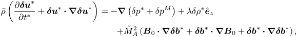 \begin{gather} \hskip-10pc\bar{\rho} \left( \frac{\partial \boldsymbol{\delta u}^*}{\partial t^*} + \boldsymbol{\delta u}^*\boldsymbol{\cdot} \boldsymbol{\nabla} \boldsymbol{\delta u}^* \right) ={-} \boldsymbol{\nabla} \left( \delta p^* + \delta p^M \right)+ \lambda \delta \rho^* \hat{\boldsymbol{e}}_z \nonumber\\ \hskip7pc\qquad + \tilde{M}_A^2 \left( \boldsymbol{B}_0 \boldsymbol{\cdot} \boldsymbol{\nabla} \boldsymbol{\delta b}^* + \boldsymbol{\delta b}^* \boldsymbol{\cdot} \boldsymbol{\nabla} \boldsymbol{B}_0 + \boldsymbol{\delta b}^* \boldsymbol{\cdot} \boldsymbol{\nabla} \boldsymbol{\delta b}^* \right), \end{gather}
 \begin{gather} \delta p^M = \tilde{M}_A^2 \left( \boldsymbol{B}_0 \boldsymbol{\cdot} \boldsymbol{\delta b}^* + \tfrac{1}{2} \left| \boldsymbol{\delta b}^* \right|^2 \right), \end{gather}
 \begin{gather} \frac{\partial \boldsymbol{\delta b}^*}{\partial t^*} + \boldsymbol{\delta u}^* \boldsymbol{\cdot} \boldsymbol{\nabla} \left( \boldsymbol{B}_0 + \boldsymbol{\delta b}^* \right) = \left( \boldsymbol{B}_0 + \boldsymbol{\delta b}^* \right) \boldsymbol{\cdot} \boldsymbol{\nabla} \boldsymbol{\delta u}^* - \left( \boldsymbol{B}_0 + \boldsymbol{\delta b}^* \right) \left( \boldsymbol{\nabla}\boldsymbol{\cdot} \boldsymbol{\delta u}^* \right), \end{gather}
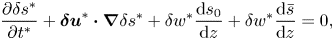 \begin{gather} \frac{\partial \delta s^*}{\partial t^*} + \boldsymbol{\delta u}^* \boldsymbol{\cdot} \boldsymbol{\nabla} \delta s^* + \delta w^* \frac{\mathrm{d} s_0}{\mathrm{d} z} + \delta w^* \frac{\mathrm{d} \bar{s}}{\mathrm{d} z}= 0, \end{gather}
 \begin{gather} \frac{\delta p^*}{\bar{p}} = \frac{\delta \rho^*}{\bar{\rho}} + \frac{\delta T^*}{\bar{T}}, \end{gather}
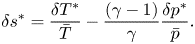 \begin{gather} \delta s^* = \frac{\delta T^*}{\bar{T}} - \frac{(\gamma - 1)}{\gamma} \frac{\delta p^*}{\bar{p}}. \end{gather}
The system (A1)–(A7) constitutes the standard equations of anelastic MHD, with  $\tilde {M}_A^2 = {O}(1)$ and $d/H_B = {O}(1)$.
A.2. Weak field-gradient anelastic equations
When the magnetic field is only weakly stratified, with  $\varepsilon _B \equiv d/H_B \ll 1$, the anelastic equations can be reduced further. To retain magnetic effects requires $\tilde {M}_A^2 = {O} (1/\varepsilon _B )$ (i.e. a stronger field than assumed in the standard anelastic approximation) and the following expansions:
 \begin{gather} \boldsymbol{B}_0 = \boldsymbol{B}_{00} + \varepsilon_B \boldsymbol{B}_{01} , \end{gather}
 \begin{gather}\boldsymbol{\delta b}^* = \varepsilon_B^{1/2} \boldsymbol{b}_\perp{+} \varepsilon_B \boldsymbol{b}_\parallel, \end{gather}
 \begin{gather}\boldsymbol{\delta u}^* = \boldsymbol{u}_\perp{+} \varepsilon_B^{1/2} \boldsymbol{u}_{{\parallel}}, \end{gather}
 \begin{gather}\boldsymbol{\nabla} = \boldsymbol{\nabla}_\perp{+} \varepsilon_B^{1/2} \boldsymbol{\nabla}_\parallel , \end{gather}
 \begin{gather}\delta p^M = \delta p_0^M + \varepsilon_B \delta p_1^M = \left( \boldsymbol{B}_{00} \boldsymbol{\cdot} \boldsymbol{b}_\parallel{+} \tfrac{1}{2} \left| \boldsymbol{b}_\perp \right|^2 \right) + \varepsilon_B \left( \boldsymbol{B}_{01} \boldsymbol{\cdot} \boldsymbol{b}_\parallel{+} \tfrac{1}{2} \left| \boldsymbol{b}_\parallel \right|^2 \right), \end{gather}
 \begin{gather}\frac{\mathrm{d} s_0}{\mathrm{d} z} = \beta_0^M + \varepsilon_B \beta_1^M = \left( \frac{\gamma-1}{\gamma} \frac{B_{00}}{\bar{p}} \frac{\mathrm{d} B_{01}}{\mathrm{d} z} \right) + \varepsilon_B\left( \frac{\gamma-1}{\gamma} \frac{B_{01}}{\bar{p}} \frac{\mathrm{d} B_{01}}{\mathrm{d} z} \right) . \end{gather}
Note that the  $\delta$-prefix has been dropped in (A9) and (A10) to ease notation. Substituting expansions (A8)–(A13) into (A1)–(A7) gives, at leading order, the following set of governing equations:
 \begin{gather} \boldsymbol{\nabla}_\perp \boldsymbol{\cdot} \left( \bar{\rho} \boldsymbol{u}_\perp \right) = 0, \end{gather}
 \begin{gather} \bar{\rho} \left( \frac{\partial }{\partial t^*} + \boldsymbol{u}_\perp \boldsymbol{\cdot} \boldsymbol{\nabla}_\perp \right) \boldsymbol{u}_\perp = {-} \boldsymbol{\nabla}_\perp \left( \delta p^* + \delta p_0^M \right) + \lambda \delta \rho^* {\hat{\boldsymbol{e}}}_z + \left( \boldsymbol{b}_\perp \boldsymbol{\cdot} \boldsymbol{\nabla}_\perp{+} \boldsymbol{B}_{00} \boldsymbol{\cdot} \boldsymbol{\nabla}_\parallel \right) \boldsymbol{b}_\perp, \end{gather}
 \begin{gather} \bar{\rho} \left( \frac{\partial }{\partial t^*} + \boldsymbol{u}_\perp \boldsymbol{\cdot} \boldsymbol{\nabla}_\perp \right) \boldsymbol{u}_\parallel={-} \boldsymbol{\nabla}_\parallel \left( \delta p^* + \delta p_0^M \right) + \left( \boldsymbol{b}_\perp \boldsymbol{\cdot} \boldsymbol{\nabla}_\perp{+} \boldsymbol{B}_{00} \boldsymbol{\cdot} \boldsymbol{\nabla}_\parallel \right) \boldsymbol{b}_\parallel{+} \boldsymbol{b}_\perp \boldsymbol{\cdot} \boldsymbol{\nabla}_\perp \boldsymbol{B}_{01} , \end{gather}
 \begin{gather} \frac{\partial \boldsymbol{b}_\perp}{\partial t^*} + \boldsymbol{u}_\perp \boldsymbol{\cdot} \boldsymbol{\nabla}_\perp \boldsymbol{b}_\perp{=} \left( \boldsymbol{b}_\perp \boldsymbol{\cdot} \boldsymbol{\nabla}_\perp{+} \boldsymbol{B}_{00} \boldsymbol{\cdot} \boldsymbol{\nabla}_\parallel \right) \boldsymbol{u}_\perp{-} \boldsymbol{b}_\perp \left( \boldsymbol{\nabla}_\perp \boldsymbol{\cdot} \boldsymbol{u}_\perp \right), \end{gather}
 \begin{gather} \frac{\partial \boldsymbol{b}_\parallel}{\partial t^*} + \boldsymbol{u}_\perp \boldsymbol{\cdot} \boldsymbol{\nabla}_\perp \left( \boldsymbol{B}_{01} + \boldsymbol{b}_\parallel \right) = \left( \boldsymbol{b}_\perp \boldsymbol{\cdot} \boldsymbol{\nabla}_\perp{+} \boldsymbol{B}_{00} \boldsymbol{\cdot} \boldsymbol{\nabla}_\parallel \right) \boldsymbol{u}_\parallel{-} \left( \boldsymbol{B}_{01} + \boldsymbol{b}_\parallel \right) \left( \boldsymbol{\nabla}_\perp \boldsymbol{\cdot} \boldsymbol{u}_\perp \right), \end{gather}
 \begin{gather} \boldsymbol{\nabla}_\perp \boldsymbol{\cdot} \boldsymbol{b}_\perp= 0, \end{gather}
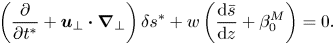 \begin{gather} \left( \frac{\partial }{\partial t^*} + \boldsymbol{u}_\perp \boldsymbol{\cdot} \boldsymbol{\nabla}_\perp \right) \delta s^* + w \left( \frac{\mathrm{d} \bar{s}}{\mathrm{d} z} + \beta_0^M \right)= 0. \end{gather}
Equations (A14)–(A20) constitute a new reduced sytem of equations, governing the weak field-gradient, strong field anelastic regime.
A.3. Boussinesq limits of anelastic equations
In this section we illustrate how to recover the Boussinesq magnetoconvection and magneto-Boussinesq equations by taking appropriate limits of the anelastic system. The Boussinesq equations are recovered in the limit of weak stratification, i.e.  $\lambda = d/H_p = \varepsilon _1 \ll 1$. The Boussinesq regime is characterised by typical flow speeds of ${O} ( (\varepsilon _1 \varepsilon _2 )^{1/2} c_s )$; such speeds are ${O} ( \varepsilon _1^{1/2} )$ slower than flow speeds in the anelastic regime. The typical dynamical time scale is thus correspondingly long: $(\varepsilon _1 \varepsilon _2)^{-1/2}$ times the acoustic time scale. Thus to recover the Boussinesq equations from the anelastic system, velocity and time need to be rescaled as
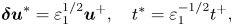 \begin{equation} \boldsymbol{\delta u}^* = \varepsilon_1^{1/2} \boldsymbol{u}^+ , \quad t^* = \varepsilon_1^{{-}1/2} t^+, \end{equation}
where we have used superscript ‘ $+$’ to denote further scaling of variables with a power of $\varepsilon _1$. We expand the thermodynamic variables – including both the reference state and perturbation – as follows:
 \begin{gather} \bar{\rho} = 1 + \varepsilon_1 \bar{\rho}_{1}, \quad \delta\rho^* = \delta\rho_0^* + \varepsilon_1 \delta\rho_1^*, \end{gather}
 \begin{gather}\bar{p} = 1 + \varepsilon_1 \bar{p}_{1}, \quad \delta p^* =\delta p_0^* + \varepsilon_1 \delta p_1^*, \end{gather}
 \begin{gather}\bar{T} = 1 + \varepsilon_1 \bar{T}_{1}, \quad \delta T^* = \delta T_0^* + \varepsilon_1 \delta T_1^*, \end{gather}
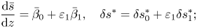 \begin{gather}\frac{\mathrm{d} \bar{s}}{\mathrm{d} z} = \bar{\beta}_0 + \varepsilon_1 \bar{\beta}_1,\quad \delta s^* = \delta s_0^* + \varepsilon_1 \delta s_1^*; \end{gather}
the quantity  $\bar {\beta }_0 \in \left \lbrace -1, +1 \right \rbrace$, where $\bar {\beta }_0 = -1 (+1)$ for a subadiabatic (superadiabatic) atmosphere. Depending on how we treat the magnetic field, we obtain either the equations of Boussinesq magnetoconvection or the magneto-Boussinesq equations.
A.3.1. Weak field-gradient magneto-Boussinesq equations
In comparison with the standard anelastic ordering, here the magnetic field stratification is weak (field gradient is  ${O}(\varepsilon _1)$) and the magnetic field strength accordingly stronger ( $\tilde {M}_A^2 = {O} (\varepsilon_1^{-1}$)). We therefore decompose the basic-state field as
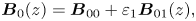 \begin{equation} \boldsymbol{B}_0(z)= \boldsymbol{B}_{00} + \varepsilon_1 \boldsymbol{B}_{01}(z) , \end{equation}
where  $\boldsymbol{B}_{00}$ is uniform. Magnetic fluctuations are ${O}(\varepsilon _1)$ smaller than the imposed field; thus we write
 \begin{equation} \boldsymbol{b}(\boldsymbol{ x }, t) = \varepsilon_1 \boldsymbol{b}_{1}. \end{equation}
The magnetic pressure fluctuation then becomes
 \begin{equation} \delta p^M =\delta p^M_{0} + \varepsilon_1 \delta p^M_{1} = \boldsymbol{b}_{1} \boldsymbol{\cdot} \boldsymbol{B}_{00} + \varepsilon_1 \left( \boldsymbol{b}_{1} \boldsymbol{\cdot} \boldsymbol{B}_{01} + \tfrac{1}{2}\left| \boldsymbol{b}_{1} \right|^2 \right) , \end{equation}
and the basic-state entropy gradient takes the form
 \begin{equation} \frac{\mathrm{d} s_0}{\mathrm{d} z} = \beta_0^M + {O}(\varepsilon_1) = \frac{(\gamma-1)}{\gamma} B_{00} \frac{\mathrm{d} B_{01}}{\mathrm{d} z} + {O}(\varepsilon_1) . \end{equation}
We express the fluctuation of total pressure  $\delta \varPi ^* = \delta p^* + \delta p^M$ as
 \begin{equation} \delta \varPi^* = \delta \varPi_0^* + \varepsilon_1 \delta \varPi_1^*, \end{equation}
the  $\boldsymbol{\nabla }$ operator as
 \begin{equation} \boldsymbol{\nabla} = \boldsymbol{\nabla}_\perp{+} \varepsilon_1 \boldsymbol{\nabla}_\parallel \end{equation}
and the fluid velocity as
 \begin{equation} \boldsymbol{u}^+= \boldsymbol{u}_{0}^+{+} \varepsilon_1 \boldsymbol{u}_{1}^+. \end{equation}
From the  ${O}(1)$ and ${O}(\varepsilon _1)$ terms in the anelastic continuity equation (A1), we obtain, respectively,
 \begin{gather} \boldsymbol{\nabla}_\perp \boldsymbol{\cdot} \boldsymbol{u}_{0}^+= 0, \end{gather}
 \begin{gather}\boldsymbol{\nabla}_\parallel \boldsymbol{\cdot} \boldsymbol{u}_{0}^+{+} \boldsymbol{\nabla}_\perp \boldsymbol{\cdot} \boldsymbol{u}_{1}^+{=} - w_{0}^+ \frac{\mathrm{d} \bar{\rho}_{1}}{\mathrm{d} z}. \end{gather}
As discussed in § 2, in the magneto-Boussinesq regime the total pressure variations  $\delta \varPi$ are ${O} ( \varepsilon _1 \varepsilon _2 )$; to satisfy this requirement we need $\delta \varPi _0^* = 0$ (recall $\delta \varPi = \varepsilon _2 \delta \varPi ^*$). Indeed, this is consistent with the ${O}(1)$ balance in the momentum equation, which reduces to $\boldsymbol{\nabla }_\perp \delta \varPi _0^* = 0$. It follows that the fluctuations in gas pressure and magnetic pressure cancel to leading order, i.e.
 \begin{equation} 0 = \delta p_0^* + \delta p_{0}^M. \end{equation}
Hence (negative) magnetic pressure replaces the thermodynamic pressure in the expressions for density and entropy perturbations (A6) and (A7),
 \begin{equation} \delta \rho_0^* ={-} \delta T_0^* - \delta p_{0}^M , \quad \delta s_0^* = {\delta T_0^*} + \frac{\gamma - 1}{\gamma} \delta p_{0}^M. \end{equation}
 At  ${O}(\varepsilon _1)$, the momentum equation (A2) becomes
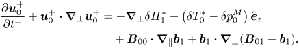 \begin{align} \frac{\partial \boldsymbol{u}_{0}^+}{\partial t^+} + \boldsymbol{u}_{0}^+ \boldsymbol{\cdot} \boldsymbol{\nabla}_\perp \boldsymbol{u}_{0}^+ &={-} \boldsymbol{\nabla}_\perp \delta \varPi_1^* - \left( \delta T_0^* - \delta p_{0}^M \right) {\hat{\boldsymbol{e}}}_z \nonumber\\ &\quad + \boldsymbol{B}_{00} \boldsymbol{\cdot} \boldsymbol{\nabla}_\parallel \boldsymbol{b}_{1} + \boldsymbol{b}_{1} \boldsymbol{\cdot} \boldsymbol{\nabla}_\perp (\boldsymbol{B}_{01} + \boldsymbol{b}_{1}) . \end{align}
At  ${O}(\varepsilon _1)$, the induction equation (A4), with use of (A34), gives
 \begin{equation} \left( \frac{\partial }{\partial t^+} + \boldsymbol{u}_{0}^+ \boldsymbol{\cdot} \boldsymbol{\nabla}_\perp \right) \left( \boldsymbol{B}_{01} + \boldsymbol{b}_{1} \right) = \left( \boldsymbol{B}_{00} \boldsymbol{\cdot} \boldsymbol{\nabla}_\parallel{+} \boldsymbol{b}_{1} \boldsymbol{\cdot} \boldsymbol{\nabla}_\perp \right)\boldsymbol{u}_{0}^+{+} w_{0}^+ \boldsymbol{B}_{00}\frac{\mathrm{d} \bar{\rho}_{1}}{\mathrm{d} z} . \end{equation}
The solenoidal constraint  $\boldsymbol{\nabla }\boldsymbol {\cdot } \boldsymbol{B} = 0$ reduces, at leading order, to
 \begin{equation} \boldsymbol{\nabla}_\perp{\cdot} \boldsymbol{b}_{1} = 0. \end{equation}
Finally, from the energy equation (A5), with use of (A36), we obtain the temperature equation
 \begin{equation} \left( \frac{\partial }{\partial t^+} + \boldsymbol{u}_{0}^+ \boldsymbol{\cdot} \boldsymbol{\nabla}_\perp \right) \left( \delta T_0^* + \frac{\gamma - 1}{\gamma} \delta p_{0}^M \right) + w_{0}^+ \left( \beta_0^M + \bar{\beta}_0 \right) = 0. \end{equation}
Equations (A33) and (A37)–(A40) constitute the governing equations for the description of magnetic buoyancy driven by a weak field gradient within the Boussinesq approximation, first derived by Spiegel & Weiss (Reference Spiegel and Weiss1982).
A.3.2. Strong field-gradient magneto-Boussinesq equations
Here, the field gradient is strong ( $d/H_B = {O} (1)$) and the field strength is such that $\tilde {M}_A^2 = {O}(1)$. We decompose the variables and gradient operator as
 \begin{gather} \boldsymbol{b}(\boldsymbol{ x }, t) = \boldsymbol{b}_\parallel{+} \varepsilon_1^{1/2} \boldsymbol{b}_\perp , \end{gather}
 \begin{gather}\delta p^M =\delta p^M_0 + \varepsilon_1 \delta p^M_1 = \tilde{M}_A^2 \left( \boldsymbol{B}_0\boldsymbol{\cdot} \boldsymbol{b}_\parallel{+} \tfrac{1}{2} \left| \boldsymbol{b}_\parallel \right|^2 \right) + \tfrac{1}{2}\varepsilon_1 \tilde{M}_A^2 \left| \boldsymbol{b}_\perp \right|^2 , \end{gather}
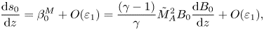 \begin{gather}\frac{\mathrm{d} s_0}{\mathrm{d} z} = \beta_0^M + {O}(\varepsilon_1) = \frac{(\gamma-1)}{\gamma} \tilde{M}_A^2 B_{0} \frac{\mathrm{d} B_{0}}{\mathrm{d} z} + {O}(\varepsilon_1), \end{gather}
 \begin{gather}\boldsymbol{u}^{+} = \boldsymbol{u}^{+}_\perp{+} \varepsilon_1^{{-}1/2} \boldsymbol{u}_{{\parallel}}^{+}, \end{gather}
 \begin{gather}\boldsymbol{\nabla} = \boldsymbol{\nabla}_\perp{+} \varepsilon_1^{1/2} \boldsymbol{\nabla}_\parallel. \end{gather}
Substituting expansions (A41)–(A45) into (A1)–(A7) and following similar arguments to those outlined in the weak gradient case above, we obtain the following set of magneto-Boussinesq equations:
 \begin{gather} \boldsymbol{\nabla}_\perp \boldsymbol{\cdot} \boldsymbol{u}_{{\perp}}^{+} + \boldsymbol{\nabla}_\parallel \boldsymbol{\cdot} \boldsymbol{u}_{{\parallel}}^{+} = 0, \end{gather}
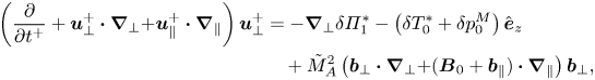 \begin{align} \left( \frac{\partial }{\partial t^{+}} + \boldsymbol{u}_\perp^{+} \boldsymbol{\cdot} \boldsymbol{\nabla}_\perp{+} \boldsymbol{u}_\parallel^{+} \boldsymbol{\cdot} \boldsymbol{\nabla}_\parallel \right)\boldsymbol{u}_\perp^{+} &={-}\boldsymbol{\nabla}_\perp \delta \varPi_1^* - \left( \delta T_0^* + \delta p_0^M \right) {\hat{\boldsymbol{e}}}_z \nonumber\\ &\quad + \tilde{M}_A^2 \left( \boldsymbol{b}_\perp \boldsymbol{\cdot} \boldsymbol{\nabla}_\perp{+} (\boldsymbol{B}_0 + \boldsymbol{b}_\parallel) \boldsymbol{\cdot} \boldsymbol{\nabla}_\parallel \right) \boldsymbol{b}_\perp , \end{align}
 \begin{gather} \left( \frac{\partial }{\partial t^{+}} + \boldsymbol{u}_\perp^{+} \boldsymbol{\cdot} \boldsymbol{\nabla}_\perp{+} \boldsymbol{u}_\parallel^{+} \boldsymbol{\cdot} \boldsymbol{\nabla}_\parallel \right)\boldsymbol{u}_\parallel^{+}= \tilde{M}_A^2 \left( \boldsymbol{b}_\perp \boldsymbol{\cdot} \boldsymbol{\nabla}_\perp{+} (\boldsymbol{B}_0 + \boldsymbol{b}_\parallel) \boldsymbol{\cdot} \boldsymbol{\nabla}_\parallel \right) \boldsymbol{b}_\parallel{+} \tilde{M}_A^2 \boldsymbol{b}_\perp \boldsymbol{\cdot} \boldsymbol{\nabla}_\perp \boldsymbol{B}_0, \end{gather}
 \begin{gather}\left( \frac{\partial }{\partial t^{+}} + \boldsymbol{u}_\perp^{+} \boldsymbol{\cdot} \boldsymbol{\nabla}_\perp{+} \boldsymbol{u}_\parallel^{+} \boldsymbol{\cdot} \boldsymbol{\nabla}_\parallel \right) \boldsymbol{b}_\perp{=} \left( \boldsymbol{b}_\perp \boldsymbol{\cdot} \boldsymbol{\nabla}_\perp{+} (\boldsymbol{B}_0 + \boldsymbol{b}_\parallel) \boldsymbol{\cdot} \boldsymbol{\nabla}_\parallel \right) \boldsymbol{u}_\perp^{+} , \end{gather}
 \begin{gather}\left( \frac{\partial }{\partial t^{+}} + \boldsymbol{u}_\perp^{+} \boldsymbol{\cdot} \boldsymbol{\nabla}_\perp{+} \boldsymbol{u}_\parallel^{+} \boldsymbol{\cdot} \boldsymbol{\nabla}_\parallel \right) \boldsymbol{b}_\parallel{+} \boldsymbol{u}_\perp^{+} \boldsymbol{\cdot} \boldsymbol{\nabla}_\perp \boldsymbol{B}_0 = \left( \boldsymbol{b}_\perp \boldsymbol{\cdot} \boldsymbol{\nabla}_\perp{+} (\boldsymbol{B}_0 + \boldsymbol{b}_\parallel) \boldsymbol{\cdot} \boldsymbol{\nabla}_\parallel \right) \boldsymbol{u}_\parallel^{+} , \end{gather}
 \begin{gather}\boldsymbol{\nabla}_\perp \boldsymbol{\cdot} \boldsymbol{b}_{{\perp}} + \boldsymbol{\nabla}_\parallel \boldsymbol{\cdot} \boldsymbol{b}_{{\parallel}} = 0, \end{gather}
 \begin{gather} \left( \frac{\partial }{\partial t^{+}} + \boldsymbol{u}_\perp^{+} \boldsymbol{\cdot} \boldsymbol{\nabla}_\perp{+} \boldsymbol{u}_\parallel^{+} \boldsymbol{\cdot} \boldsymbol{\nabla}_\parallel \right) \left( \delta T_0^* + \frac{\gamma - 1}{\gamma} \delta p_{0}^M \right) + w^+ \left( \beta_0^M + \bar{\beta}_0 \right) = 0, \end{gather}
where  $\delta p_0^M = \tilde {M}_A^2 \left ( {B}_0 {b}_\parallel + \frac {1}{2} {b}_\parallel ^2 \right )$, $\delta \varPi _1^* = \delta p_1^* +\frac {1}{2} \tilde {M}_A^2 {b}_\perp ^2$. Equations (A46)–(A52) constitute the governing equations for the description of magnetic buoyancy driven by a strong field gradient within the Boussinesq approximation, first derived by Bowker et al. (Reference Bowker, Hughes and Kersalé2014).
Note that a key difference between the (standard) weak field-gradient and strong field-gradient magneto-Boussinesq regimes is that, in the former, the velocity and magnetic field are solenoidal only in the plane perpendicular to the imposed field ((A33), (A39)), whereas in the latter the velocity and magnetic field are fully solenoidal ((A46), (A51)).
A.3.3. Boussinesq magnetoconvection equations
Here, the magnetic field is weaker than in the anelastic regime by a factor of  $\varepsilon _1^{1/2}$ (see table 1) and consequently $\tilde {M}_A^2 = {O} ( \varepsilon _1 )$. The momentum equation (2.23) at ${O} (1)$ gives $\boldsymbol{\nabla } p_0^* = 0$; hence $p_0^*$ is constant and can be set to zero without loss of generality. This is consistent with the ordering of pressure fluctuations as ${O}(\varepsilon _1 \varepsilon _2)$. As a result, pressure fluctuations do not enter the thermodynamics relations (A6) and (A7), and density and entropy fluctuations depend only on temperature variations:
 \begin{equation} \delta \rho_0^* ={-} \delta T_0^*, \quad \delta s_0^* = \delta T_0^*. \end{equation}
At leading order, the anelastic equations (A1)–(A5) reduce to those describing Boussinesq magnetoconvection (see, e.g. Chandrasekhar Reference Chandrasekhar1961; Weiss & Proctor Reference Weiss and Proctor2014):
 \begin{gather} \boldsymbol{\nabla}\boldsymbol{\cdot} \boldsymbol{u}^+= 0, \end{gather}
 \begin{gather}\left( \frac{\partial \boldsymbol{u}^+}{\partial t^+} + \boldsymbol{u}^+\boldsymbol{\cdot} \boldsymbol{\nabla} \boldsymbol{u}^+ \right) ={-} \boldsymbol{\nabla} \delta p_1^* - \delta T_0^* {\hat{\boldsymbol{e}}}_z + \left( \boldsymbol{\nabla}\times \boldsymbol{B}^* \right) \times \boldsymbol{B}^*, \end{gather}
 \begin{gather}\frac{\partial \boldsymbol{B}^*}{\partial t^+} + \left( \boldsymbol{u}^+ \boldsymbol{\cdot} \boldsymbol{\nabla} \right) \boldsymbol{B}^* = \left( \boldsymbol{B}^* \boldsymbol{\cdot} \boldsymbol{\nabla} \right) \boldsymbol{u}^+, \end{gather}
 \begin{gather}\left( \frac{\partial }{\partial t^+} + \boldsymbol{u}^+\boldsymbol{\cdot} \boldsymbol{\nabla} \right) \delta T_0^* + \bar{\beta}_0 w^+= 0. \end{gather}


 Open access