1. Introduction
How is the Big Bang’s correctness investigated?! Big Bang is based on three pillars: the Cosmic Microwave Background Radiation (CMBR or CMB), the universe inflation, and the Big Bang Nucleosynthesis (BBN), the first two of which have been proved both theoretically and experimentally. However, the third one has been faced with a serious problem. As one of the main branches of the nucleosynthesis theory in nuclear astrophysics, through studying the universe evolution using nuclear reactions, the BBN seeks to calculate the rates of the primary reactions of the very first moments of the Big Bang. Based on this theory, the Big Bang leads to the production of hydrogen (and its isotopes including deuterium and tritium), helium, and a little lithium through primary reactions network during the first 3 minutes of the universe life (Cowan et al. Reference Cowan and Thielemann2004; Coc Reference Coc2016; Weinberg Reference Weinberg1993). In this regard, the calculated values for the abundances of produced hydrogen, deuterium, and helium are in perfect agreement with the experimental measured values of the astrophysical observations. But the calculated value for the lithium abundance is three times (Iliadis et al. Reference Iliadis and Coc2020) the experimentally measured value. This discrepancy is known as the cosmological Lithium problem in BBN. The explanations for the lithium problem include unknown systematic effects in 7Li observations, possible errors in thermonuclear reaction rates affecting the lithium and beryllium synthesis, physics beyond the standard model, and imprecise awareness of lithium developments in stars, despite the determined possible locations for each nuclei (Iliadis Reference Iliadis2023).
However, it is believed that solving process of the lithium problem from the point of view of nuclear physics depends on the accurate calculation of the nucleosynthesis reaction rates related to the production or destruction of lithium and determining their exact abundances. Therefore, if the mentioned discrepancy is solved, the correctness of the BBN and then the Big Bang theory can be proved.
In this regard, many researches have been already focused on this problem and this field of research to calculate the exact value of reaction rates, such as Descouvemont et al. (Reference Descouvemont, Adahchour, Angulo, Coc and Vangioni-Flam2004) and Coc et al. (Reference Coc, Petitjean, Uzan, Vangioni, Descouvemont, Iliadis and Longland2015) using R-matrix and χ2-minimisation fits and Adelberger et al. (Reference Adelberger2011) for solar system. But lack of enough experimental data for some important reactions forces the researchers to use other methods compatible with the harsh situation of the lack of data that limits the possibility of accurate calculations. The new methods include Bayesian statistics that fits the mentioned harsh situation and will be explained in Section 3.
Therefore, in order to improve the mentioned discrepancy through exact calculating the S-factor and the reaction rates, this study investigates the S-factor and the reaction rate of T(d,n)4He as a part of the BBN reactions network using a new method, and for this purpose, Bayes’ principle and nuclear R-matrix theory are simultaneously used to infer an accurate output using available limited experimental data.
2. Importance of the T(d,n)4He reaction
Before this study, a number of studies had focused on the calculation of the rates of some reactions of the BBN reaction network (Fig. 1) using Bayesian method, such as d(p,γ)3He, 3He(3He,2p)4He and 3He(α,γ)7Be (Iliadis et al. Reference Iliadis, Anderson, Coc, Timmes and Starrfield2016), d(d,n)3He and d(d,p)3H (Iñesta, Iliadis, & Coc Reference Iñesta, Iliadis and Coc2017), 3He(d,p)4He (de Souza et al. Reference De Souza, Boston, Coc and Iliadis2019a), 7Be(n,p)7Li (de Souza et al. Reference De Souza, Kiat, Coc and Iliadis2020), 3H(d,n)4He (De Souza, Iliadis, & Coc Reference De Souza, Iliadis and Coc2019b), d(p,γ)3He (Moscoso et al. Reference Moscoso, De Souza, Coc and Iliadis2021), and 16O(p,γ)17F (Iliadis, Palanivelrajan, & de Souza Reference Iliadis, Palanivelrajan and de Souza2022), all of which have been reviewed by (Esmaeili et al. Reference Esmaeili, Ghasemizad, Naserghodsi and Sendesi2022).
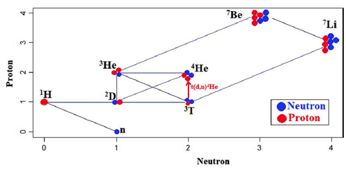
Figure 1. Big Bang Nucleosynthesis reaction network according to Nakamura et al. (Reference Nakamura, Hashimoto, Ichimasa and Arai2017). Each line represents a nuclear reaction.
Among the BBN reactions network, the T(d,n)4He reaction has been selected for this study, which has been marked with a red colour in Fig. 1.
The T(d,n)4He reaction is considered as one of the most important reactions of the nuclear fusion for future terrestrial nuclear reactors because of its theoretical high nuclear gain of about 450–1 000. It is even considered and investigated as a space propulsion source or a power source (Chapman Reference Chapman2011) and also as a source of energy production in stars, which has the highest cross section and the amount of energy produced per reaction, which leads to the stable nucleus of 4He, and is also the basis of higher stages of fusion in older stars, hence one of the affecting factors on the lithium problem in BBN. This reaction is also considered as a possible source of intermediate energy ranged neutrons (Gagliardi et al. 1989) that can be used in different laboratories.
Because of its importance, as mentioned earlier, this reaction has been investigated by de Souza et al. (Reference De Souza, Iliadis and Coc2019b), which resulted in better and improved S-factor and reaction rate, having lower calculation uncertainties. For the same reasons, this study tries to do the same investigation but with some different considerations in its performed method, which is described in the next section.
3. Method
In this study, Bayesian statistics is used as a new statistical method for nuclear calculations on the basis of limited available data, because it gives results with lower uncertainties in comparison with non-Bayesian methods (such as methods on the basis of χ2-minimisation). Bayes’ principle (or Bayesian statistics) is used to fit the existing experimental data in order to further extrapolations. Bayes’ principle in one of its applied forms can be expressed as follows:
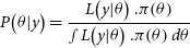 \begin{align}P\!\left( {\theta {\rm{|}}y} \right) = \frac{{L\!\left( {y{\rm{|}}\theta } \right).\pi \!\left( \theta \right)}}{{\smallint L\!\left( {y{\rm{|}}\theta } \right).\pi \!\left( \theta \right)d\theta}}\end{align}
in which, the numerator expresses the product of the likelihood [ $L\!\left( {y{\rm{|}}\theta } \right)$
] (a postulated nuclear model) and the probability density of the priors [π(θ)] (primary form of the studied parameters in term of distribution functions), which gives the posterior
$L\!\left( {y{\rm{|}}\theta } \right)$
] (a postulated nuclear model) and the probability density of the priors [π(θ)] (primary form of the studied parameters in term of distribution functions), which gives the posterior $\left[ {P\!\left( {\theta {\rm{|}}y} \right)} \right]$
(the updated distribution functions of the parameters as the output of the study) (de Souza et al. Reference De Souza, Kiat, Coc and Iliadis2020). The denominator of the Equation (1) is a normalisation factor that has no special role in the calculations of this study and is considered as one, because the summation of all the possible probabilities is one. The likelihood in most of nuclear astrophysical calculations is defined as a product of the used distribution function for the astrophysical S-factor and the statistical uncertainty. This form of statistics uses a very scant experimental data of a phenomenon in order to estimate the best treat for that phenomenon.
$\left[ {P\!\left( {\theta {\rm{|}}y} \right)} \right]$
(the updated distribution functions of the parameters as the output of the study) (de Souza et al. Reference De Souza, Kiat, Coc and Iliadis2020). The denominator of the Equation (1) is a normalisation factor that has no special role in the calculations of this study and is considered as one, because the summation of all the possible probabilities is one. The likelihood in most of nuclear astrophysical calculations is defined as a product of the used distribution function for the astrophysical S-factor and the statistical uncertainty. This form of statistics uses a very scant experimental data of a phenomenon in order to estimate the best treat for that phenomenon.
All the basic considered parameters of the used model (likelihood) in this study are based on the nuclear R-matrix theory. According to previous studies in this field, the S-factor, as an astrophysical replacement for nuclear cross section, in single-level two-channel R-matrix theory can be written as:
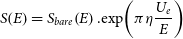 \begin{align}S\!\left( E \right) = {S_{bare}}\!\left( E \right).{\rm{exp}}\!\left( {\pi \eta \frac{{{U_e}}}{E}} \right)\end{align}
 \begin{align}2\pi \eta = 0.98951013{Z_0}{Z_1}\sqrt {\frac{{{M_0}{M_1}}}{{{M_0} + {M_1}}}\frac{1}{E}} \end{align}
where S bare is for a nucleus without electron screening effect, 2πη is the Sommerfeld parameter, and U e is the electron screening potential (Iliadis Reference Iliadis2015). Based on Baye et al. (Reference Baye and Brainis2000), one can approximate and expand the S-factor parameter using Taylor series (expansion) as follows:
 \begin{align}{S_{bare}}\!\left( E \right) = S\!\left( 0 \right) + S'\!\left( 0 \right)E + \frac{1}{2}S''\!\left( 0 \right){E^2}\end{align}
in which, to calculate the S bare using R-matrix theory, the following nuclear relation is considered:
 \begin{align}{S_{bare}}\!\left( E \right) = E.\exp\!\left( {2\pi \eta } \right).{\sigma _{dn}}\!\left( E \right)\end{align}
in which, the reaction cross section ( ${\sigma _{dn}}$
) is
${\sigma _{dn}}$
) is
 \begin{align}{\sigma _{dn}}\!\left( E \right) = \frac{\pi }{{k_d^2}}\frac{{2J + 1}}{{\left( {2{J_1} + 1} \right)\left( {2{J_2} + 1} \right)}}{\left| {{S_{dn}}} \right|^2}\end{align}
where k d is the deuteron (projectile) wave number, J 1=1/2 and J 2=1 are the spins of the T (or 3H) and deuteron ground state, respectively, with (J=3/2) in this study, and S dn is the scattering matrix element as follows:
 \begin{align}{\left| {{S_{dn}}} \right|^2} = \frac{{{{\rm{\Gamma }}_d}{{\rm{\Gamma }}_n}}}{{{{\left( {{E_0} + {\rm{\Delta }} - {E_r}} \right)}^2} + {{\left( {{\rm{\Gamma }}/2} \right)}^2}}}\end{align}
where Γ d and Γ n are, respectively, the partial widths of the input channel 3H + d and the output channel 4He + n, Γ is the total width, Δ is the level shift, E 0 is eigenvalue of energy, and E r is the resonance energy of the studied reaction. The partial and total widths, and the level shift follow the below equations, respectively:
 \begin{align}{\rm{\Gamma }} = \mathop \sum \limits_c {{\rm{\Gamma }}_c},\;\;{{\rm{\Gamma }}_c} = 2\gamma _c^2{{\rm{P}}_c}\end{align}
where γ2 c is the reduced width, B c is the boundary condition parameter, and the energy-dependent quantities P c and S c are, respectively, the penetration factor and shift factor for channel c of a reaction (each of the two allowed reaction channels in this study) as:
 \begin{align}{{\rm{P}}_c} &= \frac{{{{\rm{k}}_d}{{\rm{a}}_c}}}{{F_\ell ^2 + G_\ell ^2}},\;\;\nonumber \\[5pt] {{\rm{S}}_c} &= \frac{{{{\rm{k}}_d}{{\rm{a}}_c}\!\left( {F_\ell ^{}\;\,F_\ell ^{\prime} + G_\ell ^{}\;\, G_\ell ^{\prime}} \right)}}{{F_\ell ^2 + G_\ell ^2}}\end{align}
in which ℓ is the orbital angular momentum of the reaction channel. The other useful parameter in R-matrix theory is a c as the radius of the reaction channel:
 \begin{align}{{\rm{a}}_c} = {{\rm{r}}_0}\!\left( {A_1^{\frac{1}{3}} + A_2^{\frac{1}{3}}} \right)\end{align}
where A 1 and A 2 are the mass numbers of two interacting nuclei (here, T and D), and r 0 is a constant number between 1 and 2 fm.
The above-mentioned parameters are introduced in the Bayesian model of this study as the fitting parameters in the forms of probability density functions (PDF), which finally will result in the extrapolated S-factor distribution.
At the end, by numerical integration of reaction rate Equation (12), using the resulted S-factor, the reaction rates of T(d,n)4He are calculated for temperatures in the range of 1 MK to 10 GK:
 \begin{align}{N_A}\sigma \upsilon = {\left( {\frac{8}{{\pi {m_{01}}}}} \right)^{\frac{1}{2}}}\frac{{{N_A}}}{{{{\left( {kT} \right)}^{\frac{3}{2}}}}} \mathop {}^{\ast}\smallint \nolimits_0^\infty S\!\left( E \right).\exp\!\left( { - 2\pi \eta } \right)\exp\!\left( { - \frac{E}{{kT}}} \right)dE\end{align}
where m 01 is the reduced mass of the target and projectile, and kT is in term of MeV, which corresponds to Giga Kelvin temperatures.
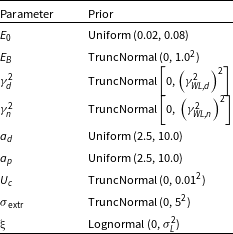
However, the defined model in R-software for Bayesian analysis includes two types of parameters: physical parameters (resonance energy, reduced widths, and channel radii) and experimental parameters (data uncertainty and normalisation coefficients). Of course, in the end, only the S-factor is reported as the final goal of this study. Same as de Souza et al. (Reference De Souza, Kiat, Coc and Iliadis2020), in this study, the defined normal probability densities related to the priors of the physical parameters are truncated at zero (to not being negative). The considered priors are specified in Table 1 ( $\gamma _{WL}^2 \approx \frac{\hbar }{{\mu .{a^2}}}$
is the Wigner limit with reduced mass
$\gamma _{WL}^2 \approx \frac{\hbar }{{\mu .{a^2}}}$
is the Wigner limit with reduced mass $\mu $
of the interacting components, Bohr radius
$\mu $
of the interacting components, Bohr radius $a$
, and Planck constant
$a$
, and Planck constant $\hbar $
).
$\hbar $
).
Table 1. The priors of the Bayesian model of this study.
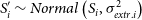
The calculating Markov chain of this study is based on a Metropolis–Hastings algorithm, and the model used to calculate the S-factor has the following nested form that contrary to de Souza et al. (Reference De Souza, Iliadis and Coc2019b) and has four chains with the length of 50 000 and Burn-in of 1 000:
 \begin{align}S_i^{\prime}\sim Normal\left( {{S_i},\sigma _{extr.i}^2} \right)\end{align}
 \begin{align}S_{i,j}^{\prime\prime} = {f_{S,j}} \times S_i^{\prime}\end{align}
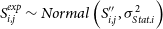 \begin{align}S_{i,j}^{exp}\sim Normal\left( {S_{i,j}^{\prime\prime},\sigma _{Stat.i}^2} \right)\end{align}
where S i is the experimental data of the S-factor, f s is the statistical scaling factor, and σ represents the mentioned uncertainties of the calculations. For the scaling factor (f s ), which is a number close to 1, the non-informative prior function was introduced with the form of the normal PDF, which has a mean value of 0 and a standard deviation of 100, and was again truncated at 0 to be positive. The indices ‘extr’ stand for the total unknown sources of the uncertainties, including statistical uncertainty and systematic uncertainty.
Furthermore, the experimental data points that were used as the input data into the defined model, along with the results of the defined model of this study for data extrapolation, will be mentioned later in the next section.
4. Results and discussion
At first, it must be mentioned that, since all experiments are faced with uncertainties, which are divided into two Statistical and Systematic uncertainties, we have a reaction rate or equivalently the astrophysical S-factor as $S_{ \pm sys}^{ \pm stat}$
, with
$S_{ \pm sys}^{ \pm stat}$
, with $ \pm stat$
and
$ \pm stat$
and $ \pm sys$
showing the statistical and systematic uncertainties, respectively.
$ \pm sys$
showing the statistical and systematic uncertainties, respectively.
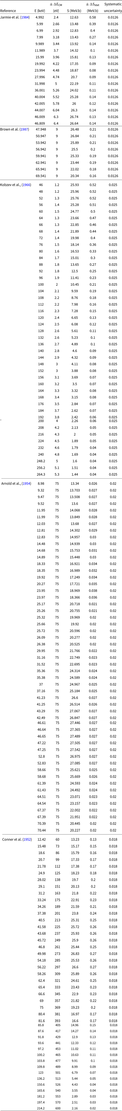
There are a few data for S-factor in some limited areas of energy. In this study, all of the available datasets for the reaction are simultaneously used to find the curve of the studied quantity and also to estimate the value of S-factor in the missed areas using statistical fitting methods, such as extrapolations that are based on Bayesian principal. It must be emphasised that the mentioned data points are all of the available valid data that are based on experiments. However, to analyse the behaviour of the astrophysical S-factor (equivalent to the cross section) of the deuterium-tritium reaction, T(d,n)4He, in the low-energy regions, the data of Jarmie et al. (Reference Jarmie, Brown and Hardekopf1984), Brown, Jarmie, & Hale (Reference Brown, Jarmie and Hale1987), Kobzev et al. (Reference Kobzev, Salatskij and Telezhnikov1966), Arnold et al. (Reference Arnold, Phillips and Sawyer1954), and Conner, Bonner, & Smith (Reference Conner, Bonner and Smith1952) (see Appendix A) were used in our Bayesian model mentioned in Section 3, which resulted in Fig. 2 as the data fit for the astrophysical S-factor.
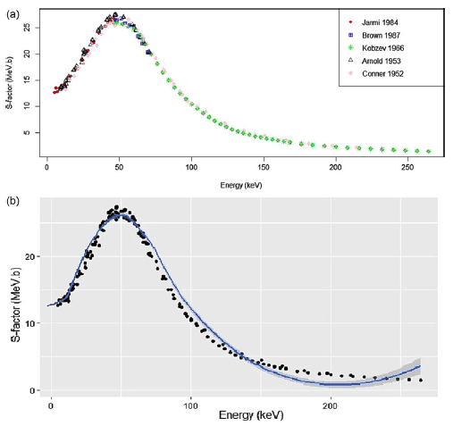
Figure 2. The astrophysical S-factor (equivalent to the cross section) for T(d,n)4He. Panel (a) shows the distribution of the data points, and the panel (b) shows the Bayesian fit for the data points as a blue line, and the grey credible interval.
As can be seen, the behaviour of the S-factor at low energies is dominated by a broad resonance at an energy lower than 50 keV, and as the energy decreases, its value also drops to about 12 MeV.b.
However, after the final fitting process, the value of ${S_{bare - 0}} = 12.11_{ \pm 0.091}^{ \pm 0.089}\;{\rm{MeV}}.{\rm{b}}$
was obtained that found to be in very good agreement with the results of de Souza et al. (Reference De Souza, Iliadis and Coc2019b) in their Fig. 3, with a very slight difference: the uncertainty value in this study is slightly higher than those of de Souza et al. (Reference De Souza, Iliadis and Coc2019b). Also, in comparison, for example, with
${S_{bare - 0}} = 12.11_{ \pm 0.091}^{ \pm 0.089}\;{\rm{MeV}}.{\rm{b}}$
was obtained that found to be in very good agreement with the results of de Souza et al. (Reference De Souza, Iliadis and Coc2019b) in their Fig. 3, with a very slight difference: the uncertainty value in this study is slightly higher than those of de Souza et al. (Reference De Souza, Iliadis and Coc2019b). Also, in comparison, for example, with ${{\rm{S}}_{0.04}} = 25.87 \pm 0.49\;{\rm{MeV}}.{\rm{b}}$
from Bosch et al. (Reference Bosch and Hale1992), which obviously represents higher uncertainties, the results of the Bayesian method yields lower uncertainties, hence a better result. It should be noted that the value reported by de Souza et al. (Reference De Souza, Iliadis and Coc2019b) for the S-factor is not for zero energy (
${{\rm{S}}_{0.04}} = 25.87 \pm 0.49\;{\rm{MeV}}.{\rm{b}}$
from Bosch et al. (Reference Bosch and Hale1992), which obviously represents higher uncertainties, the results of the Bayesian method yields lower uncertainties, hence a better result. It should be noted that the value reported by de Souza et al. (Reference De Souza, Iliadis and Coc2019b) for the S-factor is not for zero energy ( $ \ne $
S0), but instead, for the value of S-factor in energies about 0.04 (
$ \ne $
S0), but instead, for the value of S-factor in energies about 0.04 ( ${S_{0.04}} = 25.438_{ \pm 0.089}^{ \pm 0.080}\;{\rm{MeV}}.{\rm{b}}$
), which is again in very close agreement with the value obtained in the diagram of Fig. 2 of this study. Regarding this difference between the reported S-factors for different energy regions, the reported S-factors of the two studies just apparently seem to be different, but in fact, they are not, since the S-factor on the 0.04 MeV in this study is
${S_{0.04}} = 25.438_{ \pm 0.089}^{ \pm 0.080}\;{\rm{MeV}}.{\rm{b}}$
), which is again in very close agreement with the value obtained in the diagram of Fig. 2 of this study. Regarding this difference between the reported S-factors for different energy regions, the reported S-factors of the two studies just apparently seem to be different, but in fact, they are not, since the S-factor on the 0.04 MeV in this study is ${S_{0.04}} = 25.518_{ \pm 0.088}^{ \pm 0.085}\;{\rm{MeV}}.{\rm{b}}$
, which is closely similar to the one reported by de Souza et al. (Reference De Souza, Iliadis and Coc2019b) at the same energy.
${S_{0.04}} = 25.518_{ \pm 0.088}^{ \pm 0.085}\;{\rm{MeV}}.{\rm{b}}$
, which is closely similar to the one reported by de Souza et al. (Reference De Souza, Iliadis and Coc2019b) at the same energy.
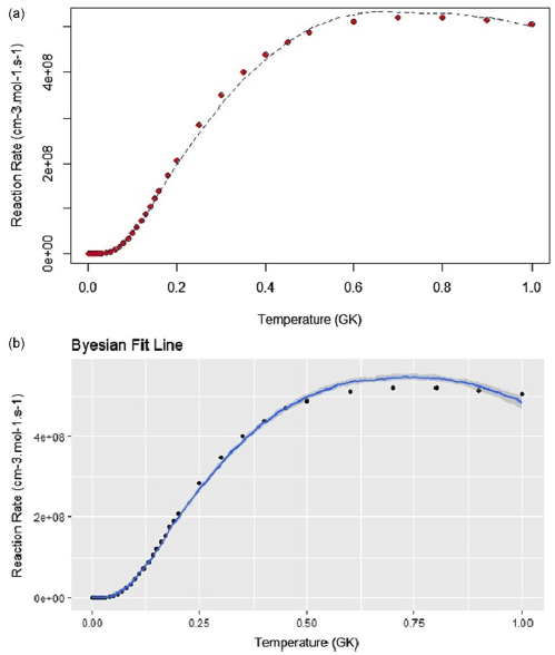
Figure 3. Reaction rate at GK for T(d,n)4He. Panel (a) shows the distribution of the reaction rate data points, and the panel (b) shows the Bayesian fit for them as a blue line, and the grey credible interval.
Furthermore, for the electron screening effect, as can be seen in Fig. 2 as the astrophysical S-factor variation diagram, at very low energies (less than 10 keV), no significant electron screening effect can be expressed for this reaction, and only a limit can be considered, which of course will have a small value (about only a few eV), and for this reason, the S-factor diagram does not increase at very low energies under the influence of this effect and does not goes up but instead is stopped at a certain value. The result of this study as the non-significant electron screening effect for the T(d,n)4He reaction is in full agreement with the result of de Souza et al. (Reference De Souza, Iliadis and Coc2019b), while this result disagree with the reports of some studies, including Langanke et al. (Reference Langanke and Rolfs1989). The agreement between the results of this study and those of de Souza et al. (Reference De Souza, Iliadis and Coc2019b) shows that choosing a higher number of Markov chains with different length and Burn-in does not make significant differences on the final results.
Moreover, from the diagram of Fig. 2, it can be seen that the data of Kobzev et al (Reference Kobzev, Salatskij and Telezhnikov1966) in the sequence of higher energies describes the behaviour of the S-factor better than those of Kobzev et al. (Reference Kobzev, Salatskij and Telezhnikov1966) and also Arnold et al. (Reference Arnold, Phillips and Sawyer1954), whose data provide a better description of the S-factor in low energies, while the study of Conner et al. (Reference Conner, Bonner and Smith1952) describes the variations of the S-factor very well in both high- and low-energy regions.
At the end, using the resulted S-factor (S bare ), and after replacing it in the reaction rate formula (Equation (12)), the reaction rate values can be calculated for a range of temperatures, whose output graph is as Fig. 3 indicates.
The reaction rate curve has been plotted by numerical integration of Equation (12) using the same S-factor (S-bare) of the previous section (calculated using the Bayesian model) and considering the 50th percentiles of the deduced probability densities. These values can be found in Appendix B.
It can be seen in Fig. 3 that with the increase in the temperature, since the kinetic energy of the interacting particles increases, conditioned by enough or high abundances of deuteron and tritium in the environment, the reaction rate grows until it reaches a limit of about $5 \times {10^8}\;{\rm{c}}{{\rm{m}}^{ - 3}}{\rm{mo}}{{\rm{l}}^{ - 1}}{{\rm{s}}^{ - 1}}$
. Of course, further growth of the reaction rate is possible and is not limited to the mentioned value, but the conditions and temperature of the environment (the energy of the interacting particles) play vital roles in the occurrence of the reaction. At the lower temperatures (energies), due to the energy decrease of the interacting particles (deuterium and tritium), which are less able to penetrate the Coulomb repulsive barrier, the reaction rate undergoes a sharp exponential decrease and gives a value close to zero, which can be seen in the diagram, but this reduction of the rate to zero is actually due to the insignificant rate of the reaction, and in practice, it does not exactly mean as the complete cessation of the reaction in the star environment.
$5 \times {10^8}\;{\rm{c}}{{\rm{m}}^{ - 3}}{\rm{mo}}{{\rm{l}}^{ - 1}}{{\rm{s}}^{ - 1}}$
. Of course, further growth of the reaction rate is possible and is not limited to the mentioned value, but the conditions and temperature of the environment (the energy of the interacting particles) play vital roles in the occurrence of the reaction. At the lower temperatures (energies), due to the energy decrease of the interacting particles (deuterium and tritium), which are less able to penetrate the Coulomb repulsive barrier, the reaction rate undergoes a sharp exponential decrease and gives a value close to zero, which can be seen in the diagram, but this reduction of the rate to zero is actually due to the insignificant rate of the reaction, and in practice, it does not exactly mean as the complete cessation of the reaction in the star environment.
The exponential curve of Fig. 3 is an estimate of the likely behaviour of the reaction rate function with respect to temperature. As mentioned, the changes of the reaction rate of T(d,n)4He can be considered as relatively exponential.
Reconsidering the changes of the temperature, the energy and the resulted astrophysical S-factor for the d-t reaction in terms of each other obtains the following contour plots of Figs. 4 and 5.
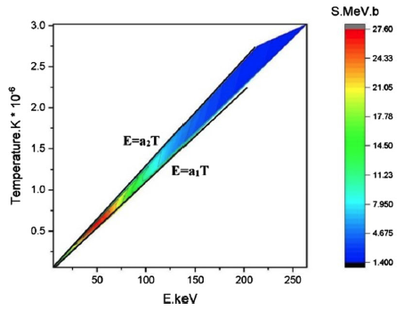
Figure 4. Astrophysical S-factor (MeV.b) contour plot as a quantity for reaction rate in terms of temperature (Kelvin) and energy (keV) for the T(d,n)4He reaction.

Figure 5. Astrophysical S-factor (MeV.b) contour plot as a quantity for reaction rate in terms of logarithmic temperature (Kelvin) and energy (keV) for the T(d,n)4He reaction.
In the graph of Fig. 4, the blue area shows the lowest S-factors, while the red area shows the highest values of the S-factor in terms of temperature and energy. As can be seen in the contour plot of Fig. 4, the value of the S-factor at an energy of about 50 keV and a temperature of about 5.8 K has a maximum value, which is actually the resonance of the cross section of the reaction in the mentioned energy (temperature) region. But in the areas around it, the S-factor decreases, which is a good representation of the resonant behaviour of the cross section of the studied reaction in this energy range; hence a proof that the studied reaction has a resonant behaviour in this region.
Also, the presence of S-factor values can be seen only in the upper regions of above the line E=a 1 T. It should be noted that the energy and temperature of the stellar environment, where the reactions take place, are actually equivalent concepts in nuclear physics, hence linearly dependent on each other with a coefficient as a 1 . As a result, the linear dependence of these two quantities can be seen as black diagonal lines having the slope of a 1 and a 2 . Naturally, in the area below the line E=a 1 T, the S-factor does not have any values, because in this area, temperature and energy are not of the same nature; hence, a specific cross section cannot be obtained in this circumstance. The slope a 1 indicating the dependence between the two quantities of energy and temperature as E=a 1 T is the conversion coefficient between two mentioned quantities in nuclear physics (a 1=11 600 eV/300 K = 38.67 eV K-1).
It is also noteworthy that the value of the S-factor will be limited to a certain upper limit. Therefore, according to the diagram, the value of S-factor will be between the two border regions of E=a 1 T and E=a 2 T. The slope of the upper boundary line (a2) will depend on the value of different values of the S-factor, because especially for some energy and temperature values, several close cross sections (S-factor) are obtained from different studies. As a result, the resulting contour plot will have two boundaries (or a hill-top point in its 3D view).
In the diagram of Fig. 5, where the temperature has been plotted logarithmically, again the S-factor is maximised in the energy of about 50 keV and the logarithmic temperature equal to about 0.58 (with the corresponding unit), showing the same resonance that was mentioned before, and having the same dependence line of energy and temperature as E=a 1 T(a 1=11 600 eV/300 K = 38.67 eV K−1).
The importance of the two diagrams of Figs. 4 and 5 is that the simultaneous dependence of the astrophysical S-factor on both energy and temperature quantities can be seen, and at the same time, the resonance in the cross section of the reaction is well evident.
However, as a comparison with this study, the model used by de Souza et al. (Reference De Souza, Iliadis and Coc2019b) had three longer chains, while the model of this study uses four shorter chains instead, to investigate the calculation independency of the number and length of the chains. It must be mentioned that the whole other studies in this field, such as Iliadis et al. (Reference Iliadis, Anderson, Coc, Timmes and Starrfield2016), de Souza et al. (Reference De Souza, Boston, Coc and Iliadis2019a), (Reference De Souza, Kiat, Coc and Iliadis2020), Moscoso et al. (Reference Moscoso, De Souza, Coc and Iliadis2021), and Iliadis et al. (Reference Iliadis, Palanivelrajan and de Souza2022) have used three chains for their calculations.
Furthermore, this study mainly uses dnorm and dunif functions for its defined models so as to consider a normal distributions for the input data, which makes no significant difference on the final results in comparison with other studies, such as de Souza et al. (Reference De Souza, Iliadis and Coc2019b).
However, according to the numerical values obtained for the studied reaction (increase in the cross section and as a result, the increase in the reaction rate of T(d,n)4H), and by referring to Fig. 1, it can be seen that this increase will require more deuteron consumption; therefore, the amount of the conversion of these two nuclei into lithium will reduce to a negligible extent, which confirms the reduction of the discrepancy between the theoretical and experimental values of lithium abundances, hence leading to an improvement in lithium problem. But due to the slight decrease of this value, it cannot be claimed that the existing problem has been completely resolved, but only an insignificant reduction (in the range of only a few percent compared to the difference of three times between the theoretical and experimental values) will be resulted, and the lithium problem will still remain, the reason for which should be in other cases, including a correction on the Big Bang theory.
5. Conclusion
In this study, using the R-program (R Core team 2015), four short Markov chains using a Bayesian model (likelihood) having different components with different values and distribution functions in comparison with latest studies in this field were used in order to find the behaviour of the astrophysical S-factor and consequently the reaction rate for T(d,n)4He as one of the most important reactions in nuclear astrophysics, playing a crucial role in BBN.
As the first result, making changes in the defined models and functions with different imported values and also changing the Markov chains made no significant difference in the final values of the S-factor or the studied reaction rate.
Also, as the second result of this study, despite the innovation and efficiency of Bayesian method, only little improvements have been made on the primary lithium abundances. Therefore, to justify this condition and the inadequacy of the models used so far to solve the lithium problem, this interpretation can be proposed that these kinds of calculations have no significant impact on the abundance of lithium, and as a result, the reason for the discrepancy between the theoretical and experimental values of the initial abundance of lithium should be explained using other considerations, including a new correct knowledge of the lithium destruction mechanism in proto-stars or the need for a new related physics theory, especially correcting the Big Bang theory in some of its aspects, such as BBN development process, star evolution process, or so on.
Therefore, despite the correctness and effectiveness of the current calculations, the need to complete such calculations is still remained and other factors should and can be included in to fully solve the lithium problem.
Competing interest
The authors declare that they have no known competing financial interests or personal relationships that could have appeared to influence the work reported in this paper.
Data Availability
Not applicable.
Appendix A. The data used for the T(d,n)4He reaction calculations