


INTRODUCTION AND BACKGROUND
The Greenland ice sheet (GrIS) mass loss and its contribution to sea-level rise has more than quadrupled from 1991–2001 to 2002–11 (Shepherd and others, Reference Shepherd2012) due to both increased discharge of ice to the ocean and decreased surface mass balance (Van den Broeke and others, Reference Van den Broeke2009, Reference Van den Broeke2016; Enderlin and others, Reference Enderlin2014; Velicogna and others, Reference Velicogna, Sutterley and Van Den Broeke2014; Khan and others, Reference Khan2014). The partitioning of mass loss between dynamic (i.e. changes in ice flow, thinning and calving rates) and surface processes is important because these losses indicate different forcing (Howat and others, Reference Howat2011). While surface mass balance is driven by atmospheric processes, tidewater glacier dynamics are driven by changes in resistive stress at the terminus (e.g. Nick and others, Reference Nick, Vieli, Howat and Joughin2009), likely triggered by changing ocean conditions (Holland and others, Reference Holland, Thomas, De Young, Ribergaard and Lyberth2008; Straneo and others, Reference Straneo2010), and further modulated by glacier geometry (Howat and others, Reference Howat, Joughin, Tulaczyk and Gogineni2005, Reference Howat, Joughin and Scambos2007; Joughin and others, Reference Joughin2008b, Reference Joughin, Smith, Shean and Floricioiu2014; Enderlin and others, Reference Enderlin, Howat and Vieli2013; Moon and others, Reference Moon2014; Felikson and others, Reference Felikson2017; Kehrl and others, Reference Kehrl, Joughin, Shean, Floricioiu and Krieger2017).
Between one third and one half of the annual GrIS (see Appendix A for definition of acronyms) mass is lost at the termini of tidewater glaciers (Van den Broeke and others, Reference Van den Broeke2009; Enderlin and others, Reference Enderlin2014). Iceberg calving and submarine melting are collectively known as dynamic discharge. They are notoriously difficult to quantify separately (Benn and others, Reference Benn, Cowton, Todd and Luckman2017b). One goal of this study is to provide independent measurements of the GrIS discharge related to the calving of large rolling icebergs from emitted seismic signals, known as glacial earthquakes (GEs). The characterization of icebergs is important as calving rates are projected to increase during the coming decades and play a significant role in the stability of the entire GrIS (Rignot and Kanagaratnam, Reference Rignot and Kanagaratnam2006; Rignot and others, Reference Rignot, Velicogna, van den Broeke, Monaghan and Lenaerts2011). Icebergs carry and release freshwater far from the glacier as they drift offshore (Enderlin and others, Reference Enderlin, Hamilton, Straneo and Sutherland2016; Wagner and others, Reference Wagner, Stern, Dell and Eisenman2017) and can potentially affect the large-scale ocean overturning circulation and ocean temperature (Fichefet and others, Reference Fichefet2003; Holland and others, Reference Holland, Thomas, De Young, Ribergaard and Lyberth2008; Wilton and others, Reference Wilton, Bigg and Hanna2015; Yang and others, Reference Yang2016; Stern and others, Reference Stern, Adcroft and Sergienko2016).
Calving processes
Calving and related dynamic processes are poorly represented in the current generation of ice-sheet models (Benn and others, Reference Benn2017a). Owing in large part to a lack of observational data (e.g. James and others, Reference James, Murray, Selmes, Scharrer and OLeary2014), the true mechanisms of calving are still largely unknown and thus the development of a universal calving law remains unresolved. Ice front disintegration becomes more likely as the glacier approaches flotation due to thinning/stretching from steepening stress gradients caused by front acceleration. Once the glacier reaches flotation, full-depth fracture penetration is allowed because high water pressures in basal crevasses can offset the stabilizing effect of ice overburden pressure (Van der Veen, Reference Van der Veen1998; Benn and others, Reference Benn, Warren and Mottram2007; Murray and others, Reference Murray2015c; Benn and Åström, Reference Benn and Åström2018). Although smaller calving events may happen and still contribute to the discharge (e.g. Rignot and others, Reference Rignot, Fenty, Xu, Cai and Kemp2015), full-glacier thickness iceberg calving at near-floating termini provides a mechanism for rapid ice front disintegration. Tidewater glacier calving behavior exhibits a complex seasonality and includes a wide variety of calving (calving style) which is sensitive to the glacier geometry (Meier and Post, Reference Meier and Post1987; Benn and others, Reference Benn, Warren and Mottram2007). Calving style varies with changing boundary conditions. Two major calving scenarios can be identified: (1) calving of large tabular icebergs caused by longitudinal stretching at long floating ice-tongues or near the grounding line (Figs 1a and b), and (2) buoyancy-driven calving which leads to nontabular icebergs capsizing due to their small longitudinal width-to-height ratio (Fig. 1c). Capsizing calving is facilitated when the glacier terminus is lightly grounded and approaches flotation (Amundson and others, Reference Amundson2010; James and others, Reference James, Murray, Selmes, Scharrer and OLeary2014). At a floating ice-tongue, deviatoric stresses and strain rates tend to be smaller than for a grounded terminus, which likely causes slower rates of rift propagation and thereby promotes large tabular calving (Reeh, Reference Reeh1968).

Fig. 1. Scenarios for km-scale iceberg calving at fast tidewater glaciers. At long floating ice-tongues, calving of large tabular icebergs is preferred due to smaller stress and strain rates. At grounded or near-grounded glaciers, calving of tabular (b) and nontabular (c) full-glacier thickness icebergs is enhanced when the terminus approaches flotation. Buoyancy-driven calving (c) is likely to produce icebergs with small width-to-height ratios which will capsize against the terminus front. The generated iceberg-to-terminus contact force is responsible for the production of glacial earthquakes.
Buoyancy-driven or capsizing calving appears to be a major component of current glacier dynamics in Greenland (e.g. Murray and others, Reference Murray2015c). Rapid ice flow into deepening water can create ‘super-buoyant’ conditions, in which the ice is held below buoyant equilibrium and is thus subjected to upward-directed buoyant forces (Fig. 1c). These forces can be relaxed by rapid ice viscous flow, and/or can lead to upward propagation of basal fractures and calving (James and others, Reference James, Murray, Selmes, Scharrer and OLeary2014; Wagner and others, Reference Wagner, James, Murray and Vella2016; Benn and others, Reference Benn2017a). In the meantime, the nascent iceberg starts rising upward promoting crevasse enlargement. Nontabular calving has strong implications for glacier dynamic response and stability as such events cause glacier speed-up over 4–5 days (Joughin and others, Reference Joughin2008a; Nettles and others, Reference Nettles2008; Rosenau and others, Reference Rosenau, Schwalbe, Maas, Baessler and Dietrich2013; Holland and others, Reference Holland2016).
Glacial earthquakes
GEs are magnitude M SW ~ 5 events that are recorded globally (Ekström and others, Reference Ekström, Nettles and Abers2003). They typically are characterized by long-period (up to 150 s) surface waves propagating in the solid Earth which are produced by capsizing icebergs colliding with the glacier terminus (Amundson and others, Reference Amundson2008; Murray and others, Reference Murray2015a). As for calving behavior, there is a strong seasonality in the occurrence rate of GEs with generally higher activity in summer months when glaciers have retreated to near-grounded positions and accelerated (Joughin and others, Reference Joughin2008a; Veitch and Nettles, Reference Veitch and Nettles2012) and/or in the absence of a stiff ice-mélange layer in the proglacial fjord (Amundson and others, Reference Amundson2010; Olsen and Nettles, Reference Olsen and Nettles2017). From 1993 to 2013, 15 Greenland tidewater glaciers were observed to generate a total of 450 GEs. Comprehensive descriptions of GE patterns are addressed in Veitch and Nettles (Reference Veitch and Nettles2012) and Olsen and Nettles (Reference Olsen and Nettles2017). Since the 2000s, annual occurrence has more than quadrupled. GE productivity has expanded northward on the West coast to previously inactive glaciers. The evolution of GE production is consistent with the global acceleration of Greenland glacier flow and increasing numbers of glaciers which have started to retreat and calve at enhanced rates (Howat and others, Reference Howat, Joughin and Scambos2007; Howat and Eddy, Reference Howat and Eddy2011; Moon and others, Reference Moon, Joughin, Smith and Howat2012; Carr and others, Reference Carr, Vieli and Stokes2013; Velicogna and others, Reference Velicogna, Sutterley and Van Den Broeke2014; Murray and others, Reference Murray2015b).
GEs constitute a promising tool to track changes in individual glacier dynamics, terminus retreat, shape and buoyant conditions (Veitch and Nettles, Reference Veitch and Nettles2017; Olsen and Nettles, Reference Olsen and Nettles2017). Released seismic energy could provide insight into the amount of ice discharge. Creating a database for calved iceberg volumes and geometries from seismic records would significantly improve our understanding of calving processes and help in investigating glacier dynamic response to mass loss. GEs could contribute in an effective way to monitoring GrIS calving discharge and freshwater flux around Greenland, when image processing methods based on satellite records (e.g. Sulak and others, Reference Sulak, Sutherland, Enderlin, Stearns and Hamilton2017) are limited and labor-intensive on a routine basis.
Source mechanisms of GEs have been widely discussed as to whether they were due to glacier acceleration and slipping as observed in Antarctica (e.g. Wiens and others, Reference Wiens, Anandakrishnan, Winberry and King2008; Pratt and others, Reference Pratt, Winberry, Wiens, Anandakrishnan and Alley2014) or iceberg capsizing processes (Tsai and others, Reference Tsai, Rice and Fahnestock2008). Once fully detached, the iceberg slowly overturns and applies a horizontal contact force normal to the terminus, compatible with seismic source inversion solutions (Tsai and others, Reference Tsai, Rice and Fahnestock2008; Sergeant and others, Reference Sergeant2016; Veitch and Nettles, Reference Veitch and Nettles2017). During the capsize, temporary reverse motion of the glacier surface of cm-scale has been recorded and attributed to ice elastic deformation due to the iceberg contact forcing (Murray and others, Reference Murray2015a). The iceberg capsize perturbates deep water and lowers the water pressure beneath the floating tongue according to Murray and others (Reference Murray2015a). As a result, the floating terminus bends downward a few cms and this could be responsible for the small vertical component of the GE recorded force.
Since the work of Ekström and others (Reference Ekström, Nettles and Abers2003), GE sources have been commonly represented with a CSF model (centroid single force – a force time series described by two symmetric boxcars with opposite polarities, Fig. S1). Whereas the surface-wave magnitude M SW is based on the amplitude of seismograms (Table 1) and constitutes a common representation of the size of ‘classic’ earthquakes, GEs are used to be characterized by the CSF source magnitude A CSF which is found by twice-integrating in time the CSF models. Distributions of A CSF vary from one glacier to another in Greenland (Veitch and Nettles, Reference Veitch and Nettles2012) but their relation to iceberg sizes is not straightforward. Observations (Walter and others, Reference Walter2012; Sergeant and others, Reference Sergeant2016) and modeling results (Tsai and others, Reference Tsai, Rice and Fahnestock2008; Amundson and others, Reference Amundson, Burton and Correa-Legisos2012a; Sergeant and others, Reference Sergeant2018) show that the magnitude A of the capsize-generated contact force is not an unambiguous function of the iceberg volume, but results from a complex combination of the ice-block dimensions and non-linear hydrodynamics effects. Quantification of iceberg sizes and associated discharge is then almost impossible based on the seismic magnitude A CSF only.
Table 1. List of quantities commonly used to characterize glacial earthquakes. Range values except for the contact force magnitude A are computed from seismic inversions and are based on the Nettles earthquake catalog (Tsai and Ekström, Reference Tsai and Ekström2007; Nettles and Ekström, Reference Nettles and Ekström2010; Veitch and Nettles, Reference Veitch and Nettles2012; Olsen and Nettles, Reference Olsen and Nettles2017). The values of A are from mechanical modeling of capsizing iceberg contact forces (Sergeant and others, Reference Sergeant2018) and are dependent on iceberg size. The filter values indicate the period corners of bandpass causal filters applied to glacial earthquake seismograms when converted to ground displacement.
Proposed method
Broadband seismic inversion accurately retrieves not only the force direction (Olsen and Nettles, Reference Olsen and Nettles2017) but also its time-evolution (force history) which captures the capsize dynamics (Sergeant and others, Reference Sergeant2016, Reference Sergeant2018). We use GE force history to recover associated iceberg volumes. To interpret the forces in terms of iceberg properties, we use horizontal contact forces computed with a two-dimensional (2-D) numerical model of iceberg capsize (Sergeant and others, Reference Sergeant2018). Numerous simulations were carried out and cataloged for different iceberg dimensions to reproduce possible contact forces. As the first step, we assume in our analysis that events are due to bottom-out capsizes only, which occur more frequently than top-out events (Amundson and others, Reference Amundson2010). GE forces are then compared with modeling results. By looking at the similarity between data and modeled force time-series, iceberg attributes are inverted when minimum misfit values are achieved. This study presents an innovative procedure for characterizing and monitoring calving volumes from GEs providing the first-of-its-kind calculation of the GrIS iceberg discharge from a seismo-mechanical coupling approach. Calculated calving volumes and related discharge are then analyzed in light of Greenland glacier dynamics over the investigated period 1993–2013.
COMPILATION OF FORCE CATALOGUES USED FOR CALVING VOLUME INVERSION
Seismic waveform inversion and glacial earthquake forces
We use GE detections from 444 events occurring in 1993–2013 as the basis of our analysis. We combine all seismic events reported in Tsai and Ekström (Reference Tsai and Ekström2007); Nettles and Ekström (Reference Nettles and Ekström2010); Veitch and Nettles (Reference Veitch and Nettles2012) and Olsen and Nettles (Reference Olsen and Nettles2017) into one GE database that we call the ‘Nettles catalogue’. Previous studies use intermediate-period surface waves obtained from globally distributed seismometers. They invert for earthquake location (with a mean error of 15 km) and CSF source parameters (force direction and magnitude A CSF) using a methodology similar to that routinely employed for tectonic events of similar magnitudes M SW (Ekström, Reference Ekström2006a). Despite the good agreement between GE records and synthetic seismograms computed with the CSF solutions, GE sources may not be uniquely defined as shown by Tsai and others (Reference Tsai, Rice and Fahnestock2008) and Walter and others (Reference Walter2012) who obtain equivalent fits of GE waveforms when using different simplified source models (e.g. CSF with various source durations, simple boxcar function, Dirac delta function, etc). In order to obtain as precise GE forces as possible, we use the broadband seismic inversion method of Sergeant and others (Reference Sergeant2016) which has the advantage of requiring no restrictive a priori constraints on the force history.
We invert the forces of the Nettles catalog using seismic records from GLISN (Greenland ice-sheet Monitoring Network) broadband stations in Greenland. Because GE seismograms are polluted with a wide spectrum of signals (e.g. seismic ambient noise, high-frequency seismicity related to iceberg fracture, acceleration of the ice-mélange layer and ice-block collisions, low-frequency ground tilt and seiche phenomena, Amundson and others, Reference Amundson2010, Reference Amundson2012b; Walter and others, Reference Walter, Olivieri and Clinton2013; Sergeant and others, Reference Sergeant2016), seismic waveforms are inverted for periods of 20–100 s. Seismic inversion retrieves the force history in the North, East and vertical directions. With a polarization analysis of the force components, we can accurately compute the force direction given by its azimuth ψ (positive clockwise from the North) and vertical incidence angle when the force time-series are constantly linearly polarized. In this study, only horizontal forces are scanned and compared with mechanical simulations of iceberg-to-terminus contact forces. Azimuth angles are retrieved with a 180° ambiguity which leads to a force that points either up-glacier or down-glacier. To ensure that inverted forces are rotated toward the glacier terminus to properly describe applied contact forces, we visually inspect individual GE locations with respect to the average orientation of local calving fronts (Veitch and Nettles, Reference Veitch and Nettles2017; Olsen and Nettles, Reference Olsen and Nettles2017) and we force the azimuth angles ψ, when aligned with the glacier flow, to be consistent with up-glacier directions (i.e. in general, 0° ≤ ψ ≤ 180° for GEs located at Western Greenland glaciers, and −180° ≤ ψ ≤ 0° for Eastern glaciers).
Out of 444 events, the inversion of only 203 GEs yield force sources with horizontal directions normal to the calving front (Fig. 2a) and vertical incidences generally <15° above the horizontal. These characteristics coincide with CSF solutions of other studies and with our understanding of iceberg capsize seismogenic source (Murray and others, Reference Murray2015a). For 241 events, we were unable to confidently calculate the force history and direction due to complex polarization patterns. A 1-D Earth's model and only Greenland stations were used here. Including other global seismometers and 3-D Earth models in the inversion scheme should give a better characterization of the source of these events.
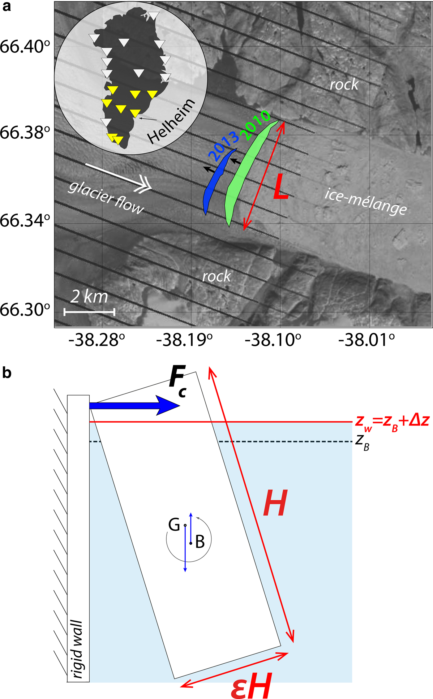
Fig. 2. Calved icebergs at Helheim glacier, GLISN seismic stations and geometry of the capsize model. (a) Locations of icebergs that calved on 10 July 2010, 17:49 UTC (green) and 25 July 2013, 03:13 UTC (blue), superimposed on Landsat 7 image from 10 July 2010. The iceberg surface projections are mapped from Murray and others (Reference Murray2015a) and James and others (Reference James, Murray, Selmes, Scharrer and OLeary2014). Black arrows indicate the horizontal direction of the forces inverted from glacial earthquake records at seismic stations shown in yellow triangles. (b) Schematic force balance (excluding drag forces and torques) acting on the 2-D iceberg (height H, along-glacier width εH) which tips over in bottom-out style in water with surface elevation z B + Δz, where z B is the water level for hydrostatic balance of the ice-block at the initiation of its capsize. Here the iceberg is super-buoyant as it experiences a positive Δz. The generated contact force F c is computed by integrating the normal stress on the calving face and is upscaled by the iceberg across-glacier length L.
Iceberg capsize model and contact forces
The iceberg capsize model of Sergeant and others (Reference Sergeant2018) is used to compute a catalog of contact forces. It solves the 2-D dynamic equations for solid mechanics and uses the finite-element description. The model accounts for various rheologies and can be easily expanded to glacier mechanics. In this study we restrict the model set-up to a simple configuration of icebergs capsizing bottom-out (i.e. the iceberg tips over counterclockwise in Fig. 2b) against a vertical wall which represents the fixed glacier calving front. It implies that basal sliding and elastic deformation of the glacier are neglected as well as its viscous flow, which should be negligible at calving timescales.
The model is 2-D and uses box-shaped icebergs with rectangular sections of height H and along-glacier width W. To be able to capsize, the iceberg aspect ratio ε = W/H has to be lower than a critical value which depends on the ice-to-water density ratio (MacAyeal and others, Reference MacAyeal, Scambos, Hulbe and Fahnestock2003). The iceberg is partly submerged in a ‘virtual layer’ that represents the surrounding sea water defined by the water level z w. The ice block then experiences the forces and moments exerted by gravity, buoyancy, water drag and contact reaction from the wall.
As nascent icebergs can be out of their hydrostatic equilibrium (e.g. James and others, Reference James, Murray, Selmes, Scharrer and OLeary2014; Murray and others, Reference Murray2015c), we control the water level to mimic various initial buoyancy conditions. The difference in water surface elevation experienced by the iceberg (z w) with respect to the theoretical one for an initially neutrally buoyant iceberg of the same geometry (z B) is denoted Δz. Icebergs which experience a negative Δz are then uplifted by buoyancy compared with their buoyant position at the initiation of the capsize. Conversely, for positive Δz, icebergs sink deeper.
The contact force generated on the terminus by the rotating iceberg is recovered by integrating the solid mechanics equation in time using the method of Hilber and others (Reference Hilber, Hughes and Taylor1977). A catalog of contact force historiesFootnote 1 is then computed with varying sets of (ε, H, Δz) values. The force generated by a 3-D ice block is computed using a scaling factor equal to the iceberg across-glacier length L. Possible contact forces are explored for iceberg geometries which describe typical Greenland glaciers. Iceberg volumes covered by the computed contact force catalog range between 0.018 and 4 km3 corresponding to parameters: 0.1 ≤ ε ≤ 0.6, 600 m ≤ H ≤ 1100 m, 500 m ≤ L ≤ 6000 m and − 20 m ≤ Δz ≤ 20 m.
ICEBERG VOLUME ESTIMATION FROM FORCE HISTORY
Horizontal GE force components are compared with the catalog of modeled contact forces, with the latter filtered in the same frequency band that was used for seismic inversion (20–100 s). The similarity of each pair of force time series is quantified via the variance reduction (VR) of their misfit. The calving volume inversion procedure consists of two steps. We first perform a (ε, H, Δz) parameter space exploration with a contact force catalog corresponding to a given iceberg length L i and calculate an iceberg volume V 0 given by a best-fitting aspect ratio ε0 and height H 0 as  $\epsilon _0 H_0^2 L_{\rm i}$. The uncertainty on the retrieved volume, noted δV 0, is computed from the variation of the misfit function on ε and H. This step is then repeated for every L and we compute the V 0(L) function which is then used to calculate and average a final iceberg volume V with statistical uncertainties, when consistent V 0(L i) values are obtained with L. All variables used in this study are reported in Appendix A.
Synthetic inversion of iceberg volumes and induced errors
We first run synthetic inversions to estimate the errors we could obtain on the iceberg volume with the first step of this procedure. We run several tests taking as input 20–100 s filtered contact forces which correspond to icebergs of various dimensions ε and H but one given length L and at hydrostatic balance (i.e. Δz = 0). We also investigate the dependency of the inversion results on the data force's signal-to-noise ratio (SNR). For one SNR, we average the errors on calculated iceberg volumes over 100 tests, each one taking as input a force that has been polluted by random noise which has the same dominant frequency.
For noise-free inversions, maximum VR is always reached for the exact input aspect ratio and height which then give correct volumes V 0 (Fig. 3a). When using noisy forces, maximum volume errors (15% for SNR=0.5 and 4% for SNR=5) are reached for the cases of intermediate aspect ratios. Depending on the tested geometry and notably the input aspect ratio, VR values decrease more or less fast around the maximum peak (Figs S2c and d). For each test, the volume uncertainty interval δV 0 plotted in Fig. 3b is constructed by taking all (ε, H) combinations that yield VR values >98% of maximum VR. While δV 0, as defined here, is always <15% for icebergs with ε ≤ 0.2, δV 0 increases up to 40% for intermediate ε due to wider distributions of high VR values. The variation of the contact force with iceberg dimensions is approximately symmetric about ε ≈ 0.4 (see Sergeant and others, Reference Sergeant2018, Fig. 6). The confidence interval on ε and H and therefore volume will then be higher and more difficult to reduce when the iceberg has an intermediate aspect ratio close to 0.4, as rather similar contact forces are observed around this value. The V 0 error or uncertainty δV 0 are then linked to the ability to discriminate contact forces with the aspect ratio, which can be even more difficult for poorly inverted data forces. Given the synthetic tests with the force SNR, in the worst case scenario, the maximum volume error would be 0.3 km3 for the biggest icebergs that a Greenland glacier is able to produce.
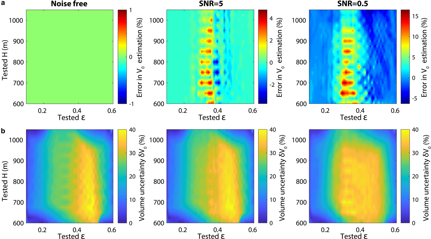
Fig. 3. Error on (a) estimated iceberg volumes and (b) associated confidence intervals from synthetic inversions run with 20–100 s filtered contact force histories for any iceberg of across-glacier length L=1. Synthetic tests are for noise-free input forces, and forces that have been polluted by random noise given a signal-to-noise ratio (SNR).
Validation study on two calving events at Helheim glacier
We illustrate the inversion process for two GEs that occurred at Helheim glacier. The associated calving events were captured on cameras, making it possible to estimate the iceberg dimensions (Fig. 2a). This section serves as a benchmark for our iceberg geometry calculations. One event (25 July 2013, 03:13 UTC) results from the capsize of an iceberg with a height equal to the full-glacier thickness H d ~ 800 m, an across-glacier length L d ~ 2500 m, and an aspect ratio εd ~ 0.23 (Murray and others, Reference Murray2015a). The iceberg volume was then estimated as 0.37 km3. The second event (12 July 2010, 17:49 UTC) results from the capsize of a 1.18 km3 iceberg with H d ~ 800 m, εd ~ 0.37 and 4000 m < L d < 5000 m (James and others, Reference James, Murray, Selmes, Scharrer and OLeary2014). The GE horizontal force components shown in Fig. 4a (blue and green lines) have maximum amplitudes of 3 × 10¹⁰ N and 4.6 × 10¹⁰ N for the 2013 and 2010 events, respectively.
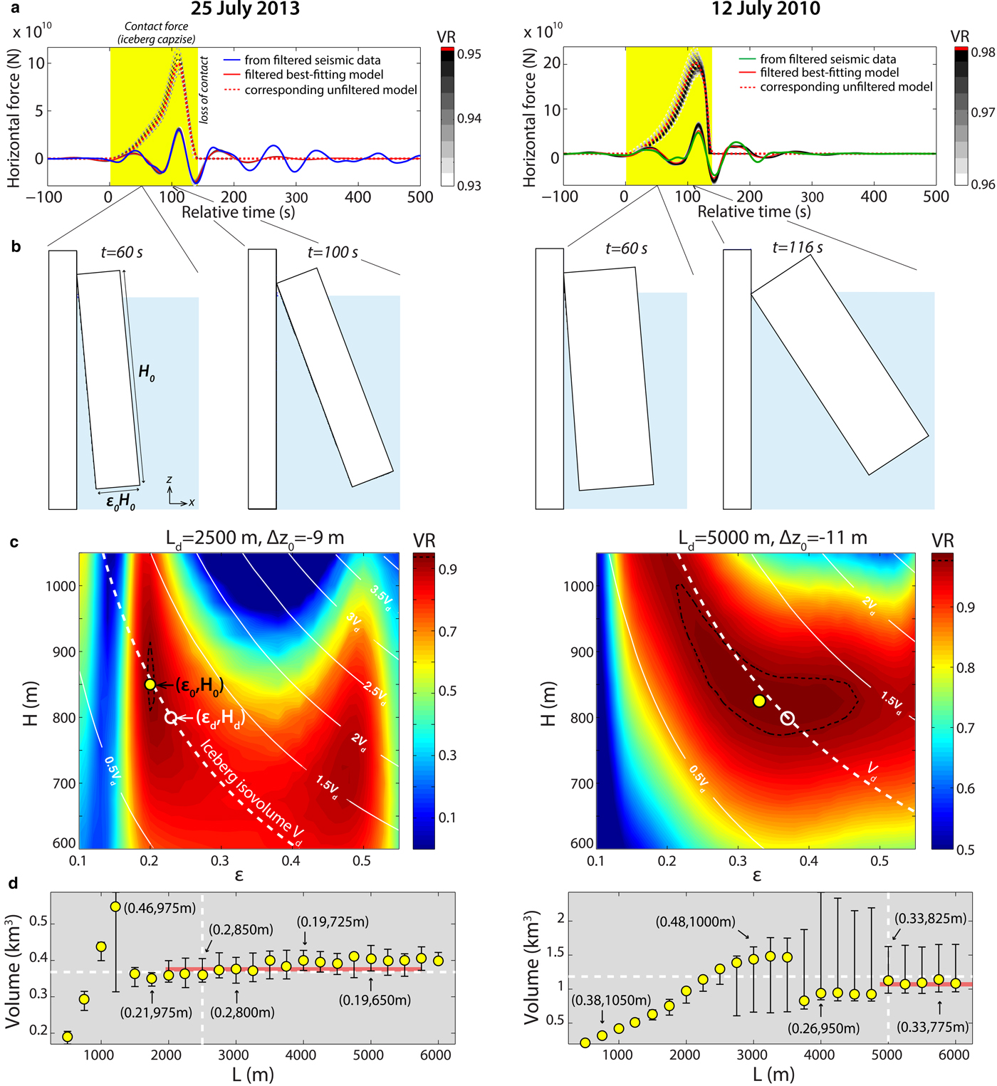
Fig. 4. Iceberg volume inversion for two well documented calving events of dimensions (εd, H d, L d). (a) Horizontal component of the force inverted from seismic data (blue or green for the 2013 and 2010 events, respectively) and associated best-fitting force models (red) bandpass filtered in the GE seismic band (20–100 s). Best force models correspond to parameters (ε0, H 0, Δz 0, L d) with the iceberg across-glacier length L d derived from field observations. Red dashed lines show the corresponding actual (i.e. unfiltered) contact force F c generated by the iceberg on the terminus. Grey-to-black shaded lines represent all force models that equivalently fit the seismic force with high variance reduction (VR) values. Yellow box indicates the iceberg-to-terminus contact duration. Snapshots of numerical simulations that are illustrated in (b). (c) Misfit function with iceberg dimensions ε and H for the catalog of contact forces scaled by the actual iceberg length (L = L d). For this representation, the third model parameter Δz has been fixed to the value reached for maximum VR, i.e. Δz 0 indicated above each panel. The real and calculated iceberg dimensions are (εd, H d) and (ε0, H 0), indicated by white and yellow-filled circles, respectively. The white lines show isovolumetric contours, when L is kept constant. (d) Computed iceberg volumes when varying L-values. White dashed lines indicate the actual iceberg length L d and volume V d. Uncertainties on estimated volumes are calculated from all (ε, H) combinations that yield VR values>98% of maximum VR, i.e. within the domain indicated by black dashed contour lines in (c). Derived iceberg dimensions (ε0, H 0) are indicated for some L-values. Beyond a critical iceberg length L, inverted aspect ratios and volumes are stable around correct values. The red thick line indicates the average calculated volume for the indicated L-range, i.e. when ε0 is stable and H 0 does not exceed ± 15% of the glacier thickness H d.
We first show in Fig. 4c the VR-misfit function with ε and H, obtained for L fixed to the actual iceberg length L d. Yellow-filled and white circles indicate best-fitting parameters (ε0, H 0) and true iceberg dimensions (εd, H d), respectively. For the 2013 event, the best VR value (0.95) is achieved for ε0 = 0.2, H 0 = 850 m and Δz 0 = −9 m. A negative Δz corresponds to an uplift of the ice block prior to its capsize which is well justified by the observations of Murray and others (Reference Murray2015c). For the 2010 event, maximum VR (0.98) corresponds to a 11 m-uplifted iceberg with ε0 = 0.33 and H 0 = 825 m. For both events, minimization-determined parameters are in good agreement with the true iceberg geometry and yield iceberg volumes V 0 of ~ 0.36 km3 and ~ 1.12 km3. Computed volumes are underestimated by <5%. While the volume uncertainty (illustrated by the black dashed line in Fig. 4c) is quite small (δV 0 < 7%) for the thinner iceberg, it increases up to 40% of V 0 for the larger calving event. Retrieved δV 0 intervals follow the same trend as observed with synthetic inversions with higher uncertainties obtained for intermediate aspect ratios. Finally, best-determined force models (red in Fig. 4a) reproduce the force data components well during the time period coincident to the capsize and indicated by the yellow box (Murray and others, Reference Murray2015a). Force models determined within the confidence interval (black-shaded lines) are very similar to the best-fitting force. They still show different force amplitudes which can also encompass amplitude uncertainties on the data forces that were obtained from GE records (Sergeant and others, Reference Sergeant2016).
The results of all inversion run with other L values are reported in Fig. 4d. Best retrieved parameters (ε0, H 0) and volumes V 0 vary with L, as L impacts the force amplitude to be matched. In a certain L range (indicated by red thick lines), the calculated aspect ratios and volumes are consistent and match the field observations, independently of the iceberg length. While the aspect ratio essentially controls the force time evolution and then gives consistent results over the L-fixed inversions, the force amplitude is more affected by the other iceberg dimensions as it is approximately proportional to H 3 and L (Tsai and others, Reference Tsai, Rice and Fahnestock2008; Amundson and others, Reference Amundson, Burton and Correa-Legisos2012a; Sergeant and others, Reference Sergeant2018). This means that for a given force, considering a well resolved ε as it is, a specific combination of decreased H and increased L values will result in the same iceberg volumes.
This analysis shows that, unless at least one dimension of the iceberg is known (as here L), it is difficult to invert all three individual iceberg dimensions (and then the iceberg geometry) from GE horizontal forces. However a volume can be robustly estimated when consistent results are obtained on a loop of inversions.
General inversion procedure for glacial earthquakes
The above procedure is applied to the forces computed for 203 GEs. Final calving volumes V are calculated as the average of all  $V_0=\epsilon _0H_0^2L_{\rm i}$ that are estimated for a given iceberg length L i, when accepted. This means that V 0, to be included in the final calculation of V, must (1) be stable around a certain value (i.e. V 0(L) function must have reached a plateau), while (2) ε0 is also stabilized and (3) H 0 does not exceed the actual glacier thickness ± 15%. In this study, we consider glacier thicknesses estimated in previous studies (e.g. Joughin and others, Reference Joughin2008a,Reference Joughinb, Reference Joughin, Smith, Shean and Floricioiu2014; Stearns and Hamilton, Reference Stearns and Hamilton2007; Howat and others, Reference Howat2011; Murray and others, Reference Murray2015c) or fixed to 800 m for most events. The latter condition (3) on the iceberg height is, in the end, not too restrictive as a maximum deviation of H 0 values of 15% of 800 m would nearly cover the entire range of investigated H given considered L range. The constraint on H and then V could be improved in future work by using bedmap data for Greenland (Griggs and others, Reference Griggs2012) or recent ice thickness measurements from IceBridge surveys (Rignot and others, Reference Rignot, Mouginot, Larsen, Gim and Kirchner2013). However the inversion results are consistent both with or without constraining H (Fig. S3). The final volume uncertainty δV for one event is computed as the quadrature propagated uncertainty
 $$\delta V = \displaystyle{1 \over N}\sqrt {\sum\limits_i^N {\delta V_0{(L_{\rm i})}^2} } $$
where δV 0(L i) is the uncertainty related to each of the N accepted models with given L i. We find δV uncertainties that vary between 0.01 and 0.33 km3 with 70% of the events reaching δV < 0.1 km3 (Fig. S4). The median value of δV is 0.07 km3 across all inverted GEs. This represents an average volume uncertainty of 6%.
RESULTS: ICEBERG PRODUCTION ASSOCIATED WITH GLACIAL EARTHQUAKES
Out of 15 GE producing glaciers in Greenland, seven are not included in this study as we fail to confidently determine GE sources and because not enough calving events could be characterized to make statistically relevant statements. We then focus our analysis on two Eastern major glaciers, Kangerdluqssuaq and Helheim, and six Western glaciers including Jakobshavn Isbrae, Rinks glacier and most active northwest glaciers, Upernavik Isström, Kong Oscar, Sverdrup, and Alison glaciers. Altogether, these glaciers cover 90% of the Greenland seismicity. Out of 203 GEs, the calving volumes of 28 events could not be estimated due to inconsistently calculated V 0(L) and large VR discrepancy. Finally, our sub-catalog of computed icebergs covers 40% of the total Greenland GE production and almost 45% of the production at considered glaciers.
As we aim to compute the evolution of capsizing calving volumes in Greenland and their contribution to the discharge, we need to assess the representativity of our sub-catalog of events. To do so, we look at the differences in magnitude patterns between our GE force database and the solutions for the complete event catalog. Fig. 5 shows the size-frequency distribution of GEs and computed calving volumes at each glacier. The proportion of inverted GEs with respect to the Nettles catalog varies from one glacier to another between 18 and 64% (Table 2, columns 1–3). Even if numerous events are missed (between 8 and 69 depending on the glacier), the distributions of the inverted seismic force amplitudes used in this study (F max, orange bars) cover the entire range of CSF magnitudes and resemble A CSF histograms of the Nettles catalog (blue bars). Our GE database covers almost every seismically active year at each glacier and no specific temporal trend in GE magnitudes is observed at individual glaciers (Veitch and Nettles, Reference Veitch and Nettles2012). This indicates that our sub-dataset would be representative of each glacier's overall seismicity in terms of temporal trend and GE sizes. It is worth noting that the two quantities that are compared, F max (with unit N) and A CSF (in kg m) have different natures and are obtained from different processing. We thus believe that discrepancies between the Nettles A CSF distributions and our F max is not necessarily related to incompleteness of our event sub-catalog.

Fig. 5. Size-frequency distributions of glacial earthquakes and inverted icebergs at individual Greenland glaciers for 1993--2013. Glacier locations are indicated in Fig. 8. Blue bars indicate CSF magnitudes A CSF from the Nettles catalog. Orange bars indicate the maximum amplitudes F max of the force time series that constitute our GE sub-catalog. Uncertainties on calving volume distributions come from the bin width (0.2 km3) used to generate histograms which is set to twice the median volume uncertainty obtained for all events.
Table 2. Characteristics of glacial earthquake (GE) production and associated discharge (GED) computed at Greenland glaciers. Columns give number of events, proportion of inverted events, most common CSF magnitude A CSF, most common inverted volume, GED in 1993–2013, and proportion of glacier dynamic discharge (DD) attributed to GEs for 2000–12. Columns 6–7 give results from GED median projections. Uncertainties are not reported here but are illustrated in Figs 7 and 12–14. GE contribution to the dynamic discharge DD averaged over East and West Greenland only accounts for DD measurements at the eight investigated glaciers.
Earthquake sizes and calving volumes
As noticed by Veitch and Nettles (Reference Veitch and Nettles2012), Greenland glaciers have different shapes of GE size distribution as measured by CSF. While every glacier's seismic activity shows a characteristic peak in magnitudes with a rapid decline at larger and smaller sizes of GEs, the peak occurs at different sizes depending on the source region (Fig. 5). The distribution width also varies from one place to another. Previous studies argue that the shape of GE size-frequency distributions is controlled by the glacier geometry with the upper bound of the magnitude being related to the biggest icebergs whose dimensions cannot exceed actual glacier thickness and width (Nettles and Ekström, Reference Nettles and Ekström2010; Veitch and Nettles, Reference Veitch and Nettles2012). As shown in Figs 5 and 6a–h, the biggest icebergs are observed at the largest glaciers Jakobshavn Isbrae, Kangedluqssuaq and Helheim where highest GE magnitudes A CSF are also recorded. The iceberg size-frequency distributions we obtain vary from one glacier to another and somehow follow the same evolution as for GE magnitudes, but not systematically at every calving site (Fig. 5). For example, the calving volume distribution at Kangerdlussuaq is wider than at Helheim as is the case for GE sizes, with a volume peak that is larger (1.5 km3) than Helheim's peak (0.7 km3). On the contrary, calving size distribution at Jakobshavn Isbrae shows a peak at 0.9 km3, which is larger than at Helheim, despite a smaller seismic magnitude peak. Even if all inverted calving volumes are actually below the maximum size of icebergs that each glacier is able to produce given the glacier width, the largest icebergs do not systematically correspond to the highest GE magnitudes as illustrated below.
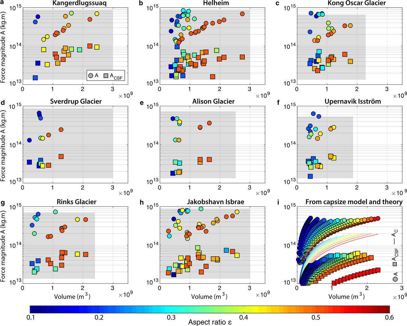
Fig. 6. Earthquake force magnitudes A CSF (squares) and associated contact force magnitudes A (dots) as a function of inverted calving volumes V at 8 Greenland glaciers (a-h). A CSF are obtained by seismic waveform inversion (Tsai and Ekström, Reference Tsai and Ekström2007; Veitch and Nettles, Reference Veitch and Nettles2012; Olsen and Nettles, Reference Olsen and Nettles2017). A are the magnitudes of actual contact forces (i.e. non-filtered) obtained when with our volume inversion method. Color indicates the inverted iceberg aspect ratio ε. Gray-shaded boxes denote an estimate of the range of possible iceberg size and corresponding force magnitudes A based on the geometry of the glacier terminus. For a comparison, synthetic evolutions of A CSF and A with iceberg volume and ε are presented in (i), as well as the evolution of the magnitude of the contact force A c ∝ H (1 − ε) V (Eqn (3), color lines) when hydrodynamic effects are neglected and H is fixed to 900 m.
Figure 6 shows the evolution of GE magnitudes A CSF (squares) with inverted volumes V , and associated actual contact force magnitudes A (dots, actually refer to non-filtered contact force models). Color indicates the iceberg aspect ratio ε calculated for each event. Comparing the dependence of A and A CSF on computed V at individual glaciers (Figs 6a–h) with the synthetic tests run with different iceberg sizes (Fig. 6i), the calving volumes we obtain for GEs yield reasonably good expected GE magnitudes. From this representation, we see that equivalent GE magnitudes A CSF can be reached for different sizes of icebergs and aspect ratios. These results tell us that the GE size-frequency distribution should not be interpreted in terms of exact calving volume distribution as GE magnitudes are dependent on the iceberg size, aspect ratio and height, collectively.
Mass loss related to glacial earthquakes and contribution to dynamic discharge
We now investigate the temporal evolution of the discharge associated with GEs over 1993–2013. To extrapolate the calving volume inversion results to the entire dataset of GEs which could not be characterized, we simply add to the iceberg catalog the most common ice volume that was calculated at each glacier (Table 2, column 5), when one seismic event was missed. This enables us to build the projected iceberg discharge we could expect if we had inverted the calving volumes for all GEs referenced in the Nettles catalog. Lower and higher expectations are built based on the smallest and biggest iceberg volumes that were inverted at each glacier. Results for individual glaciers and averaged over Greenland regions are shown in Figs 12–14 and Fig. 7, respectively. We will only discuss here the projected GE-associated discharge (called GED in the following). Annual and cumulated GED over the two decades are shown by blue bars and the blue line in Figs 7d–f.
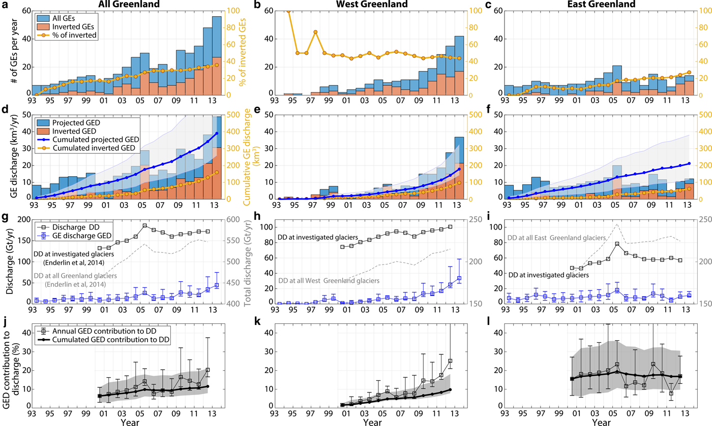
Fig. 7. Glacial earthquake (GE) and iceberg production across Greenland in 1993–2013. Evolution of (a–c) number of GEs, (d–f) associated calving volumes, (g–i) GE-associated discharge (GED, blue line) and dynamic discharge (DD, black line) at investigated glaciers and (j–l) GED contribution to DD in 2000--12. In (a–c) and (d–f), orange bars represent the number of GEs that were inverted in this study, and associated volumes; blue bars represent all GEs from the Nettles catalog and associated volumes that are expected based on the iceberg size-frequency distribution inverted at each glacier for the dataset in orange (Fig. 6). Right y-axis correspond to (a–c) the proportion of inverted GEs with respect to the Nettles catalog in the region and updated each year, and (d–f) cumulated GED based on inverted events only (yellow line), and based on expectations for all GEs (blue line) with their uncertainty (gray area). In (g–i), gray line (right y-axis) show dynamic discharge DD in the region when including also tidewater glaciers which did not produce GEs. Only eight GE-producing glaciers are accounted for in this study (Table 2). Details about GE production at individual glaciers are provided in Figs 12–14.
From our calculations, the eight glaciers included in this study produced between 270 km3 and 700 km3 with a median value of 398 km3 of ice (367 Gt equivalent) via GEs over the two decades 1993–2013. The biggest producers are Jakobshavn (71 km3), Helheim (86 km3) and Kangerdluqssuaq (117 km3). Altogether they account for half of the total GED we extrapolated for Greenland. While Eastern glaciers (Kangerdluqssuaq and Helheim) cumulated GED appears to have increased constantly over the whole time period, Western glacier mass loss has doubled since 2010 and thus contributes to the acceleration of Greenland GED since then. Before 2009, Western glacier annual GED never exceeded the average annual GED in East Greenland (i.e. 10 km3) and contributed to only 25% of the overall Greenland GED. In 2013, West Greenland GED exceeded the calving volumes produced by both Kangerdluqssuaq and Helheim cumulated over 2004/05 (i.e. 32 km3) when the two Eastern glaciers experienced a synchronous and fast retreat of more than 5 km, reaching their most retreated position ever recorded (Howat and others, Reference Howat, Joughin, Tulaczyk and Gogineni2005, Reference Howat, Joughin, Fahnestock, Smith and Scambos2008; Joughin and others, Reference Joughin2008a; Bevan and others, Reference Bevan, Luckman and Murray2012). Presently, the Greenland GED cumulated over 1993–2013 seems to have been equally partitioned between East and West regions (Table 2, column 6). If trends continue, the early dominance of Eastern glaciers is about to change notably due to a decrease in GE activity at Kangerdluqssuaq, which was the most productive Eastern glacier before its retreat, and most importantly to increasing GED contributions from Western glaciers including Jakobshavn and North West glaciers.
One concern is the contribution of buoyancy-driven calving to Greenland dynamic discharge (called DD in the following) which also includes submarine melting. Measurements from satellite imagery allow linear or areal frontal ablation rates to be determined, but it is rarely possible to measure the relative contribution of calving and melting below the surface (Benn and others, Reference Benn, Cowton, Todd and Luckman2017b). Because of these difficulties and the importance of glacier flow in governing rates of ice delivery to the terminus, DD is commonly quantified using measurements of the ice volume flux passing through a glacier cross-section. To estimate the proportion of GED to DD, we use DD measurements of Enderlin and others (Reference Enderlin2014) for years 2000–12. The GED generally follows the trend of DD (blue line versus black line in Figs 7g–i), except after 2010 when an acceleration of GED occurred at Western glaciers while the dynamic discharge observed in this area continued to increase constantly. We observe different levels of GE contribution to DD through time but also depending on the glacier and on the region (Table 2, column 7; Figs 7j–l). In 2012, Western glaciers experienced up to 25% of mass loss via GEs while the amount of GED tended to stabilize or even decrease when averaged over both Eastern glaciers, ~18%. In total, capsizing calving which produced earthquakes could have contributed between 8 and 21% of the discharge averaged over the Greenland glaciers included in our analysis, given the uncertainties on the projected calving volume time series. Including in our calculation every tidewater glacier in Greenland which is not observed to produce GEs (gray line in Fig. 7g), GED contribution to the GrIS discharge should be 3--4 times smaller, i.e. ~3--6% of Greenland mass loss (Table 3), although it is expected to account for more if trends continue.
Table 3. Contribution of glacial earthquake associated discharge (GED) to Greenland glacier dynamic discharge (DD) in 2000, 2005, 2012 and over 2000–12. Results (lower-upper bounds, median value is within brackets) in lines 1–2 are when (1) considering only the eight earthquake-producing glaciers for the calculation of DD, (2) when DD measurements account for every tidewater glacier in Greenland. Dynamic discharge data are from Enderlin and others (Reference Enderlin2014).
Spatio-temporal variability of calving activity
Results are summarized in Fig. 8 and averaged over four time periods. Cumulated calving volumes and their uncertainty are represented by the size of the black circles. Green dashed circles show GED contribution to the dynamic discharge DD at each glacier. Since the evolution of annual GE associated discharge is related to earthquake occurrences at one glacier, it is not possible with the former representation to assess whether the associated mass loss is accelerating through more frequent events or through larger volumes per event, or both. We therefore introduce the cumulative GE-associated discharge anomaly C defined as
 $$C=\sum_k^N (V_k - \lt V\gt)$$
where V k denotes iceberg volumes associated with N GEs within a given time period (e.g., 1 year) at one glacier, and < V > is the mean iceberg volume, averaged over all events produced at the glacier between 1993 and 2013. For constant discharge, C ≈ 0. C>0 (red colors in Fig. 8) when bigger icebergs are produced over one time period, on average. Conversely, C<0 (blue colors) when produced icebergs were smaller than usual. C results are similar whether they are computed on projected iceberg volume time series or on volumes which were actually inverted from GE records. This supports the argument that our calculations of discharge expected for the complete Nettles catalog did not introduce any bias in the analysis that follows.
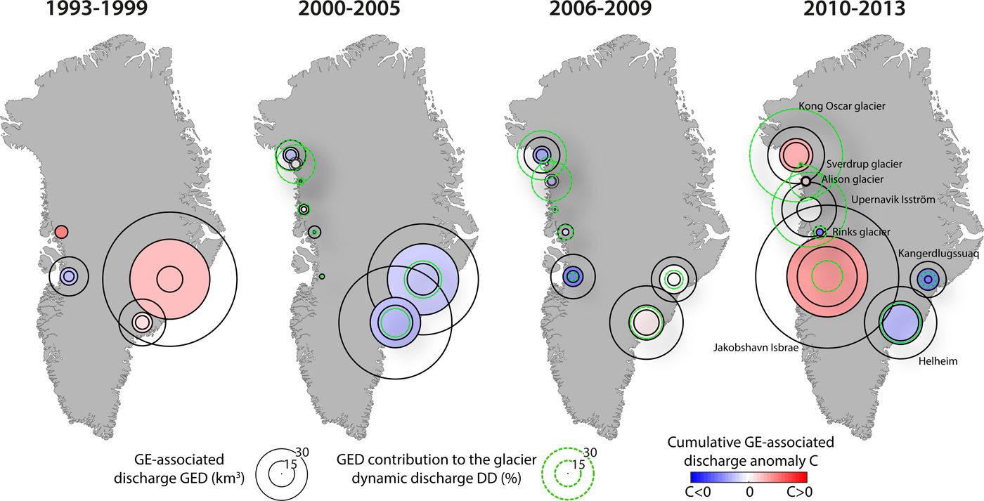
Fig. 8. Evolution of calving volumes with lower and upper uncertainties (black circles) that were produced at individual glaciers in Greenland through glacial earthquakes (GEs) for four time periods. Inner color of circles indicate value of the cumulative GE-associated discharge anomaly C at the considered time period. Red colors (C > 0) indicate that single glaciers discharge bigger icebergs with respect to their average size calculated over 1993–2013, and blue colors (C < 0) indicate that GE-associated discharge happens through more but smaller individual events. Conversely, white color (C ~ 0) indicates when glaciers produce icebergs of approximately constant sizes, compared to the average size over the whole time period. GE contributions to the glacier dynamic discharge DD in each period of time are indicated by the size of green circles. Iceberg production is only represented at glaciers where enough GEs (> 15% of the GE production) could be inverted.
Western glaciers
As observed by Veitch and Nettles (Reference Veitch and Nettles2012) and Olsen and Nettles (Reference Olsen and Nettles2017), GE production has increased since the early 2000s while Greenland glaciers accelerated during a period of above-average oceanic and atmospheric temperatures (Rignot and others, Reference Rignot2004; Holland and others, Reference Holland, Thomas, De Young, Ribergaard and Lyberth2008; Murray and others, Reference Murray2010; Straneo and others, Reference Straneo2010; Bevan and others, Reference Bevan, Luckman and Murray2012). North West Greenland was also affected with an increased number of glaciers which began to retreat and accelerate. The fresh occurrence of GEs in North West Greenland is then likely related to changes in sea-ice and ice-mélange buttressing strength, glacier speeds, thinning rates and any successions of advancing and retreating phases (Moon and Joughin, Reference Moon and Joughin2008; Moon and others, Reference Moon, Joughin and Smith2015; Joughin and others, Reference Joughin, Smith, Howat, Scambos and Moon2010; Howat and Eddy, Reference Howat and Eddy2011; McFadden and others, Reference McFadden, Howat, Joughin, Smith and Ahn2011; Carr and others, Reference Carr, Vieli and Stokes2013) which may have brought the glacier calving fronts to near-grounded positions, facilitating seismogenic buoyancy-driven calving (Amundson and others, Reference Amundson2010). The growing numbers of GEs in West Greenland suggest that these glaciers still approach near-grounded and floating positions each year, mostly in summer (Olsen and Nettles, Reference Olsen and Nettles2017). While before 2010, most discrete calving volumes were still small (i.e. C<0), it appears that iceberg sizes in this region tend to become larger also contributing to accelerated mass loss on the Western coast.
Eastern glaciers
On the contrary, GE production globally decreased in South Eastern Greenland after 2005 as Helheim and Kangerdluqssuaq stabilized after retreat (Bevan and others, Reference Bevan, Luckman and Murray2012). Nevertheless, differences occur between the two glaciers. While GE-associated discharge has been sustained at Helheim with successive periods of bigger and smaller iceberg release (Fig. 9b), Kangerdluqssuaq production in terms of events, iceberg sizes and GED contribution to discharge DD has been decreasing since 2006 and particularly 2011 (Fig. 9d). Since 2005, GEs have been active at Kangerdluqssuaq only during retreat phases when the glacier retreated toward specific positions in the fjord and accelerated (Fig. 9c), suggesting that terminus position and glacier speed play an essential role in capsizing calving. By 2011 as a consequence of sustained thinning (Howat and Eddy, Reference Howat and Eddy2011), Kangerlussuaq's grounding line had retreated into shallower water and remained stable as the glacier developed a 5 km-long floating ice-tongue, affecting its calving behavior (Kehrl and others, Reference Kehrl, Joughin, Shean, Floricioiu and Krieger2017). Since 2011, we observe smaller calving events at Kangerdluqssuaq which contrasts with the 2005–13 calving behavior at Helheim which had maintained a lightly grounded terminus (James and others, Reference James, Murray, Selmes, Scharrer and OLeary2014; Kehrl and others, Reference Kehrl, Joughin, Shean, Floricioiu and Krieger2017).

Fig. 9. 1993–2013 front positions (orange) and speed (black) at (a) Helheim, (c) Kangerdluqssuaq and (e) Jakobshavn. Vertical bars indicate timing of glacial earthquakes (GEs). (b, d, f) Evolution of the cumulative GE-associated discharge anomaly C at corresponding glacier. 1993–2011 Eastern glacier positions are from Bevan and others (Reference Bevan, Luckman and Murray2012) and updated to 2013. 2009–13 Jakobshavn pos: itions are from Joughin and others (Reference Joughin, Smith, Shean and Floricioiu2014).
Links to glacier dynamics
To link calving patterns to ice flow dynamics, we analyze the evolution of calculated calving volumes with glacier speed and front position at Jakobshavn and Helheim. Jakobshavn Isbrae, while retreating, has continuously produced GEs since 2005 (Figs 9e and f) after the disintegration of a 15 km-long floating tongue (Joughin and others, Reference Joughin, Abdalati and Fahnestock2004). Between 2009 and 2013, the annual number of seismic events and related discharge has almost tripled and as previously reported, the average trend has produced bigger calving events. If we look at the dependency of GE production and calving volumes on ice flow speed and glacier geometry (Fig. 10), we observe that the largest icebergs calve at maximum speeds (i.e. 15 km a−1) and at specific terminus positions (i.e. 10–11 km relative to the reference point in the along-flow profile in Joughin and others, Reference Joughin, Smith, Shean and Floricioiu2014). In 2009–13, Jakobshavn remained near-grounded as the calving front was resting over a bed depression (Joughin and others, Reference Joughin, Smith, Shean and Floricioiu2014). In July--September 2012/13 (orange and dark red data points), the glacier reached its most retreated position at greatest water depths coinciding with highest flow speeds, largest icebergs and also fewest calving events. As a terminus with little or no floating extension advances into deep water and approaches buoyancy, hydrostatic imbalance at the front causes downward bending (Wagner and others, Reference Wagner, James, Murray and Vella2016). This initially prevents the ice from attaining buoyant equilibrium and buoyant flexure of the terminus must be balanced upstream by enhanced longitudinal stress. This can lead to glacier stretching and acceleration (Nick and others, Reference Nick, Vieli, Howat and Joughin2009; Joughin and others, Reference Joughin2012, Reference Joughin, Smith, Shean and Floricioiu2014) and the development of a super-buoyant tongue whose length increases as ice advances (Benn and others, Reference Benn2017a). It can become several hundreds of meters long before buoyant forces are high enough to initiate calving. Our observations of increased calving sizes with deeper water and increased flow velocity agree with modeling results for glacier retreat behavior over a reverse bed slope (Nick and others, Reference Nick, Vieli, Howat and Joughin2009) or glacier advance in deepening water (Wagner and others, Reference Wagner, James, Murray and Vella2016). A similar analysis can be done for Helheim calving production (Fig. 11): as the glacier was retreating over a reverse bed slope in 2004/05, it reached its most retreated position in deeper water in 2005 (green data points) producing bigger iceberg sizes; since that time it has alternated advance and retreat phases over the bed overdeepening producing a wide range of calving events.
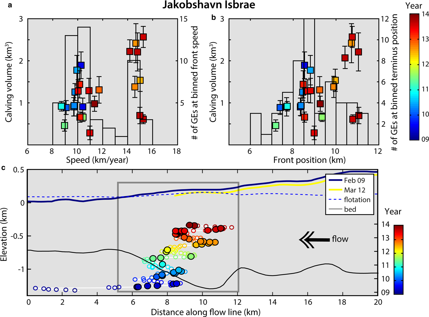
Fig. 10. Evolution of 2009–13 GE and calving production with Jakobshavn's geometry (i.e. along the southern ice-stream). Number of detected GEs (bars) and associated calving volumes (color squares) as a function of terminus (a) speed and (b) front position along the profile described in Joughin and others (Reference Joughin, Smith, Shean and Floricioiu2014). Color indicates relative time since1 January 2009. In (c) color circles indicate front positions relatively to time. Filled circles indicate GE-active periods (i.e. mostly in summer). Bed topography is in black. Blue dashed line indicates the flotation threshold, above which the ice should be grounded and below which the glacier is super-buoyant (i.e. deeper than buoyant equilibrium). Glacier surface elevation profiles are plotted for February 2009 and March 2012. Gray box indicates the magnified region in (b). Glacier geometry-related data are from Joughin and others (Reference Joughin, Smith, Shean and Floricioiu2014).
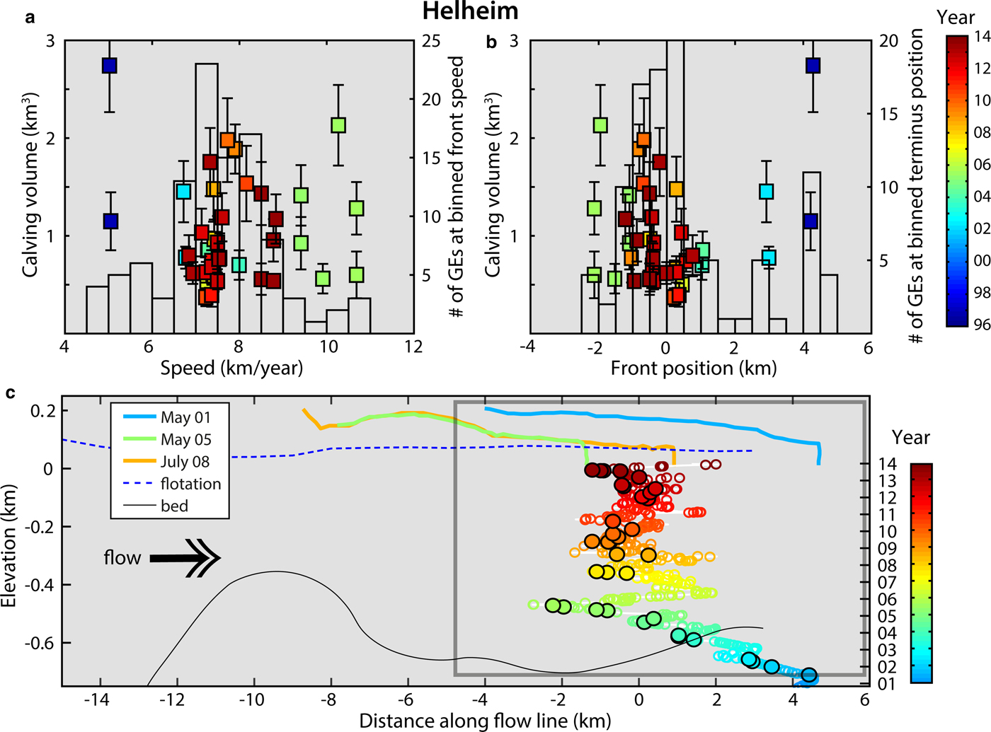
Fig. 11. Same as in Fig. 10 for 1996–2013 calving production at Helheim glacier. 1996–2011 calving front positions are from Bevan and others (Reference Bevan, Luckman and Murray2012) and updated to 2013. Glacier geometry in (c) is from Kehrl and others (Reference Kehrl, Joughin, Shean, Floricioiu and Krieger2017).
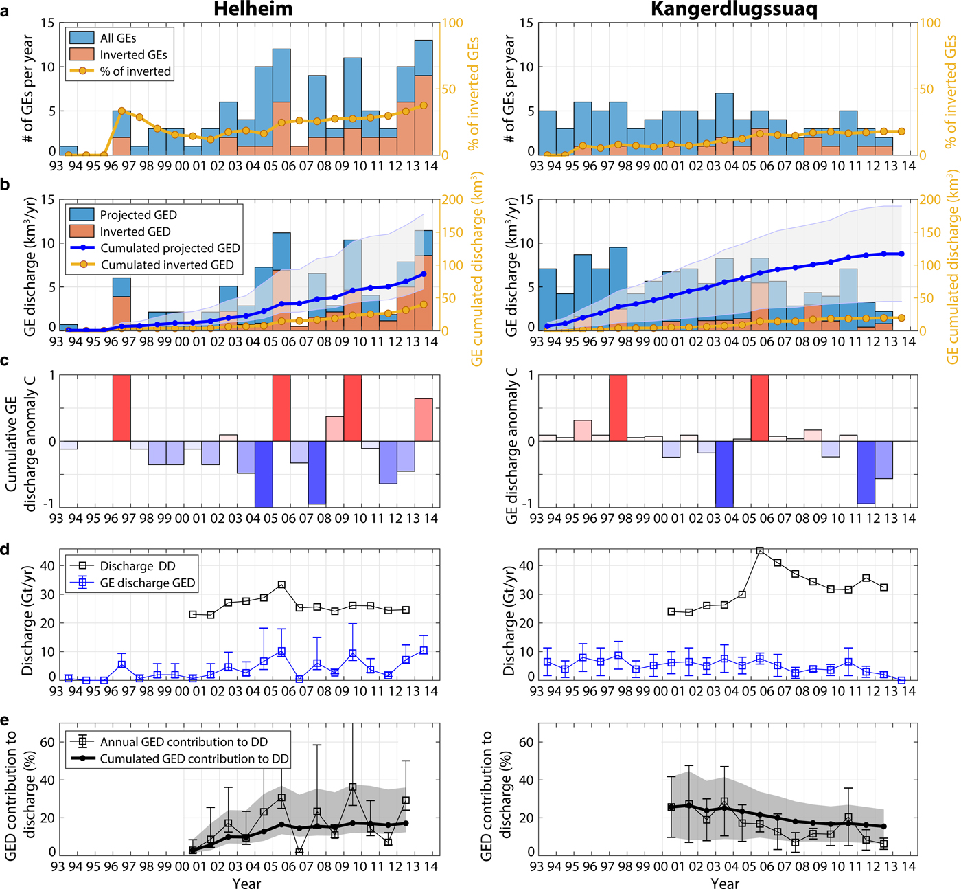
Fig. 12. GE and iceberg production at Helheim and Kangerdluqssuaq (South East Greenland) in 1993–2013. Evolution of (a) number of GEs, (b) associated calving volumes, (c) cumulative GE-associated discharge anomaly C, (d) GE-associated discharge (GED, blue line) and dynamic discharge (DD, black line) from Enderlin and others (Reference Enderlin2014), (e) GED contribution to DD. In (a) and (b), orange bars represent the number of GEs that were inverted in this study, and associated volumes; blue bars represent all GEs from the Nettles catalog and associated volumes that are expected based on the iceberg size-frequency distribution inverted at each glacier for the dataset in orange (Fig. 6). Right y-axis correspond to (a) the proportion of inverted GEs with respect to the Nettles catalog in the region and updated each year, and (b) cumulated GED based on inverted events only (yellow line), and based on expectations for all GEs (blue line) with their uncertainty (gray area).
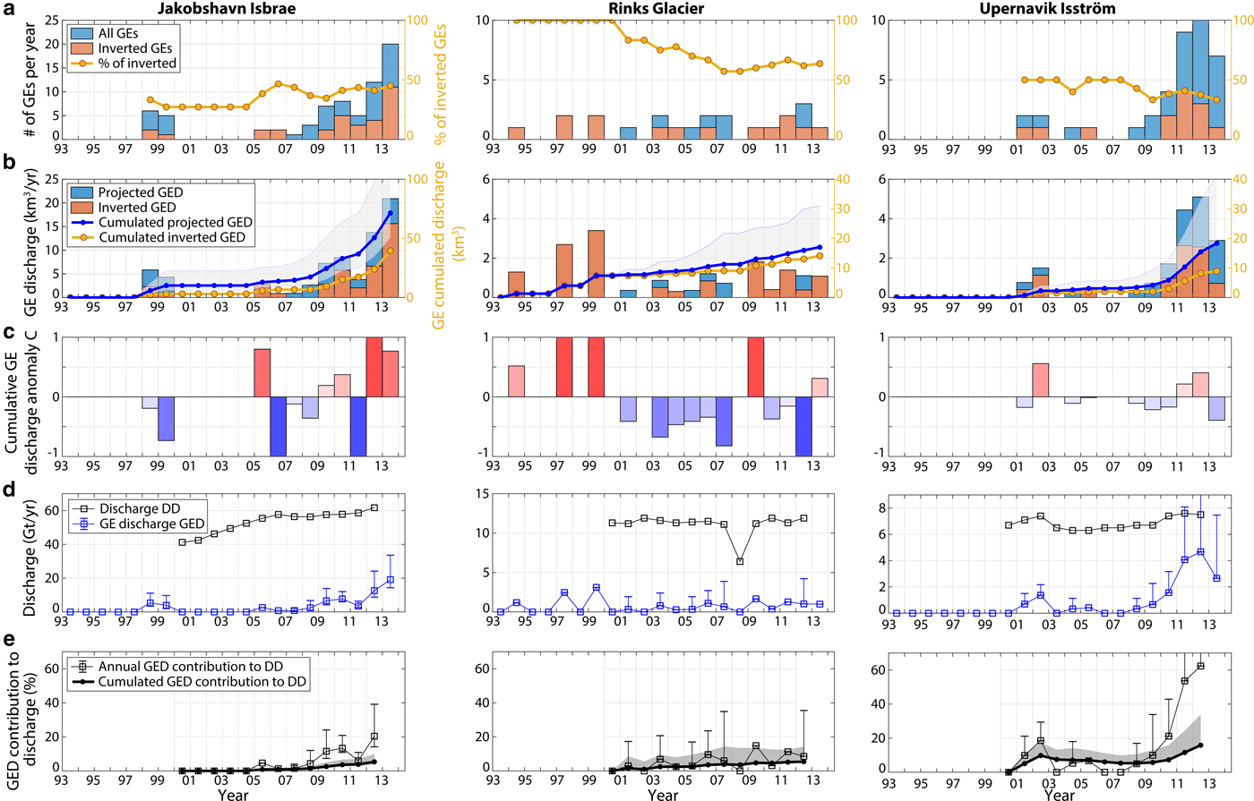
Fig. 13. Same as in Fig. 12 for Jakobshavn Isbrae, Rinks glacier and Upernavik Isström (West Greenland).
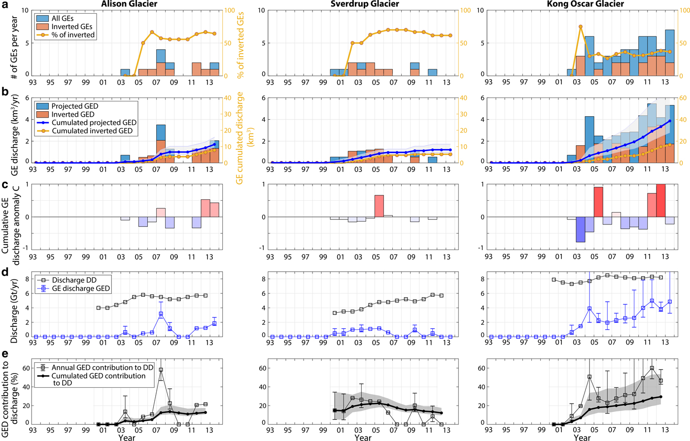
Fig. 14. Same as in Fig. 12 for Alison, Sverdup and Kong Oscar glaciers (North West Greenland).
GEs and calving patterns depend on the terminus front position which determines the flow speed and flotation level (Nick and others, Reference Nick, Vieli, Howat and Joughin2009; Joughin and others, Reference Joughin, Smith, Shean and Floricioiu2014). The tendency of a glacier to produce full-glacier thickness capsizing icebergs is related to the exploitation of existing basal crevasses which tend to develop in the vicinity of the grounding line (Van der Veen, Reference Van der Veen1998). Murray and others (Reference Murray2015c) suggest that the propagation of crevasses to the glacier surface is strongly enhanced when the glacier base is deeper than buoyant equilibrium. This condition was met at Jakobshavn Isbrae in 2009–13 and at Helheim since 2004/05, as both glaciers were retreating and advancing over a basal depression. Since 2005, most northwestern glacier retreat has been accelerating (McFadden and others, Reference McFadden, Howat, Joughin, Smith and Ahn2011; Carr and others, Reference Carr, Vieli and Stokes2013; Moon and others, Reference Moon, Joughin and Smith2015) followed by increasing occurrences of GEs and calving volumes since 2010. Such changes in calving behavior may then be related to fresh new boundary conditions as the termini have to reach near-grounded positions and could approach near-floating and deep water conditions.
DISCUSSION
Calving volume inversion from glacial earthquakes
We have demonstrated that estimating robust calving volumes from GE force history is possible when averaged over consistent iceberg inversion results (i.e. V 0(L)). The fact that we fail to constrain iceberg shape (i.e. all three individual dimensions) does not result from our processing. It would rather be due to the difficulty to distinguish very similar contact forces that can be generated by capsizing icebergs of different geometry, and especially different height and length. Due to the symmetrical nature of the contact force amplitudes around ε ~ 0.4 (Sergeant and others, Reference Sergeant2018), the comparison between seismic and modeled force histories for one given L may give two peaks of the misfit function in the case of icebergs with a small aspect ratio or conversely, a large aspect ratio. For the 2013 Helheim event presented in Fig. 4c, we obtain two regions of a similar force fit, around ε = 0.2 and ε = 0.47 corresponding to VR values of 0.98 and 0.9, respectively. Volume error associated with the secondary VR peak would be 66% of the true value. Although the difference between the extreme VR peak values may be small, the best force model is always achieved in the right ε region as shown by synthetic inversions of calving volumes, even when noisy forces are considered (Fig. 3). The ambiguity in the iceberg volume is therefore possible to be resolved thanks to the aspect ratio's control on the force history.
In the following we discuss the errors we could obtain when trying to fit a calving volume to the earthquake magnitude A CSF. Considering non-deforming icebergs and glacier termini, the contact force magnitude A can be expressed as the sum of a geometric term A c which comes from the (twice-)integrated contact reaction, and a hydrodynamic term A w. A w comes from the integration of drag forces and forces that arise from water pressure gradients that may be created by water deflection during iceberg tipping. The analytical form of A w is difficult to assess, though numerical modeling of drag forces (Amundson and others, Reference Amundson, Burton and Correa-Legisos2012a; Sergeant and others, Reference Sergeant2018) and hydrodynamic fields (Bonnet and others, Reference Bonnet2018) show that accounting for water effects is critical for capturing capsize dynamics. However, following Tsai and others (Reference Tsai, Rice and Fahnestock2008) and Amundson and others (Reference Amundson, Burton and Correa-Legisos2012a, see equation 19), when neglecting hydrodynamics effects and considering thin enough icebergs (ε < 0.5), the contact force magnitude A would be equal to A c which scales as
 $$A_{\rm c}\approx \displaystyle{1 \over 2}\rho _{\rm i}H(1-{\rm \epsilon })V,\quad {\rm when}\;{\rm \epsilon } < 0.5$$
where ρ i is the density of the ice. The central question is, if we assume the iceberg height H to be equal to the full glacier thickness H d we could deduce from additional glaciological measurements, is it possible to derive an appropriate scaling factor between GE magnitudes and calving volumes ? If thin icebergs are considered (i.e. 1 − ε ~ 1), A c/V would be of the order of 106 kg.m−2. However, any variation in ε alone may cause variations in the A c/V scaling factor of one order of magnitude leading then to errors in estimated volumes which can reach up to 1 km3 when trying linear regressions between A CSF and V (see also volume deviations with ε for same A c quantities in color lines, Fig. 6i). Then the extrapolation of GE magnitudes to calving volumes is difficult without high uncertainties. The comparison of GE force histories with adapted mechanical modeling of contact forces is then needed to extract accurate calving volumes.
One control on the time evolution of the contact force is the parameter couple (ε, Δz). Quantifying the influence of Δz relative to the one of ε or other iceberg dimension on the inversion results is not straightforward. Buoyant flexure of the glacier plays a significant role in calving (Wagner and others, Reference Wagner, James, Murray and Vella2016). Glacier elevation with respect to flotation level varies with the distance to the grounding line, and is sensitive to glacier thickness, glacier flow and water depth. The physical meaning of parametrization Δz used here is not straightforward to link to glacier flotation level. Indeed the elevation of the nascent iceberg (captured in Δz) is not necessarily the same as for the glacier beam as it depends also on the shape of the iceberg submerged part. To better describe iceberg and glacier buoyancy states, more complex models which deal with viscous ice flow and subglacial topography including the complex crevasse network need to be used. Therefore, exact values of calculated Δz are difficult to integrate into our analysis. Nevertheless, the most inverted Δz describe uplifted icebergs (Fig. S3c). This result is reasonable and corresponds to observations of calving dynamics at Helheim (Joughin and others, Reference Joughin2008a; James and others, Reference James, Murray, Selmes, Scharrer and OLeary2014; Murray and others, Reference Murray2015c).
We were not able to compute the calving volumes of 14% of the 203 inverted GEs as no consistent volumes were reached when varying L. In this study we used a catalog of contact forces for bottom-out capsizes only. As hydrodynamics affect top-out and bottom-out capsizes differently, contact forces differ with calving style (Amundson and others, Reference Amundson, Burton and Correa-Legisos2012a; Sergeant and others, Reference Sergeant2018). Such deviations may justify our viability to invert coherent iceberg parameters for a portion of the events. Indeed, top-out events are observed to be much less frequent in nature than bottom-out icebergs (Amundson and others, Reference Amundson2010). The discrimination between top-out and bottom-out events is difficult when only based on the horizontal seismic force. Further modeling efforts including real glacier terminus conditions should help to better distinguish between calving styles, when using also the capsize-generated vertical forces in the inversion procedure.
Representativity of calving discharge
The estimation of Greenland discharge attributed to buoyancy-driven calving is reliable only if (1) our subset of seismic events is statistically representative for Greenland glacier seismicity as discussed in the previous sections, and if (2) the Nettles catalog of GEs itself is also representative of capsizing calving in Greenland. In the following we discuss this further.
Seismic detection of nontabular iceberg calving
Since they have been studied routinely, GE datasets have been complemented with different versions of the detection algorithm. Including regional Greenland stations in the detection process improved earthquake detections (Veitch and Nettles, Reference Veitch and Nettles2012; Olsen and Nettles, Reference Olsen and Nettles2017). However, many studies which use concurrent observations such as time-lapse photography, satellite imagery, local seismometers, or even water pressure sensors near the glacier report numerous capsizing calving events which remained undetected by standard processing (e.g. Amundson and others, Reference Amundson2010, Reference Amundson2012b; Walter and others, Reference Walter, Olivieri and Clinton2013). For example, Kehrl and others (Reference Kehrl, Joughin, Shean, Floricioiu and Krieger2017) observed in the fjord of Helheim glacier ~70 nontabular icebergs between 2008 and 2013 while only 37 GEs were detected. Olsen and Nettles (Reference Olsen and Nettles2018) use cross-correlation templates at regional stations to identify smaller calving events (0.04–0.3 km3 measured from satellite imagery) which did not pass the detection threshold on teleseismic data. Olsen and Nettles (Reference Olsen and Nettles2018) estimate that undetected events could represent ice loss totaling an additional 10% of that accounted for by the glacial-earthquake standard catalog.
Calving discharge
We estimated the volume of ice discharged in Greenland through GEs in 1993–2013 to be 398 km3 with lower and upper bounds being 270 km3 and 700 km3, respectively. Disparities between lowest, highest and median GED expectations come from the shape of the iceberg size-frequency distributions at individual glaciers and are difficult to reduce due to our analysis of a limited number of GEs. As outlined with Figs 9–11, the interannual variability of calving volumes is related to glacier geometry and buoyant state, flow velocity and ice-front position. When a glacier experiences large fluctuations in its fjord position from one year to another and speed acceleration, the annual average and predominant calving volume should shift. Estimates of GE-associated discharge could then be refined when averaged over different timescales.
Calving discharge was not calculated at seven glaciers which produced altogether 46 GEs (i.e. 10% of Greenland GE production). As predominant calving volumes vary from one glacier to another, it is difficult to assess the amount of GE-associated discharge that is missed in our study.
Finally, as discussed above, our calculated discharge (Tables 2 and 3) should give a lower bound to the discharge that is attributed to capsize events in Greenland. Besides, tidewater glaciers also produce numerous km-scale tabular icebergs and smaller icebergs which fall from ice cliffs or detach from underwater ice protrusions (Rignot and others, Reference Rignot, Fenty, Xu, Cai and Kemp2015; Wagner and others, Reference Wagner, James, Murray and Vella2016). It is then expected that calving is responsible for a much larger part of the GrIS dynamic mass loss.
SUMMARY AND CONCLUSIONS
We developed a seismo-mechanical procedure for calculating calving volumes of seismogenic buoyancy-driven calving events which generate GEs in Greenland. The use of passive seismology is on its way to become a standard tool for investigating glacier processes and monitoring glacier changes (Podolskiy and Walter, Reference Podolskiy and Walter2016; Aster and Winberry, Reference Aster and Winberry2017). This study shows that for calving-related seismicity, classical seismic quantities such as the earthquake magnitude are difficult to interpret in terms of glaciological processes and mass loss as the seismic source is influenced by sea/ice interactions, iceberg and glacier geometries and hydrodynamic effects (Amundson and others, Reference Amundson, Burton and Correa-Legisos2012a; Sergeant and others, Reference Sergeant2018; Bartholomaus and others, Reference Bartholomaus, Larsen, O'Neel and West2012, for small non-capsizing icebergs). In the case of GEs and capsizing icebergs, the magnitude of the seismic source force cannot be used to uniquely define iceberg volumes, without errors of the order of 1 km3.
To refine the quantification of calving volumes, we propose to use the force history which captures the capsize dynamics that are primarily controlled by the iceberg shape. Whereas all three dimensions of icebergs are difficult to resolve well without any a priori postulation on at least one of them, iceberg volume can still be inverted. Indeed a robust calving volume can be estimated by averaging consistent inversion results run for several sets of iceberg dimensions. The confidence interval on the iceberg size varies with the iceberg geometry and can reach up to 40% for icebergs with intermediate width-to-height ratios. Synthetic tests give a maximum error on estimated volumes of 15% when run on poorly inverted force time series, which represents 0.3 km3 for the largest Greenland capsizing icebergs. We confidently inverted the iceberg sizes of ~ 200 capsizing events with an average uncertainty of 6% of the calving volumes.
We calculated the calving volumes of 40% of all GEs that were referenced in Greenland between 1993 and 2013. Thanks to preferred iceberg size-frequency distributions at individual glaciers, we could extrapolate the results to complete time series of GE-associated discharge at eight tidewater glaciers. Despite large uncertainties that are difficult to reduce due to our limited GE analysis, the total mass loss related to such events was estimated to be at least ~ 250 Gt (most probable value 367 Gt) over 1993–2013. While the iceberg discharge cumulated over the two decades has been so far equally partitioned between East and West Greenland, the contribution of Western glaciers has been accelerating since 2010 with an increasing number of calving events (Olsen and Nettles, Reference Olsen and Nettles2017), but also increasingly larger produced icebergs. The comparison between ice-front position, GE occurrence and iceberg size indicate that glacier produced larger icebergs when they were advancing into deepening water. While the increasing numbers of GEs and related discharge that are observed since the early 2000s follows the general trend of widespread glacier acceleration, retreat, increased calving rates and discharge across Greenland, the variability in GE and calving production over time and space is to be related to the glacier geometry control on ice flow dynamics.
One third to one half of GrIS mass loss has been attributed to dynamic discharge at outlet tidewater glaciers, including calving and submarine melting. We estimate that buoyancy-driven calving events that produced GEs could be responsible for 8 to 21% of the total discharge recorded at the same glaciers (most probable value 12%) and between 3 and 6% of the overall ice-sheet loss. These estimations do not include other types of calving such as tabular icebergs and smaller icebergs. A large number of capsizing events which have produced earthquakes but remained undetected by the standard algorithms has recently been reported (e.g. Kehrl and others, Reference Kehrl, Joughin, Shean, Floricioiu and Krieger2017). This implies that our calculations on the contribution of such calving events to the Greenland mass loss could be far underestimated (at least 10% according to Olsen and Nettles, Reference Olsen and Nettles2018). At Western glaciers, ice discharge through GEs has accelerated more rapidly than dynamic mass loss at the same glaciers. If trends continue and tidewater glaciers keep their near-grounded positions, buoyancy-driven calving and calving in general could become a major component of the GrIS mass loss.
We have illustrated in this study that GEs can help to quantify the partitioning of Greenland mass loss and monitor tidewater calving behavior which is crucial for a better representation of calving processes (Benn and others, Reference Benn2017a). Improvements in seismic detections and characterization of GEs are needed to expand the results of this study to a complete catalog of seismic and calving events. For a decade, increasingly high rate measurements of glacier characteristics and dynamics (e.g. James and others, Reference James, Murray, Selmes, Scharrer and OLeary2014) have been collected. Reverse motion and acceleration of the glacier trunk were observed during and after capsize events (Murray and others, Reference Murray2015a; Rosenau and others, Reference Rosenau, Schwalbe, Maas, Baessler and Dietrich2013; Holland and others, Reference Holland2016). The dynamics have been so far attributed to ice elastic deformation under capsizing iceberg forces (Murray and others, Reference Murray2015a) and viscous flow adjustment to the loss of resistive stress at the terminus front (Howat and others, Reference Howat, Joughin, Tulaczyk and Gogineni2005; Joughin and others, Reference Joughin2008a). The processes controlling glacier adjustment to calving are still not resolved. They could involve frictional sliding or stick-slip events as observed in Antarctica (Bindschadler and others, Reference Bindschadler, King, Alley, Anandakrishnan and Padman2003; Winberry and others, Reference Winberry, Anandakrishnan and Alley2009). Coupling sophisticated models of glaciers with glaciological and seismic measurements offer a high potential for characterizing calving processes at tidewater glaciers and basal processes which are key unknowns for future sea-level rise estimation (Ritz and others, Reference Ritz2015).
SUPPLEMENTARY MATERIAL
The supplementary material for this article can be found at https://doi.org/10.1017/aog.2019.7
ACKNOWLEDGMENTS
The numerical modeling was done using Z-set (www.zset−software.com), a non-linear finite-element suite developed by the Centre des matériaux, Mines ParisTech and Onera (France). Seismic stations used in this study are part of the Greenland Ice-sheet Monitoring Network (Anderson and others, Reference Anderson2009) and seismic records can be accessed through IRIS data center (www.iris.edu). Seismic data were collected via ObsPy routines. Figures in this paper were created with Matlab. We acknowledge Douglas MacAyeal as the scientific editor and two anonymous reviewers who helped to improve the quality of the manuscript. We thank Meredith Nettles and Kira Olsen for providing the catalogs of seismic events (www.globalcmt.org/Events), Ellyn Enderlin who kindly shared ice discharge data, Clément Hibert and Guillaume Jouvet for fruitful discussions. This work and authors have been partially funded by the ANR contract ANR-11-BS01-0016 LANDQUAKES; CNCS-UEFISCDI project PN-II-ID-PCE-2011-3-0045, Institut Universitaire de France; the ERC contract ERC-CG-2013-PE10-617472 SLIDEQUAKES; the Swiss National Science Foundation for project GlaHMSeis PP00P2-157551; and a DGA-MRIS scholarship. This is IPGP contribution 4024.
Appendix
Notations


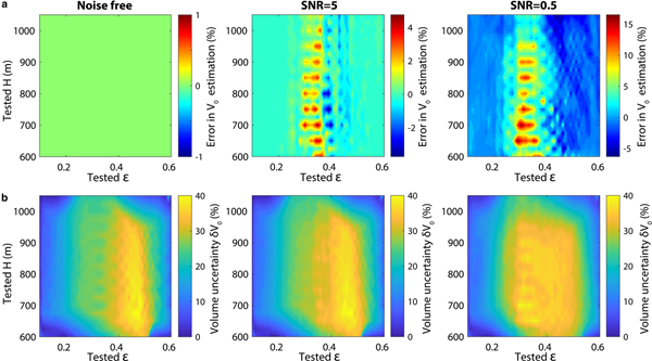

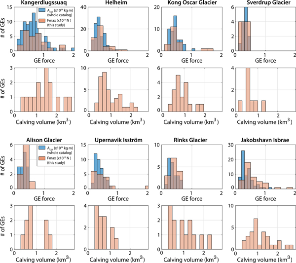


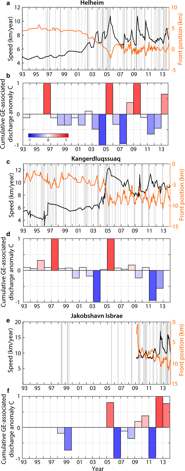


 Open access