


1. Introduction
A twin hull is the most common design of high-speed semi-displaced vessels, such as catamarans, air cushion vessels and skeg-type hovercraft, in which skegs can also serve as demihulls (Faltinsen Reference Faltinsen2005). A significant interest in the development of these types of vessels has arisen in the last decades due to the need for fast sea transportation of passengers and goods and for military applications. The advantages of twin hull vessels are mainly due to a large deck area, favourable stability characteristics, seakeeping and relative fuel saving. At the same time, twin hull vessels may experience slamming loads larger than conventional monohulls due to their smaller draft and the slamming of the bridge, or the deck referred to in the literature as ‘wetdeck slamming’.
A comprehensive review on ship slamming and impact load evaluation was recently provided by Dias & Ghidaglia (Reference Dias and Ghidaglia2018). Following Lafeber, Brosset & Bogaert (Reference Lafeber, Brosset and Bogaert2012), they explained the water impact of a steep wave as a combination of elementary loading processes consisting of the direct impact of the wave crest, the main liquid body impact with capturing of a gas bubble and the compression/expansion stage due to the bubble oscillations. Based on experimental observations, they concluded that the largest impact loading is associated with a rapid change of the total momentum of the liquid, which can be accounted for using the pressure impulse concept (Cooker & Peregrine Reference Cooker and Peregrine1995).
The pressure impulse concept has a long history, which goes back to the work of Lagrange (Reference Lagrange1781) and Havelock (Reference Havelock1927). A remarkable advancement in the impulse impact theory was made by von Kármán (Reference von Kármán1929) with application to seaplane landing. For ship slamming applications, Wagner (Reference Wagner1932), in his foundational paper, accounted for the rise of the free surface using the von Kármán solution. This approach received further development for solving modern water impact problems (Howison, Ockendon & Oliver Reference Howison, Ockendon and Oliver2004). There is also a large body of research dealing with the impulse impact concept, which includes the impulsive motion of a body initially floating on a flat free surface (Iafrati & Korobkin Reference Iafrati and Korobkin2005), dam-break flows (Korobkin & Yilmaz Reference Korobkin and Yilmaz2009), ice breaking by a high-speed water jet impact (Yuan et al. Reference Yuan, Ni, Wu, Xue and Han2022) and bubble collapse (Zhang et al. Reference Zhang, Li, Cui, Li and Liu2023).
According to this concept, the pressure at the time of impact tends to infinity, but the impact lasts an infinitesimal period of time. Recently, Speirs et al. (Reference Speirs, Langley, Pan, Truscott and Thoroddsen2021) investigated the impulsive impact of a flat bottom cylinder experimentally, accounting for the small compressibility of water. Not only did they find high pressures similar to previous studies, but they also revealed a decrease in the local pressure sufficient to cavitate the liquid. This occurs due to the pressure wave reflecting from the free surface and forming a negative pressure region. Thus, the pressure impulse concept is applicable to the determination of pressure loads for an impact duration small enough to neglect the motion of free surfaces but large enough to neglect the water compressibility.
All the studies mentioned above consider a single body floating on a free surface. By contrast, our research examines two bodies with a gap between them, which are synchronously set in motion. This case directly corresponds to the slamming of various vessels with twin hulls, such as catamarans. Another relevant case corresponds to ships containing a ‘moonpool’, i.e. vertical openings through the deck and the hull used for marine and offshore operations, such as pipe laying or diver recovery (Molin Reference Molin2001; Faltinsen, Rognebakke & Timokha Reference Faltinsen, Rognebakke and Timokha2007).
Mathematical models of impulse flows are based on the theory for an incompressible and irrotational flow, so that a velocity potential can be introduced. The free surface is assumed to be flat before the impact and the potential on the free surface remains zero during the impact. The boundary-value problem for the velocity potential can be written as follows:
 \begin{equation} \triangle \varPhi^\prime=0 , \end{equation}
in the fluid domain;
 \begin{equation} \varPhi^\prime=0 \end{equation}
on the free surface;
 \begin{equation} \frac{\partial \varPhi^\prime}{\partial n}=-Un_y , \end{equation}
on each body surface, where  $U$ is the velocity immediately after the impact, $\boldsymbol {n}$ is the outward normal to the body surface and $n_y$ is its component in the $y$ direction;
 \begin{equation} |\boldsymbol{\nabla}\varPhi^\prime |\rightarrow 0, \quad x^2+y^2 \rightarrow \infty, \end{equation}
which is the far-field condition.
Our solution method is based on a further extension of the integral hodograph method for solving two-dimensional boundary-value problems with mixed boundary conditions: there are two parts of the flow boundary with free surfaces and two parts corresponding to the two solid bodies where the impermeability condition is implied. The key step of the method is finding the two governing functions: the complex velocity and the derivative of the complex potential, both defined in an auxiliary parameter region. For the determination of the complex velocity, we derived an integral formula for solving a mixed boundary-value problem for an analytical function defined in a rectangular auxiliary parameter region. This formula makes it easy to determine an analytical function from the values of its argument given on the two horizontal sides of the rectangle corresponding to the solid bodies, and its modulus given on the two vertical sides corresponding to the two parts of the free surface.
The system of integral equations in the velocity angle along the body and the velocity magnitude along the free surface was derived by employing kinematic boundary conditions on the body and the free surface. These integral equations were solved numerically to complete the solution.
The coefficients of the added masses, the pressure impulse acting on the bodies and the velocity on the free surface including the gap between the bodies were determined for various widths of the gap and for various cross-sectional shapes of the impacting bodies, such as flat plates and half-circles.
2. Boundary-value problem
A sketch of the physical domain is shown in figure 1(a). Two bodies partially submerged in a liquid and connected by a deck float on the free surface. In general, the level of the liquid in the gap between the bodies may be different from the calm water level at infinity if the pressure in the gap chamber is different from the ambient pressure. The shapes of the bodies can be different; therefore, the chosen characteristic length  $L$ corresponds to the size of one of them. Before the time of impact, $t = 0$, the body and the liquid are at rest. At time $t = 0+$ the body is suddenly set in motion with acceleration $a$ directed downwards so that, during an infinitesimal time interval $\Delta t>0$, the velocity of the body reaches the value $U=a\Delta t$.
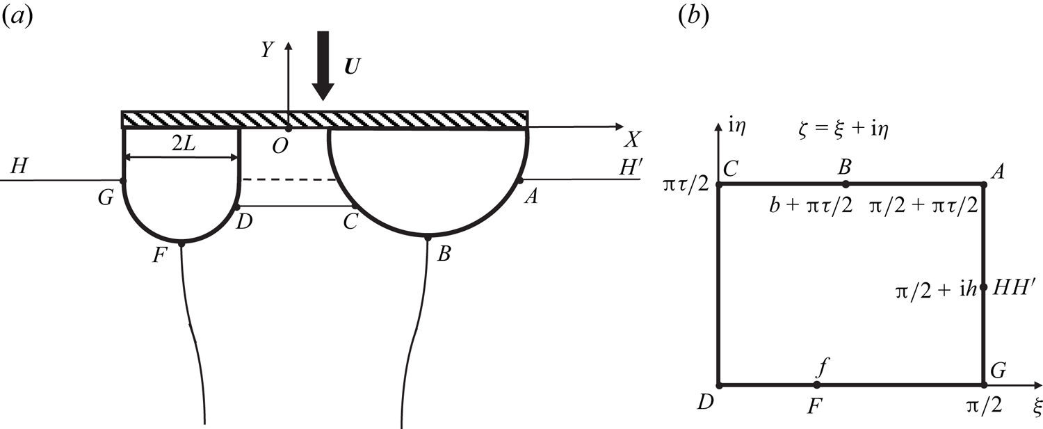
Figure 1. (a) Definition sketch of the physical domain and (b) the parameter, or  $\zeta$-plane.
The problem of a rigid body moving in a fluid body is kinematically equivalent to the problem of a fluid body moving around a fixed rigid body with acceleration  $a$ at infinity. We define a Cartesian coordinate system $XY$ attached to the deck, as shown in figure 1(a), and a coordinate system $X^\prime Y^\prime$, which coincides with $XY$ but attached to the calm free surface before the impact. Each body is assumed to have an arbitrary shape, which is defined by the slope of the body boundary, $\delta _i=\delta _i(S_{bi})$, as a function of the arc length coordinate $S_{bi}$ along the body $i$,
$i$,  $i=1,2$. The liquid is assumed to be ideal and incompressible, and the flow is irrotational. Gravity and surface tension effects during the impact are ignored. The contact points between the free surface and the body, $A$,
$A$,  $C$,
$C$,  $D$ and $G$, are shown in figure 1(a), as well as the stagnation points $B$ and $F$. The points $H$ and $H^\prime$ denote points of infinity on the free surface.
We introduce complex potentials  $W(Z)=\varPhi (X,Y)+{\rm i}\varPsi (X,Y)$ and $W^\prime (Z)= \varPhi ^\prime (X,Y)+{\rm i}\varPsi ^\prime (X,Y)$, with $Z=X+{\rm i}Y$ in the coordinate systems $XY$ and $X^\prime Y^\prime$, respectively. By integrating Bernoulli's equation over an infinitesimal time interval $\Delta t \rightarrow 0$ in each system of coordinates, we can obtain the relation between the pressure impulses in these systems of coordinates (Semenov, Savchenko & Savchenko Reference Semenov, Savchenko and Savchenko2021)
 \begin{equation} \varPi^\prime=\int_0^{\Delta t}p^\prime \,{\rm d}t=-\rho\varPhi^\prime=\varPi + \rho UY=-\rho\varPhi + \rho UY. \end{equation}
Here,  $\varPi$ and $\varPi ^\prime$ are the pressure impulses in the systems $XY$ and $X^\prime Y^\prime$, respectively; $p^\prime$ is the hydrodynamic pressure and $\rho$ is the density of the liquid.
The added mass coefficients,  $\lambda _{22}^{\prime }$ and $\lambda _{21}^{\prime }$, for the body $A^1$ (contour $DFG$) and body $A^2$ (contour $ABC$) of the bodies can be expressed as follows (Korotkin Reference Korotkin2009):
 \begin{equation} \lambda_{21}^{\prime1,2} =-\int_{s_D, s_A}^{s_G, s_C}\phi^\prime(s) \sin[\delta_{1,2}(s)]\,{\rm d}s, \quad \lambda_{22}^{\prime1,2} =-\int_{s_D, s_A}^{s_G, s_C}\phi^\prime \cos[\delta_{1,2}(s)]\,{\rm d}s. \end{equation}
Here,  $\phi (s) = \varPhi (S)/(LU)$ is the dimensionless potential normalized to $U$ and $L$;
$L$;  $s_A$, $s_C$, $s_D$, $s_G$ are the arc length coordinates of points $A$,
$A$,  $C$,
$C$,  $D$,
$D$,  $G$;
$G$;  $x = X/L$, $y = Y/L$, $s = S/L$; the dimensionless velocity on the free surface is $v = |V|/U$.
By substituting (2.1) in the dimensionless form into (2.2a,b) we obtain the relation between the added mass coefficients in the systems of coordinates  $X^\prime Y^\prime$ and $XY$
$XY$
 \begin{equation} \lambda_{21}^{\prime1,2} = \lambda_{21}^{1,2}, \quad \lambda_{22}^{\prime1,2} = \lambda_{22}^{1,2} - a^{{\ast} 1,2}, \quad a^{{\ast} 1,2} = \int_{s_D, s_A}^{s_G, s_C}y(s)\sin[\delta_{1,2}(s)]\,{\rm d}s. \end{equation}
 The coefficient  $\lambda _{22}^{1,2}$ accounts for the acceleration of the liquid in the $y$ direction during the impact, which is similar to gravity and causes the buoyancy force.
In the following, the objective is to determine the velocity potential of the flow  $\phi (s)$ in the system of coordinates $XY$, in which the liquid suddenly starts to move upward with velocity $U$.
$U$.
3. Conformal mapping
We choose the rectangle  $DGAC$ in the $\zeta$-plane with the vertices $(0,0)$, $({\rm \pi} /2,0)$, $({\rm \pi} /2,{\rm \pi} \tau /2)$ and $(0,{\rm \pi} \tau /2)$, respectively (figure 1b), as an auxiliary parameter region. Here, $\tau$ is an imaginary number. The horizontal length of the rectangle is equal to ${\rm \pi} /2$, and its vertical length is equal to ${\rm \pi} |\tau |/2$. The corresponding points of the rectangle and the flow region are denoted by the same letters. The horizontal sides of the rectangle $DG$ and $AC$ correspond to the surface of bodies $A^1$ and $A^2$, respectively. The vertical side $GA$ of the rectangle ( $\xi ={\rm \pi} /2, 0<\eta <{\rm \pi} /2$) corresponds to the free surface outside the twin body, i.e. $HG$
$HG$  $(0\leq \eta <{\rm i}h)$ and $AH^\prime$ $(h<\eta \leq {\rm \pi}/2)$. The vertical side $DC$ ( $\xi =0$, $0\leq \eta \leq {\rm \pi}/2$) corresponds to the free surface between the bodies. The positions of the stagnation points $F$ (
$F$ ( $\zeta =f$) and $B$ (
$B$ ( $\zeta =b+{\rm \pi} \tau /2$), and point $HH^\prime$ ( $\zeta ={\rm \pi} /2+{\rm i}h$) corresponding to infinity, have to be determined from the solution of the problem and physical considerations.
We formulate boundary-value problems for the complex velocity function,  ${\rm d}w/{\rm d}z$, and for the derivative of the complex potential, ${\rm d}w/{\rm d}\zeta$, both defined in the $\zeta$-plane. If these functions are known, then the derivative of the mapping function can be obtained (Joukovskii Reference Joukovskii1890; Michell Reference Michell1890)
 \begin{equation} \frac{{\rm d}z_m}{{\rm d}\zeta} = \left.\frac{{\rm d}w}{{\rm d}\zeta}\right/\frac{{\rm d}w}{{\rm d}z}, \end{equation}
and its integration in the  $\zeta$-plane gives the mapping function $z = z_m(\zeta )$ relating the coordinates in the parameter and the physical planes.
If a complex function is defined in a rectangle, it can be extended periodically onto the whole complex  $\zeta$-plane using the symmetry principle (Milne-Thompson Reference Milne-Thompson1962; Gurevich Reference Gurevich1965). This periodic domain is consistent with the definition domain of doubly periodic elliptic functions with periods ${\rm \pi}$ and ${\rm \pi} \tau$ along the $\xi$ and the $\eta$ axes, respectively. The derivation of the complex velocity (A4) and the derivative of the complex potential (A5) using Jacobi's theta functions is included in Appendix A. These equations include the parameters $b$,
$b$,  $f$,
$f$,  $h$,
$h$,  $K$,
$K$,  $\tau$, $c_1$, $c_2$ and $c_3$ and the functions $v_i(\eta )$, $\delta _i(\xi )$, $i=1,2$, all to be determined from physical considerations and the kinematic boundary condition on the free surface and the solid boundary of each body.
3.1. System of equations in the unknowns  $b$, $f$, $h$, $K$, $\tau$, $c_1$, $c_2$ and $c_3$


The constants  $c_1$, $c_2$ and $c_3$ are determined from the following conditions: the conjugate velocity direction at contact point $A$ (
$A$ ( $\zeta _A={\rm \pi} /2+{\rm \pi} \tau /2$), $\arg ({\rm d}w/{\rm d}z)_{(\zeta =\zeta _A)}=-\delta _A$; the velocity magnitude at infinity, point $H$ (
$H$ ( $\zeta _H = {\rm \pi}/2+{\rm i}h$) is assumed to be equal to unity, or $|{\rm d}w/{\rm d}z|_{(\zeta =\zeta _H)}=1$; the conjugate velocity direction at contact point $G$ (
$G$ ( $\zeta _G={\rm \pi} /2$) $\arg ({\rm d}w/{\rm d}z)_{(\zeta =\zeta _G)}=-\delta _G$.
For the determination of the unknowns  $b$,
$b$,  $f$,
$f$,  $h$,
$h$,  $K$ and $\tau$ we use the following conditions: the pressure impulse must be zero at contact points $D$ and $G$, or
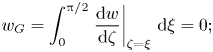 \begin{equation} w_G=\int_0^{{\rm \pi}/2}\left. \frac{{\rm d}w}{{\rm d}\zeta}\right|_{\zeta=\xi}\,{\rm d}\xi=0; \end{equation}
the wetted length of the first (second) body is  $S_{w1}(S_{w2})$
 \begin{equation} \int_0^{{\rm \pi}/2}\left|\frac{{\rm d}z_m}{{\rm d}\zeta}\right|_{\zeta=\xi({\xi+{{\rm \pi}\tau}/{2}})}\,{\rm d} \xi=S_{w1}\left({S_{w2}}\right)\!; \end{equation}
the level of the free surface at left and right infinities should be the same. Integrating the derivative of the mapping function (3.1) over an infinitesimal semi-circle centred at point  $H$ (
$H$ ( $\zeta _H={\rm \pi} /2+{\rm i}h$) will correspond to a contour of infinitely large radius in the physical plane with the ends belonging to the free surface. By evaluating the integral using residues and taking its imaginary part, we obtain
 \begin{equation} {\rm Im}\left(\oint_{\zeta=\zeta_H}\frac{{\rm d}z_m}{{\rm d}\zeta}{\rm d}\zeta \right)= {\rm Im}\bigg(\frac{{\rm i}{\rm \pi}}{-{\rm i}v_\infty} \begin{array}{c} ~~~ \\ \mbox{res}\\ ~^{\zeta=\zeta_H} \end{array} \frac{{\rm d}w}{{\rm d}\zeta} \bigg)= {\rm Im}\left\{ \frac{\rm \pi}{-v_\infty} \frac{{\rm d}}{{\rm d}\zeta } \left[\frac{{\rm d}w}{{\rm d}\zeta}(\zeta-\zeta_H)^2\right] \right\}=0. \end{equation}
By substituting the derivative of the complex potential (A5) into (3.4) and differentiating the expression in brackets, we reduce (3.4) to the following equation:
 \begin{align} {\rm Im}\left\{ \frac{\vartheta_1^\prime(\zeta_H-f)}{\vartheta_1(\zeta_H-f)} + \frac{\vartheta_1^\prime(\zeta_H+f)}{\vartheta_1(\zeta_H+f)} + \frac{\vartheta_4^\prime(\zeta_H-b)}{\vartheta_4(\zeta_H-b)} +\frac{\vartheta_4^\prime(\zeta_H+b)}{\vartheta_4(\zeta_H+b)} - 2\frac{\vartheta_2^\prime(\zeta_H+{\rm i}h)}{\vartheta_2(\zeta_H+{\rm i}h)}\right\}=0. \end{align}
 The distance between the bodies,  $S_{gap}$, is obtained by integrating the derivative of the mapping function along the vertical side $DC$ in the parameter plane
 \begin{equation} {\rm Re}\left(\int_0^{{{\rm \pi}|\tau|}/{2}} \left. \frac{{\rm d}z_m}{{\rm d}\zeta} \right|_{\zeta={\rm i}\eta}\right) {\rm d} \eta =S_{gap}. \end{equation}
3.2. Body boundary conditions for the function $\delta _i (\xi )$, $i=1,2$


By using the given functions  $\delta _i(s_{bi})$, $i=1,2$, where $s_{bi}$ is the arc length coordinate along the $i{\rm th}$ body, and changing the variables, we obtain the following integro-differential equations in the functions $\delta _i(\xi )$:
 \begin{equation} \frac{{\rm d}\delta_i}{{\rm d}\xi}=\frac{{\rm d}\delta_i}{{\rm d}s}\frac{{\rm d}s_{bi}}{{\rm d}\xi}= \frac{{\rm d}\delta_i}{{\rm d}s}\left|\frac{{\rm d}z_m}{{\rm d}\zeta}\right|_{\zeta=\xi}, \quad 0 \leq \xi \leq {\rm \pi}/2, \quad i=1,2, \end{equation}
where  $\zeta _1=\xi$ and $\zeta _2=\xi +{\rm \pi} \tau /2$ and the derivative of the mapping function (3.1) is used.
3.3. Free surface boundary conditions for the functions $v_i(\eta )$, i=1,2

An impulsive impact is characterized by an infinitesimally small time interval  $\Delta t \rightarrow 0$ such that the position of the free surface does not change during the impact. From the Euler equations it follows that the impact-generated velocity is perpendicular to the free surface (since the pressure is constant)
 \begin{equation} \arg \left( \left.\frac{{\rm d}w}{{\rm d}z}\right|_{\zeta=\bar{\zeta}_i} \right) =-\frac{\rm \pi}{2}, \quad i=1,2, \end{equation}
where  $\bar {\zeta }_1={\rm \pi} /2 +{\rm i}\eta$, $\bar {\zeta }_2={\rm i}\eta$, $0 \leq \eta \leq {\rm \pi}|\tau |/2$.
Taking the argument of the complex velocity from (A4), we obtain the following integral equation in the functions  ${\rm d}\ln v_i/{\rm d}\eta$, $i=1,2$:
 \begin{align} &\frac{(-1)^{i+1}}{\rm \pi}\int_0^{{{\rm \pi}|\tau|}/{2}}\frac{{\rm d}\ln v_i}{{\rm d}\eta^\prime} \ln\left|\frac{\vartheta_1(\eta-\eta^\prime)}{\vartheta_1(\eta+\eta^\prime)} \right|{\rm d} \eta^\prime\nonumber\\ &\quad =-\frac{\rm \pi}{2}-I_{bi}(\eta)-I_{vi}(\eta)-c_1\eta - c_3,\quad 0 \leq \eta \leq {\rm \pi}|\tau|/2, \quad i=1,2, \end{align}
where
 \begin{equation} \left.\begin{aligned} I_{bi}(\eta) & =\frac{1}{\rm \pi}\int_0^{{\rm \pi}/{2}}\frac{{\rm d}\delta_1}{{\rm d}\xi}{\rm Im} \left\{\ln \frac{\vartheta_{3-i}({\rm i}\eta-\xi)}{\vartheta_{3-i}({\rm i}\eta+\xi)} \right\} {\rm d}\xi \\ & \quad + \frac{1}{\rm \pi}\int_{{\rm \pi}/{2}}^0\frac{{\rm d}\delta_2}{{\rm d}\xi}{\rm Im} \left\{\ln \frac{\vartheta_{i+2}({\rm i}\eta-\xi)}{\vartheta_{i+2}({\rm i}\eta+\xi)} \right\}{\rm d}\xi,\\ I_{vi}(\eta) & = {\rm Im}\left\{\ln\frac{\vartheta_{3-i}({\rm i}\eta-f)\vartheta_{i+2}({\rm i}\eta-b)} {\vartheta_{3-i}({\rm i}\eta+f)\vartheta_{i+2}({\rm i}\eta+b)} \right\}\\ & \quad + \frac{(-1)^i}{\rm \pi}\int_0^{{{\rm \pi}|\tau|}/{2}}\frac{{\rm d}\ln v_{3-i}}{{\rm d}\eta^\prime}\ln\left|\frac{\vartheta_2({\rm i}\eta^\prime -\eta)}{\vartheta_2({\rm i}\eta^\prime +\eta)}\right|{\rm d}\eta^\prime. \end{aligned}\right\} \end{equation}
Equation (3.9) is a Fredholm integral equation of the first kind with a logarithmic kernel, which is solved numerically.
By using a small-time expansion, the first-order approximation of the free surface can be obtained as follows:
 \begin{equation} \bar{\eta}(x,t)=\bar{\eta}(x,0) + \frac{\partial \bar{\eta}}{\partial t}(x,0)t + \ldots. \end{equation}
Here, the kinematic boundary condition on the free surface (the velocity is perpendicular to the free surface) is used
 \begin{equation} \frac{\partial \bar{\eta}}{\partial t}[x(\eta),0]=-{\rm Im}\left( \frac{{\rm d}w}{{\rm d}z}\right)_{\zeta={\rm i}\eta} =v[x(\eta),0]. \end{equation}
3.4. Numerical approach
In discrete form, the solution is sought on a fixed set of nodes  $\zeta _j$, $j=1,\ldots, 5M$, distributed along the boundary of the rectangle $DGAC$. The numbering starts and ends at point $D$. Each part $DG$,
$DG$,  $GH$,
$GH$,  $HA$,
$HA$,  $AC$ and $CD$ of the boundary is discretized using $M$ points and the cosine law to provide a higher density of nodes $\zeta _j$ near points $D (\widehat {\zeta _0})$, $G (\widehat {\zeta _1})$, $H (\widehat {\zeta _2})$, $A (\widehat {\zeta _3})$ and $C (\widehat {\zeta _4})$ as follows:
 \begin{align} \zeta_j &=
\hat{\zeta}_{i-1} +(\widehat{\zeta_i} -
\hat{\zeta}_{i-1})*\left( 1-\cos\frac{j- (i-1)M}{M-1}
\right)\!, \notag\\ j&=(i-1)M+1,\ldots, iM, \quad i=1,5,
\end{align}
\begin{align} \zeta_j &=
\hat{\zeta}_{i-1} +(\widehat{\zeta_i} -
\hat{\zeta}_{i-1})*\left( 1-\cos\frac{j- (i-1)M}{M-1}
\right)\!, \notag\\ j&=(i-1)M+1,\ldots, iM, \quad i=1,5,
\end{align}
where  $\widehat {\zeta _0} = (0,0)$, $\widehat {\zeta _1} = ({\rm \pi} /2, 0)$, $\widehat {\zeta _2} = ({\rm \pi} /2, \textrm {i}h)$, $\widehat {\zeta _3} = ({\rm \pi} /2, {\rm \pi}\tau /2)$, $\widehat {\zeta _4} = (0, {\rm \pi}\tau /2)$, $\widehat {\zeta _5} = (0, 0)$. The number $M$ is chosen in the range from $M=50$ to $M=400$ based on the requirement to provide the convergence of the solution and its reasonable accuracy. The integrals appearing in (A4) are evaluated on the intervals ( $\zeta _{j-1},\zeta _j$) using a linear interpolation of the functions $\delta _{1,2}(\xi )$ and $\ln v_{1,2}(\eta )$, and the $8$-point Legendre–Gauss quadrature formula.
The system of nonlinear equations (3.9) is solved using the iteration Newton method, at each iteration of which the system of nonlinear equations (3.2), (3.3), (3.6) and the integro-differential equation (3.7) are solved by the method of successive approximations using nested iteration procedures. Several tens of iterations are necessary for solving (3.9) and (3.7) to get a converged solution with a tolerance less than  $10^{-6}$.
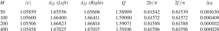
The accuracy of the calculations depends on the discretization of the horizontal and the vertical sides of the rectangle in the parameter plane. Table 1 shows the convergence of the added mass and other parameters as the number of discretization points  $M$ increases and the intervals $(\zeta _j, \zeta _{j-1})$ diminish, including the intervals closest to the contact points between the free surface and the plates, $D$,
$D$,  $C$,
$C$,  $G$ and $A$. This provides a more accurate evaluation of the integrals in (A4) because the functions $\ln v_{1,2}(\eta )$ are singular, but integrable at the contact points. It can be seen that the difference of the parameters between two adjacent lines in the table decreases as the number of discretization points $M$ doubles. The length of the intervals near points $C$ and $D$ (they are the same according to the distribution (3.13)) is shown in the rightmost column of the table.
Table 1. Convergence of the solution for various discetizations of the boundary of the parameter rectangle for the case  $Sgap/L=1$; $\Delta \eta =-\textrm {Im}(\zeta _{5M}-\zeta _{5M-1})$.
4. Results and discussion
Figure 2 shows streamline patterns (left axis) and the velocity magnitude on the free surface (right axis) for the impulsive impact of twin plates in the system of coordinates attached to the plate (a) and to the liquid at rest (b). As expected, the density of the streamlines is higher near the plate edges, which corresponds to a higher velocity. This agrees with the velocity magnitude on the free surface shown in the upper part of the figures. The magnitude of the velocity rapidly increases, tending to infinity at the edges. On the free surface between the plates, the velocity reaches its minimum at the middle of the gap (due to the flow symmetry), which is higher than the velocity at infinity since the plates push the liquid into the gap. The pressure impulse on the plate is shown as a blue curve. It is the same in both systems of coordinates (2.1) because the thickness of the plate is zero.
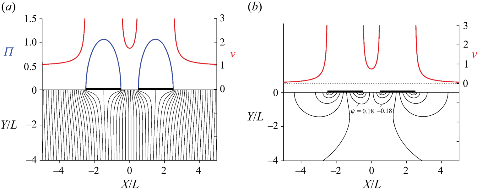
Figure 2. The streamline patterns (left axis), the velocity magnitude on the free surface (right axis, red curve) and the pressure impulse (left axis, blue curve) in the system of coordinates attached to the plate (a) and to the calm free surface before the impact (b). The length of each plate is  $2L$ and the gap $S_{gap}=L$.
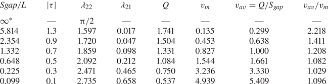
The main flow parameters are shown in table 2 for various widths of the gap: the added mass coefficient  $\lambda _{22}$; the discharge through the gap, $Q$; the minimal velocity in the gap, $v_m$; the average velocity in the gap, $v_{av}$; the ratio $v_{av}/v_m$; and the parameter $2b/{\rm \pi}$. Due to the flow symmetry the parameter $f=b$ and $h={\rm \pi} |\tau |/4$. As the gap tends to infinity, the flow near each plate becomes the same as for an isolated flat plate. As the gap tends to zero, the total length of the plates increases twice, $4L$, and the total added mass increases by a factor of $4$ (
$4$ ( $L^2$) and becomes $2{\rm \pi}$. It can be seen that the added mass of each plate approaches ${\rm \pi}$, or the total added mass of the two plates approaches $2{\rm \pi}$. As the gap gets smaller, the velocity in the gap increases due to the infinite velocity at the edges of the plate. This causes a moderate flow rate through the gap even for extremely small gaps. The ratio of the average velocity to the minimum velocity in the gap tends to the value which is close to ${\rm \pi} /2$.
Table 2. Main parameters of the impulsive impact of the twin plates; the number of nodes  $M=400$.
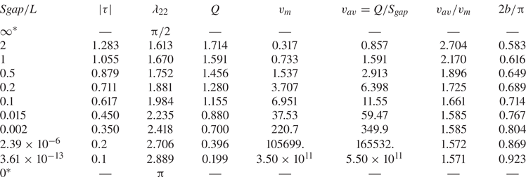
Figure 3 shows the results for twin half-circles of diameter  $2L$ each and the gap $S_{gap} = L$. The streamlines corresponding to the stagnation points in figure 3(a) are slightly inclined to each other so that the distance between them increases near the bodies. This means that the velocity there is smaller than at infinity, but then it rapidly increases in the gap near the free surface. The velocity on the free surface is finite everywhere, including the contact points of the free surface and the circles. This is because the slope of the circles at the contact points equals ${\rm \pi} /2$, which is the same as the velocity direction on the free surface, and therefore there is no jump in the velocity direction at the contact points and, correspondingly, there is no singularity in the function of the complex velocity at these points.
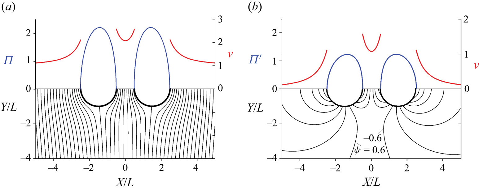
Figure 3. Same as in figure 2 but for two half-circles.
The streamlines corresponding to the impulsive motion of the twin half-circles are shown in figure 3(b) together with the velocity distribution on the free surface in the upper part of the figure. All the streamlines start on the circles, which move down with velocity  $U$, and end on the free surface, except for the two streamlines separating those ending on the free surface in the gap between the half-circles and on the rest of the free surface. The half-circles push the liquid into the gap, which results in a much higher velocity on the free surface in the gap than on the rest of the free surface.
For shaped bodies, the additional functions  $\delta _{1, 2}(\xi )$ are included into the computations. They are computed by a nested iteration procedure when solving the integro-differential equation (3.7). Both the functions $\delta _{1, 2}(\xi )$ and the function
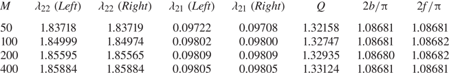
  $\ln v_{1, 2}(\eta )$ are non-singular. The convergence of the solution for the two circular cylinders is evident from table 3.
Table 3. Convergence of the solution for the twin cylinders in the case  $|\tau |=0.7$, $Sgap/L=1.332$.
The main flow parameters are shown in table 4 for various widths of the gap. Due to the identical geometry of the bodies, there is a line of flow symmetry,  $x=0$, which can be considered as a rigid wall, which results in a non-zero force acting on each body in the $x$-direction; therefore, the added mass coefficient $\lambda _{21}\neq 0$. As the gap decreases, the velocity on the free surface increases, but remains finite in contrast to the results corresponding to the flat plate. The ratio of the average velocity to the minimum velocity in the gap approaches unity; this means that the velocity distribution on the free surface in the gap becomes almost uniform.
Table 4. Main parameters of the impulsive impact of the twin half-circles; the number of nodes  $M=400$.
The impulsive impact of a non-symmetric twin body whose cross-section consists of a circle and the flat plate is shown in figure 4. As expected, the streamlines and the velocity magnitude on the free surface are no longer symmetric about the  $y$-axis. The remarkable feature is that the pressure impulse on the circle and the plate in figure 4(b) is almost the same. This sheds some light on why Wagner's theory based on the flat plate impulsive impact predicts well water impacts of blunt-shaped bodies. However, when the liquid impacts the twin body, the pressure impulse acting on the submerged cross-section is significantly larger than that acting on the plate, as can be seen in figure 4(a). The buoyancy force makes a significant contribution to the pressure impulse for the submerged cross-section.
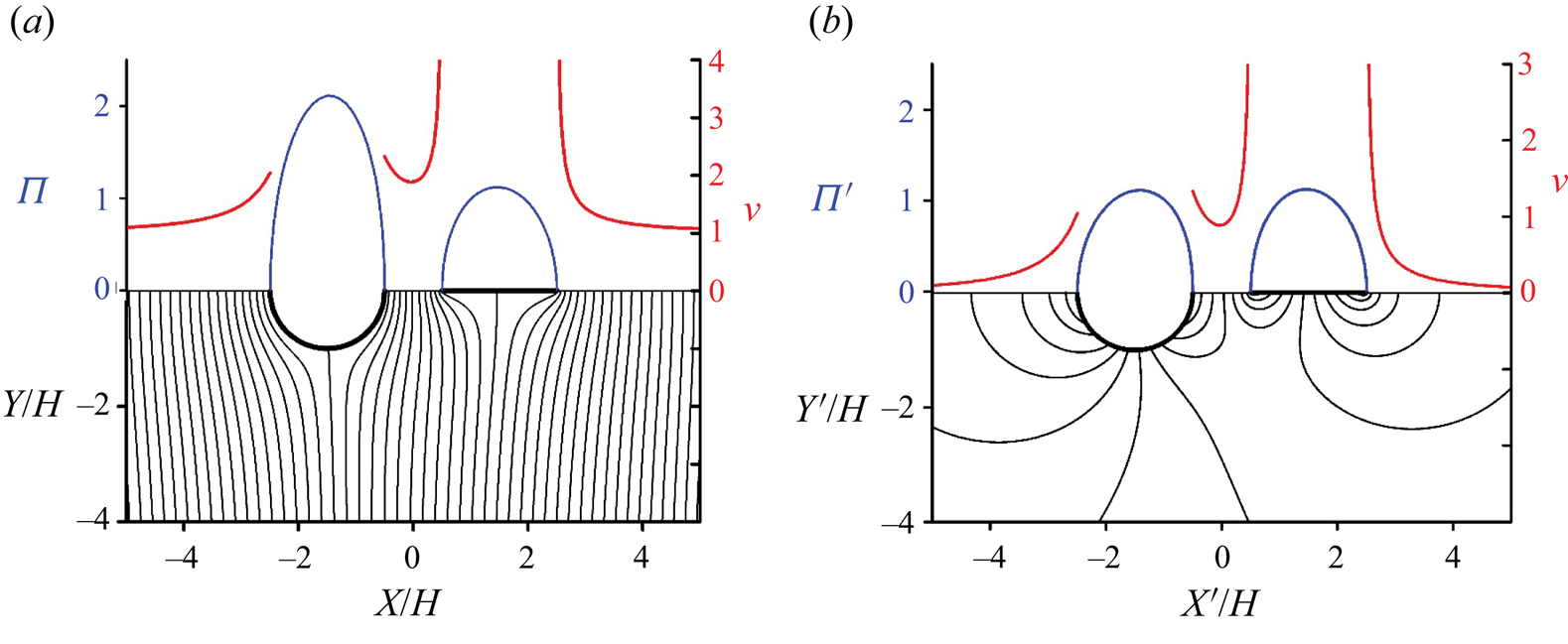
Figure 4. Same as in figure 2 but for circle and plate cross-sectional shapes.
The results in figure 4 were compared with the case of the twin body consisting of the flat plate (a) and the circle (b). As expected, the obtained results are a mirror reflection of those shown in figure 4.
5. Conclusions
An impulsively starting flow generated by a pair of bodies floating on a free surface is studied using the integral hodograph method. A rectangle is chosen as the parameter plane, and the solution is obtained in terms of Jacobi's quasi-doubly periodic theta functions. The boundary-value problem is reduced to a system of integral equations in the functions of the velocity direction on the solid boundaries and the velocity magnitude on the free surface, which is solved numerically.
The streamline patterns, the velocity distribution on the free surface and the pressure impulse along the bodies are presented for identical and different cross-sectional shapes of the bodies, such as plates and half-circles.
The main flow parameters are determined as a function of the width of the gap. It is shown that, as the gap tends to infinity, the flow parameters tend to their values corresponding to the impulsive impact of a single body; as the gap tends to zero, the flow parameters also tend to values corresponding to a single body but a larger dimension. The computations are analysed for different numbers of nodes on the boundary of the rectangle in the parameter plane, and the convergence of the solution is demonstrated. The results can be used as benchmark results when studying the problem using alternative approaches, although comparisons with experiments are desirable to better understand the extent to which the pressure impulse concept works well.
The obtained solution is also applicable to the study of an upward impact since the boundary conditions are the same but the velocity direction is the opposite. The obtained solution can be considered as a first-order solution in solving the problem using the method of small time series.
Chung (Reference Chung1977) conducted experiments on the determination of the added mass of two-dimensional submerged bodies. He determined the added masses as a function of the frequency of vertical oscillations and the depth of submergence of a beam with squared and circular cross-sections. His experiments supported the pressure impulse concept, but they are not applicable for comparisons in the present case. In order to determine the added masses of a floating twin body, the experimental set-up should be modified to avoid the effect of the waves generated during the vertical oscillatory motion of the floating body.
Acknowledgements
YAS would like to thank the Isaac Newton Institute for Mathematical Sciences and the London Mathematical Society for the financial support within the Solidarity Satellite Programme from July 2022 to January 2023 and the School of Mathematical Sciences UEA as host organization, when this work was started.
Funding
This work is supported by the National Natural Science Foundation of China (nos. 52192693, 52192690, 52371270 and U20A20327), and the National Key Research and Development Program of China (2021YFC2803400), to which the authors are most grateful.
Declaration of interests
The authors report no conflict of interests.
Appendix A. Expressions for the complex velocity and the derivative of the complex potential
The body is considered to be fixed; therefore, the velocity direction on each body is determined by the slope of the body,  $\delta _i=\delta _i(s_{bi})$, $i=1,2$. Besides, at this stage, we assume that the argument of the complex velocity $\chi _i(\xi )=-\textrm {d}\delta _i/\textrm {d}s [s_{bi}(\xi )]$ is a known function of the parameter variable $\xi$ and the velocity magnitude on each part of the free surface is a known function of the parameter variable $\eta$, or $v_i=v_i(\eta )$,
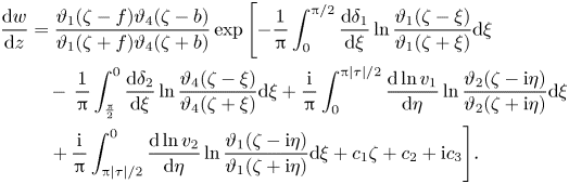
  $i=1,2$. To determine the complex velocity, we have to derive an integral formula that determines a complex function defined in a rectangular domain from its values on the horizontal and vertical sides of the rectangle. By applying the special point method (Gurevich Reference Gurevich1965) and proceeding similarly to Semenov & Wu (Reference Semenov and Wu2020), the following integral formula can be obtained:
 \begin{align} \frac{{\rm d}w}{{\rm d}z}&=\exp\left[-\frac{1}{\rm \pi}\int_0^{{\rm \pi}/2} \frac{{\rm d}\chi_1}{{\rm d}\xi}\ln\frac{\vartheta_1(\zeta-\xi)}{\vartheta_1(\zeta+\xi)} {\rm d}\xi -\frac{1}{\rm \pi}\int_{{\rm \pi}/2}^0\frac{{\rm d}\chi_2}{{\rm d}\xi}\ln\frac{\vartheta_4(\zeta-\xi)}{\vartheta_4 (\zeta+\xi)} {\rm d}\xi\right.\nonumber\\ &\quad +\frac{{\rm i}}{\rm \pi}\int_0^{{{\rm \pi}|\tau|}/{2}}\frac{{\rm d}\ln v_1}{{\rm d}\eta}\ln\frac{\vartheta_2(\zeta-{\rm i}\eta)}{\vartheta_2(\zeta+{\rm i}\eta)} {\rm d}\xi \nonumber\\ &\quad \left. +\,\frac{{\rm i}}{\rm \pi}\int_{{{\rm \pi}|\tau|}/{2}}^0 \frac{{\rm d}\ln v_2}{{\rm d}\eta}\ln\frac{\vartheta_1(\zeta-{\rm i}\eta)}{\vartheta_1(\zeta+{\rm i}\eta)} {\rm d}\xi + c_1\zeta + c_2 + {\rm i}c_3\right]\!, \end{align}
where  $\vartheta _i(\zeta )$, $i=1,2,4$ are Jacobi's doubly periodic theta functions, and $c_i$, $i=1,3$ are real constants to be determined from the conditions for the magnitude and direction of the velocity at infinity, $\zeta =\zeta _h={\rm \pi} /2+\textrm {i}h$ and the angle determining the orientation between the bodies. By substituting into (A1) $\zeta$ laying on the boundary of the rectangle, we can verify that the boundary conditions for the function dw/dz are satisfied
 \begin{align} \arg\left(\frac{{\rm d}w}{{\rm d}z}\right)_{\zeta=\xi \{\zeta=\xi+{{\rm \pi}\tau}/{2} \}}=\chi_1(\xi)\{\chi_2(\xi)\}, \quad \left|\frac{{\rm d}w}{{\rm d}z}\right|_{\zeta={\rm \pi}/{2}+{\rm i}\eta \{\zeta = {\rm i}\eta \}}=\frac{v_1(\eta)}{v_H} \left\{ \frac{v_2(\eta)}{v_C} \right\}\!, \end{align}
where  $v_H = v_1(\eta )_{\eta =h} = 1$ is the velocity at infinity, and $v_C=|\textrm {d}w/\textrm {d}z|_{\zeta ={\rm \pi} \tau /2}$ is the velocity at point $C$.
$C$.
The velocity direction at the stagnation points  $F$ and $B$ changes by ${\rm \pi}$; thus we can write
 \begin{equation} \chi_i (\xi ) = \arg \left(\frac{{\rm d}w}{{\rm d}z} \right) = \left\{\begin{array}{@{}ll} - \delta_i(\xi) + {\rm \pi}, & 0 \leq \xi \leq f, \eta = 0, \ i=1, \\ & b \leq \xi \leq {\rm \pi}/2, \ \eta = {\rm \pi}|\tau|/2, i=2, \\ - \delta_i(\xi) , & f \leq \xi \leq {\rm \pi}/2, \ \eta = 0, \ i=1, \\ & 0 \leq \xi \leq b, \ \eta = {\rm \pi}|\tau|/2, \ i=2. \end{array} \right. \end{equation}
 By substituting (A3) into (A1) and evaluating the integrals over the step change of the functions  $\chi _1(\xi )$ and $\chi _2(\xi )$ at points $F$ and $B$, we obtain the following expression for the complex velocity:
 \begin{align} \frac{{\rm d}w}{{\rm d}z}&= \frac{\vartheta_1(\zeta-f)\vartheta_4(\zeta-b)}{\vartheta_1(\zeta+f)\vartheta_4(\zeta+b)} \exp\left[-\frac{1}{\rm \pi}\int_0^{{\rm \pi}/{2}}\frac{{\rm d}\delta_1}{{\rm d}\xi}\ln\frac{\vartheta_1(\zeta-\xi)} {\vartheta_1(\zeta+\xi)} {\rm d}\xi\right.\nonumber\\ &\quad -\,\frac{1}{\rm \pi}\int_{\frac{\rm \pi}{2}}^0\frac{{\rm d}\delta_2}{{\rm d}\xi}\ln\frac{\vartheta_4(\zeta-\xi)}{ \vartheta_4(\zeta+\xi)}{\rm d}\xi +\frac{{\rm i}}{\rm \pi}\int_0^{{{\rm \pi}|\tau|}/{2}} \frac{{\rm d}\ln v_1}{{\rm d}\eta}\ln\frac{\vartheta_2(\zeta-{\rm i}\eta)}{\vartheta_2(\zeta+{\rm i}\eta)} {\rm d}\xi\nonumber\\ &\quad \left. +\, \frac{{\rm i}}{\rm \pi}\int_{{{\rm \pi}|\tau|}/{2}}^0 \frac{{\rm d}\ln v_2}{{\rm d}\eta}\ln\frac{\vartheta_1(\zeta-{\rm i}\eta)}{\vartheta_1(\zeta+{\rm i}\eta)} {\rm d}\xi + c_1\zeta + c_2 + {\rm i}c_3\right]\!. \end{align}
Here, we used the relation between the theta functions  $\vartheta _i(\zeta )$, $i=1,2,3,4$. The definition of the theta functions and their properties are shown in Appendix B.
We derive the derivative of the complex potential,  $\textrm {d}w/\textrm {d}\zeta$, using Chaplygin's singular point method (Gurevich Reference Gurevich1965, Chapter 1, § 5). The function $dw/d\zeta$ has simple zeros at the points $\zeta =f$ and $\zeta =b+{\rm \pi} \tau /2$ that correspond to the stagnation points $F$ and $B$ at which the streamline splits into two branches. At point $H$ (
$H$ ( $\zeta _H={\rm \pi} /2+\textrm {i}h$) the complex potential has a pole of the first order corresponding to a half-infinite flow domain (Gurevich Reference Gurevich1965, Chapter 1, § 5); therefore, the derivative of the complex potential at the point $\zeta _H$ has a pole of the second order. By extending the derivative of the complex potential symmetrically with respect to the sides $DG$ and $DC$ with the aim of providing real values of the complex potential on the vertical and horizontal sides of the rectangle, we have to put singularities of the same order in the symmetric points $\zeta =-f$, $\zeta =-b+{\rm \pi} \tau /2$ and $\zeta ={\rm \pi} /2-\textrm {i}h$. Then, using Liouville's theorem, the derivative of the complex potential can be written in the form
 \begin{equation} \frac{{\rm d}w}{{\rm d}\zeta}= K\frac{\vartheta_1(\zeta-f)\vartheta_1(\zeta+f)\vartheta_4(\zeta-b)\vartheta_4(\zeta+b)} {\vartheta_2^2(\zeta-{\rm i}h)\vartheta_2^2(\zeta+{\rm i}h)}, \end{equation}
where  $K$ is a real constant; the relations between the theta functions $\vartheta _i(\zeta )$, $i=1,2,3,4$ are shown in Appendix B.
Appendix B. Jacobi theta functions
Definition of four types of Jacobi theta functions and their properties (Whittaker & Watson Reference Whittaker and Watson1927)
 $$\begin{gather} \vartheta_1(\zeta)=2\sum_{n=1}^\infty(-1)^{n-1}q^{{1}/{4}(2n-1)^2}\sin(2n - 1)\zeta, \end{gather}$$
 $$\begin{gather}\vartheta_2(\zeta)=2\sum_{n=1}^\infty q^{{1}/{4}(2n-1)^2}\cos(2n - 1)\zeta, \end{gather}$$
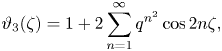 $$\begin{gather}\vartheta_3(\zeta)=1+2\sum_{n=1}^\infty q^{n^2}\cos2n\zeta, \end{gather}$$
 $$\begin{gather}\vartheta_4(\zeta)=1+2\sum_{n=1}^\infty(-1)^{n}q^{n^2}\cos2n\zeta, \end{gather}$$
where  $q = \textrm {e}^{{\rm \pi} \textrm {i}\tau }$. Theta functions can be expressed one through another as
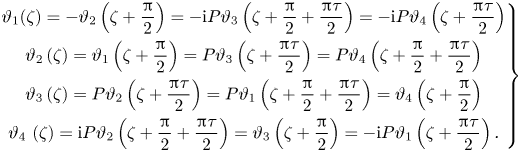 \begin{equation} \left.\begin{gathered} \vartheta_1(\zeta) =-\vartheta_2\left(\zeta+\frac{\rm \pi}{2}\right) =-{\rm i}P\vartheta_3 \left(\zeta+\frac{\rm \pi}{2}+\frac{{\rm \pi}\tau}{2}\right)=-{\rm i}P\vartheta_4\left(\zeta+\frac{{\rm \pi}\tau}{2}\right)\\ \vartheta_2\left(\zeta\right) = \vartheta_1\left(\zeta+\frac{\rm \pi}{2}\right) = P\vartheta_3\left(\zeta+\frac{{\rm \pi}\tau}{2}\right)= P\vartheta_4\left(\zeta+\frac{\rm \pi}{2}+ \frac{{\rm \pi}\tau}{2}\right) \\ \vartheta_3\left( \zeta \right) = P\vartheta_2\left(\zeta+\frac{{\rm \pi}\tau}{2}\right) = P\vartheta_1\left(\zeta+\frac{\rm \pi}{2}+\frac{{\rm \pi}\tau}{2}\right)= \vartheta_4\left(\zeta+\frac{\rm \pi}{2}\right) \\ \vartheta_4\ (\zeta) = {\rm i}P\vartheta_2\left(\zeta+\frac{\rm \pi}{2}+\frac{{\rm \pi}\tau}{2}\right) = \vartheta_3\left(\zeta+\frac{\rm \pi}{2} \right)=-{\rm i}P\vartheta_1\left(\zeta+\frac{{\rm \pi}\tau}{2}\right). \end{gathered}\right\} \end{equation}
Here,  $P = q^{-1/4} \textrm {e}^{\textrm {i}\zeta }$. The derivatives of the logarithm of the theta functions can be calculated using the fast converged series
 $$\begin{gather} \frac{\vartheta^\prime_1(\zeta)}{\vartheta_1(\zeta)} = \cot \zeta + 4\sum_{n=1}^\infty \frac{q^{2n} } {1-q^{2n}}\sin(2n\zeta), \end{gather}$$
 $$\begin{gather}\frac{\vartheta^\prime_2(\zeta)}{\vartheta_2(\zeta)} =-\tan \zeta + 4\sum_{n=1}^\infty(-1)^n\frac{ q^{2n}}{1-q^{2n}}\sin(2n\zeta). \end{gather}$$
 $$\begin{gather}\frac{\vartheta^\prime_3(\zeta)}{\vartheta_3(\zeta)} = 4\sum_{n=1}^\infty (-1)^n \frac{ q^n}{1-q^{2n}}\sin(2n\zeta) . \end{gather}$$
 $$\begin{gather}\frac{\vartheta^\prime_4(\zeta)}{\vartheta_4(\zeta)} = 4\sum_{n=1}^\infty \frac{ q^n}{1-q^{2n}}\sin(2n\zeta). \end{gather}$$


