


I. INTRODUCTION
Typical Internet of things (IoT) data collection environment using a base station with a large number of antennas in the 5th generation mobile communications systems (5G) [Reference Gupta and Jha1, Reference Andrews, Buzzi, Choi, Hanly, Lozano, Soong and Zhang2] can be considered as a special case of the massive multiuser multiple input multiple output (MU-MIMO) communications system. One of fundamental differences between the conventional massive MU-MIMO [Reference Saxena, Fijalkow and Swindlehurst3] and the IoT data collection is that the number of IoT nodes, in other words, the number of transmit antennas is typically much greater than that of receiving antennas even when a large antenna array is employed at the base station. Combined use with multiple access schemes will enable us to serve a large number of IoT nodes, but it also introduces additional delay, which may not be acceptable in many IoT applications.
MIMO systems having greater number of transmit antennas (more precisely, transmit streams) than that of receiving antennas is called overloaded MIMO [Reference Wong, Paulraj and Murch4–Reference Takahashi, Ibi and Sampei6]. The signal detection problem in such scenario is very difficult due to the underdetermined nature of the problem. However, if the transmit symbol takes discrete values on a finite set (alphabet) as in the case of digital communications, we can detect signals on the basis of maximum likelihood (ML) approach. Since the ML approach is not tractable in the case of massive overloaded MIMO detection, the signal detection method based on the local neighborhood search has been proposed [Reference Datta, Srinidhi, Chockalingam and Rajan7]. Moreover, since the computational complexity of the method is still too high when we use more than tens of transmit antennas, we have proposed a signal detection scheme using sum of absolute values (SOAV) optimization [Reference Hayakawa and Hayashi5], which is based on the idea of convex optimization and compressed sensing [Reference Donoho8, Reference Hayashi, Nagahara and Tanaka9]. This approach is especially effective when the number of antennas is large and the number of elements in the alphabet is small.
Taking advantage of the fact that the transmission rate from each IoT node is typically low, we have proposed a detection scheme for uplink orthogonal frequency division multiplexing (OFDM) IoT signals [Reference Hayashi, Nakai, Hayakawa and Ha10], where the overloaded MIMO signal reconstruction scheme in [Reference Hayakawa and Hayashi5, Reference Hayakawa and Hayashi11] is employed. However, the method cannot take the dependency between the real and the imaginary parts of the complex transmitted symbol into consideration because it is based on the SOAV optimization in the real-valued domain. In fact, it cannot use the fact that the real and the imaginary parts of the transmitted signal become $0$ simultaneously for non-active terminals. To tackle this problem, in [Reference Hayashi, Nakai-Kasai and Hayakawa12], we have employed a sparse complex discrete-valued vector reconstruction method named sum of complex sparse regularizers (SCSR) optimization [Reference Hayakawa and Hayashi13]. In [Reference Hayashi, Nakai-Kasai and Hayakawa12], we have focused on the overloaded MU-MIMO using single carrier block transmission with cyclic prefix (SC-CP) without precoding, which is equivalent to the MU-MIMO OFDM with precoding by a common discrete Fourier transform (DFT) matrix. In MU-MIMO SC-CP systems, neither the operations of inverse DFT (IDFT) nor the precoding is required at the transmitter, which can greatly reduce the complexity of IoT nodes. Moreover, the SC-CP signals have lower peak-to-average power ratio (PAPR) than the OFDM signals.
In this paper, we propose signal detection methods for uplink overloaded MU-MIMO systems on the basis of the preliminary conference papers [Reference Hayashi, Nakai, Hayakawa and Ha10, Reference Hayashi, Nakai-Kasai and Hayakawa12]. As mentioned above, the methods in [Reference Hayashi, Nakai, Hayakawa and Ha10, Reference Hayashi, Nakai-Kasai and Hayakawa12] use the discreteness of the transmitted signal vector to detect signals. However, since only a small number of terminals are typically active in the IoT transmission [Reference Liu, Larsson, Yu, Popovski, Stefanovic and de Carvalho14], the transmitted signal vector composed by concatenating transmitted signal vectors from all IoT nodes has not only the discreteness but also the group sparsity, i.e. most subvectors corresponding to the non-active terminals have all zero elements. To utilize such group sparsity, we propose discreteness and group sparsity aware (DGS) optimization, which uses two regularizers to promote both the discreteness and the group sparsity of the transmitted signal vector. The DGS optimization is a convex optimization problem in the complex-valued domain and hence it can also utilize the dependency between the real and the imaginary parts of the transmitted signals. We provide an optimization algorithm for the DGS optimization on the basis of the alternating direction method of multipliers (ADMM) [Reference Gabay and Mercier15–Reference Li, Wang and Wang19]. Moreover, we extend the DGS optimization into the weighted DGS (W-DGS) optimization so that we can use the prior information of the transmitted signal vector. We then propose an iterative approach called iterative weighted DGS (IW-DGS), where we iterate the W-DGS optimization and the parameter update in the objective function. We also discuss the computational complexity of the proposed IW-DGS. By using the structure of the channel matrix, we can reduce the order of the complexity. Simulation results show that the proposed IW-DGS can achieve good symbol error rate (SER) performance close to the oracle zero forcing (ZF) method, which perfectly knows the activity of each IoT terminal. We also show that the performance of the proposed method in MU-MIMO OFDM is significantly improved by using the precoding with the Hadamard matrix or the DFT matrix.
The additional contributions of this paper against the preliminary conference papers [Reference Hayashi, Nakai, Hayakawa and Ha10, Reference Hayashi, Nakai-Kasai and Hayakawa12] are summarized as follows.
• We newly propose the DGS optimization and the corresponding ADMM-based algorithm, which utilizes both the discreteness and the group sparsity of the transmitted signal vector. On the other hand, the method in the preliminary papers [Reference Hayashi, Nakai, Hayakawa and Ha10, Reference Hayashi, Nakai-Kasai and Hayakawa12] uses only the discreteness. In fact, the proposed DGS optimization can be considered as an extension of the SCSR optimization [Reference Hayakawa and Hayashi13] used in [Reference Hayashi, Nakai-Kasai and Hayakawa12]. Simulation results show that the performance is significantly improved by using the group sparsity.
• We also propose the iterative approach using the W-DGS optimization, which can achieve much better performance than the DGS optimization.
• We discuss the computational complexity of the proposed method, and show that we can reduce the order of the complexity by using the structure of the channel matrix.
• We demonstrate that the performance of the proposed method is comparable to the oracle ZF method, which perfectly knows the support of the transmitted signal vector, i.e. active IoT terminals, via computer simulations.
The rest of the paper is organized as follows. We describe the overloaded MU-MIMO OFDM system and the overloaded MU-MIMO SC-CP system in Section II. In Section III, we propose the overloaded signal detection methods. Section IV shows simulation results to demonstrate the performance of the proposed approach. Finally, Section V gives some conclusions.
We use the following notations in this paper. $\mathbb {R}$ is the set of all real numbers and $\mathbb {C}$
 is the set of all complex numbers. We denote the real part and the imaginary part by ${\rm Re}\{{\cdot }\}$
 and ${\rm Im}\{{\cdot }\}$
 , respectively. The transpose and the Hermitian transpose are indicated by $(\cdot )^{\mathsf {T}}$
 and $(\cdot )^{\mathsf {H}}$
 , respectively. We represent the imaginary unit by $j$
 , an $N \times N$
 identity matrix by $\boldsymbol {I}_{N}$
 , the $M \times N$
 zero matrix by $\textbf{0}_{M \times N}$
 , the $N \times 1$
 vector whose elements are all $1$
 by $\textbf{1}_{N}$
 , and the $N \times 1$
 vector whose elements are all $0$
 by $\textbf{0}_{N}$
 . For a vector $\boldsymbol {u}=\left [{u_{1}\, \ldots \, u_{N}}\right ]^{\mathsf {T}} \in \mathbb {C}^{N}$
 , we define the $\ell _{1}$
 and $\ell _{2}$
 norms of $\boldsymbol {u}$
 as $\left \lVert {\boldsymbol {u}}\right \rVert _{1} = \sum _{n=1}^{N} \left \lvert {u_{n}}\right \rvert$
 and $\left \lVert {\boldsymbol {u}}\right \rVert _{2} = \sqrt {\sum _{n=1}^{N} \left \lvert {u_{n}}\right \rvert ^{2}}$
 , respectively. ${\rm diag} (u_{1},\dotsc ,u_{N}) \in \mathbb {C}^{N \times N}$
 denotes the diagonal matrix whose $(n,n)$
 element is $u_{n}$
 . We represent the sign function by ${\rm sign}(\cdot )$
 . For a convex function $\phi : \mathbb {C}^{N} \to \mathbb {R} \cup \{\infty \}$
 , the proximity operator of $\phi$
 is defined as

II. SYSTEM MODEL
In this section, we describe the system model considered in this paper. In Table 1, we summarize the notation for the system model.
Table 1. Notation for the system model
A) Precoded MU-MIMO OFDM system
We consider uplink communications of IoT environments, which is modeled as a precoded MU-MIMO OFDM system. Figure 1 shows the system model, where the number of transmit terminals is $N$ , the number of receiving antennas at the base station is $M$
 , and the number of subcarriers is $Q$
 . Given that the number of transmit terminal is typically large in IoT environments, we focus on the overloaded scenario and assume $M<N$
 in this paper. The symbol alphabet and the frequency domain transmitted OFDM symbol vector from the $n$
 -th transmit IoT terminal are denoted by $\mathcal {S}$
 and $\boldsymbol {s}_{n}$
 , respectively. Here, taking IoT environment-specific feature into consideration, we assume only $N_{\text {act}}$
 IoT terminals out of $N$
 terminals are active meaning that only $N_{\text {act}}$
 terminals transmit OFDM signal blocks. Non-active $N-N_{\text {act}}$
 terminals actually keep silent, but we can regard they transmit all zero signal block $\textbf{0}_{Q}$
 . We thus have $\boldsymbol {s}_{n} \in \mathcal {S}^{Q}$
 when the $n$
 -th terminal is active, and otherwise $\boldsymbol {s}_{n}=\textbf{0}_{Q}$
 . When we use the cyclic prefix with the length greater than or equal to the channel order, the received signal vector after the removal of the cyclic prefix is given by

where $\boldsymbol {r}_{m}^{\text {f}, \text {OFDM}} \in \mathbb {C}^{Q}$ is the frequency domain received OFDM signal block at the $m$
 -th receiving antenna [Reference Hayashi, Nakai, Hayakawa and Ha10]. The diagonal matrix $\boldsymbol {\Lambda }^{(m,n)}={\rm diag} ({\lambda _{1}^{(m,n)},\dotsc ,\lambda _{Q}^{(m,n)}}) \in \mathbb {C}^{Q \times Q}$
 is composed of the channel frequency responses with the order of $L-1$
 between the $n$
 -th IoT terminal and the $m$
 -th receiving antenna. The diagonal elements can be written as

where $\boldsymbol {D} \in \mathbb {C}^{Q \times Q}$ is a $Q$
 -point unitary DFT matrix defined as

and $h_{1}^{(m,n)},\dotsc ,h_{L}^{(m,n)}$ denotes the impulse response of the frequency-selective channel between the $n$
 -th IoT terminal and $m$
 -th receiving antenna. $\boldsymbol {P} \in \mathbb {C}^{Q \times Q}$
 is a precoding matrix required to achieve good detection performance by the convex optimization-based detection scheme. Note that, in [Reference Hayashi, Nakai, Hayakawa and Ha10], we have numerically confirmed that we do not have to use different precoding matrices among IoT terminals, and a common Hadamard precoding matrix leads to good SER performance. $\boldsymbol {v}_{m}^{\text {f}} \in \mathbb {C}^{Q}$
 is the frequency domain additive white noise vector at the $m$
 -th receiving antenna with mean $\textbf{0}_{Q}$
 and covariance matrix $\sigma _{\text {v}}^{2}\boldsymbol {I}_{Q}$
 .
.
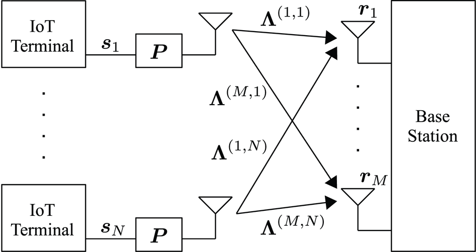
Fig. 1. Uplink MU-MIMO OFDM system for IoT environment.
B) Non-precoded MU-MIMO SC-CP system
Here, we show a non-precoded MU-MIMO SC-CP signal model. Assuming the length of cyclic prefix is greater than or equal to the channel order $L-1$ , the time domain received signal block at the $m$
 -th receiving antenna of the base station is written as

where $\boldsymbol {v}_{m}^{{\rm t}} \in \mathbb {C}^{Q}$ is the time domain additive white noise vector at the $m$
 -th receiving antenna having mean $\textbf{0}_{Q}$
 and covariance matrix $\sigma _{\text {v}}^{2} \boldsymbol {I}_{Q}$
 [Reference Hayashi, Nakai-Kasai and Hayakawa12, Reference Wang and Giannakis20]. By stacking from $\boldsymbol {r}_{1}^{\text {t}, \text {SC-CP}}$
 to $\boldsymbol {r}_{M}^{\text {t}, \text {SC-CP}}$
 in (4), and multiplying a unitary matrix of

from the left of both sides, we have the frequency domain received non-precoded SC-CP IoT signal vector at the base station as


where $\boldsymbol {r}_{m}^{\text {f}, \text {SC-CP}} \in \mathbb {C}^{Q}$ is the frequency domain received SC-CP signal vector at the $m$
 -th base station antenna and $\boldsymbol {v}_{m}^{\text {f}}=\boldsymbol {D}\boldsymbol {v}_{m}^{\text {t}}$
 ($m=1,\dotsc , M$
 ). It should be noted here that this received signal model can be regarded as a special case of (1), where the precoding matrix $\boldsymbol {P}$
 is set to be $\boldsymbol {D}$
 . Thus, if DFT matrix $\boldsymbol {D}$
 is appropriate for the precoding matrix of overloaded MU-MIMO OFDM system with the convex optimization-based signal detection, then the choice of non-precoded SC-CP signaling is extremely suited for IoT environments because this approach requires neither the IDFT operation nor the precoding operation at the IoT node (transmitter side).
III. PROPOSED SIGNAL DETECTION METHOD
The MU-MIMO OFDM signal model (1) and the MU-MIMO SC-CP signal model (7) can be represented as

Specifically, we have

in MU-MIMO OFDM systems and

in MU-MIMO SC-CP systems. $\boldsymbol {A}$ is the whole channel matrix given by

where $\boldsymbol {P}=\boldsymbol {D}$ in the case of MU-MIMO SC-CP. $\boldsymbol {s}=[{\boldsymbol {s}_{1}^{\mathsf {T}}\ \dotsb \ \boldsymbol {s}_{N}^{\mathsf {T}}}]^{\mathsf {T}} \in \mathbb {C}^{QN}$
 and $\boldsymbol {v}=\left [{\left ({\boldsymbol {v}_{1}^{\text {f}}}\right )^{\mathsf {T}}\ \dotsb \ \left ({\boldsymbol {v}_{M}^{\text {f}}}\right )^{\mathsf {T}}}\right ]^{\mathsf {T}} \in \mathbb {C}^{QM}$
 are the transmit symbol vector and the additive noise vector, respectively.
In this section, we describe the proposed signal detection method to estimate the transmitted symbol vector $\boldsymbol {s}$ from the received signal vector $\boldsymbol {r}$
 and the channel matrix $\boldsymbol {A}$
 in (8).
A) Discreteness and group sparsity of transmitted symbol vector
One of the main ideas of the proposed method is based on the fact that the transmitted symbol has the discreteness, i.e. the element of $\boldsymbol {s}$ is in the finite set $\mathcal {S} \cup \{ 0 \}$
 . For the reconstruction of such discrete-valued vector, several methods have been proposed [Reference Tan, Rasmussen and Lim21–Reference Nagahara24]. These methods reconstruct the discrete-valued vector in the real domain. For the reconstruction of the complex discrete-valued vector, SCSR optimization [Reference Hayakawa and Hayashi13] has been proposed by extending the approach in [Reference Nagahara24]. For details of the related methods, see Section III-F.
When only a few transmit terminals are active, the transmitted symbol vector $\boldsymbol {s}$ has not only the discreteness but also the group sparsity, i.e. $\boldsymbol {s}_{n}=\textbf{0}_{Q}$
 holds for most transmit terminals, because the transmitted symbol vector of non-active terminals can be regarded as $\textbf{0}_{Q}$
 . Note that not only is $\boldsymbol {s}$
 sparse, but multiple transmitted symbols from the non-active IoT terminal become zero simultaneously when OFDM or SC-CP signaling is employed. Such group sparsity has been utilized as prior knowledge in the literature of compressed sensing and sparse regression [Reference Yuan and Lin25–Reference Stojnic, Parvaresh and Hassibi27] as well as wireless communications [Reference Messai, Amis, Guilloud and Aïssa-El-Bey28, Reference Messai, Aïssa-El-Bey, Amis and Guilloud29]. Thus, we can expect a certain improvement of the detection performance by using the group sparsity of the transmitted signal vector $\boldsymbol {s}$
 .
.
B) Proposed DGS optimization
The proposed method utilizes both the discreteness and the group sparsity of $\boldsymbol {s}$ discussed in the previous subsection. The proposed DGS optimization problem is given by

where $c_{1},\dotsc ,c_{S}$ denotes all elements in $\{0\} \cup \mathcal {S}$
 . For example, when we use quadrature phase shift keying (QPSK) and set $\mathcal {S}=\left \{{1+j, -1+j, -1-j, 1-j}\right \}$
 , we have $S=5$
 and $c_{1}=0, c_{2}=1+j, c_{3}=-1+j, c_{4}=-1-j, c_{5}=1-j$
 . The vector $\boldsymbol {x}_{n} \in \mathbb {C}^{Q}$
 is the $n$
 -th subvector of $\boldsymbol {x}=\left [{\boldsymbol {x}_{1}^{\mathsf {T}}\ \dotsb \ \boldsymbol {x}_{N}^{\mathsf {T}}}\right ]^{\mathsf {T}} \in \mathbb {C}^{QN}$
 . $q_{\ell }$
 ($>0$
($>0$ ), $\alpha$
 ($>0$
($>0$ ), and $\varepsilon$
 ($>0$
($>0$ ) are parameters ($\ell =1,\dotsc ,S$
 ), where $\sum _{\ell =1}^{S}q_{\ell }=1$
 . The function $g_{\ell }(\cdot )$
 is a sparse regularizer for a sparse vector in the complex-valued domain. In this paper, we consider two convex regularizers given by


in accordance with [Reference Hayakawa and Hayashi13]. The first one $h_{1}(\cdot )$ is based on the modulus of the complex number, whereas the second one $h_{2}(\cdot )$
 considers the real part and the imaginary part separately. We can also use some non-convex sparse regularizers as in [Reference Hayakawa and Hayashi30], though the global optimizer cannot be necessarily obtained.
The objective function of the DGS optimization (12) is the weighted sum of two regularizers. The first term $\sum _{\ell =1}^{S} q_{\ell } g_{\ell } \left ({\boldsymbol {x} - c_{\ell }\textbf{1}}\right )$ in (12) has been proposed in [Reference Hayakawa and Hayashi13] as a regularizer for the discrete-valued vector. On the basis of the idea of compressed sensing [Reference Donoho8, Reference Hayashi, Nagahara and Tanaka9], the sparse regularizer $g_{\ell }(\cdot )$
 is applied by using the fact that $\boldsymbol {s}-c_{\ell }\textbf{1}$
 has some zero elements. A good choice of the sparse regularizer depends on the symbol alphabet $\mathcal {S}$
 . For example, when we use QPSK and set $c_{1}=0, c_{2}=1+j, c_{3}=-1+j, c_{4}=-1-j, c_{5}=1-j$
 , it is reasonable to define $g_{1}(\cdot )=h_{1}(\cdot )$
 and $g_{\ell }(\cdot )=h_{2}(\cdot )$
 ($\ell =2,\dotsc ,5$
 ). For more detailed discussion, see [Reference Hayakawa and Hayashi13]. In addition to the first regularizer, we also use the regularizer $\alpha \sum _{n=1}^{N} \left \lVert {\boldsymbol {x}_{n}}\right \rVert _{2}$
 to promote the group sparsity of $\boldsymbol {s}$
 . Note that we use the $\ell _{2}$
 norm $\left \lVert {\boldsymbol {x}_{n}}\right \rVert _{2}=\sqrt {\sum _{i=1}^{Q} \left \lvert {x_{n,i}}\right \rvert ^{2}}$
 of the complex-valued vector $\boldsymbol {x}_{n} = \left [{x_{n,1}\ \dotsb \ x_{n,Q}}\right ]^{\mathsf {T}} \in \mathbb {C}^{Q}$
 , whereas the $\ell _{2}$
 norm of the real valued vector is commonly used in the literature [Reference Yuan and Lin25–Reference Stojnic, Parvaresh and Hassibi27].
It should be noted that the conventional method [Reference Hayashi, Nakai, Hayakawa and Ha10] considers an optimization problem in the real domain, whereas the DGS optimization problem (12) is the optimization in the complex domain $\mathbb {C}^{QN}$ . Such approach enables us to directly utilize the discrete nature of the transmitted symbols in the complex domain. Moreover, the DGS optimization can utilize the group sparsity of the transmitted symbol vector, which has not been used in the conventional methods.
C) Proposed algorithm for DGS optimization based on ADMM
We here propose an algorithm for the DGS optimization. Since the objective function of the DGS optimization problem (12) is not differentiable, simple gradient-based methods cannot be applied. However, we can derive an optimization algorithm for the DGS optimization (12) on the basis of ADMM [Reference Gabay and Mercier15–Reference Li, Wang and Wang19] by appropriate reformulation as shown below. We firstly rewrite the DGS optimization problem (12) with new variables $\boldsymbol {z}_{1}, \dotsc , \boldsymbol {z}_{S}, \boldsymbol {z}_{\text {GS}} \in \mathbb {C}^{QN}$ and $\boldsymbol {z}_{\text {B}} \in \mathbb {C}^{QM}$
 as
as

In (17), we express the constraint $\left \lVert { \boldsymbol {r}-\boldsymbol {A}\boldsymbol {x} }\right \rVert _{2} \le \varepsilon$ in (12) by $\chi _{\mathcal {B}} \left ({\boldsymbol {z}_{\text {B}}}\right ) = \chi _{\mathcal {B}} \left ({\boldsymbol {A} \boldsymbol {x}}\right )$
 in the objective function, where we define $\mathcal {B} := \left \{{ \boldsymbol {u} \in \mathbb {C}^{QM} \,\left |\, \left \lVert {\boldsymbol {r}-\boldsymbol {u}}\right \rVert _{2} \le \varepsilon \right . }\right \}$
 and the corresponding indicator function

Since the objective function in (17) becomes infinity when $\boldsymbol {x}$ does not satisfy the constraint $\left \lVert { \boldsymbol {r}-\boldsymbol {A}\boldsymbol {x} }\right \rVert _{2} \le \varepsilon$
 , the optimization problem (17) is equivalent to the original optimization problem (12). The vector $\boldsymbol {z}_{\text {GS},n} \in \mathbb {C}^{Q}$
 is the $n$
 -th subvector of $\boldsymbol {z}_{\text {GS}}=[{\boldsymbol {z}_{\text {GS},1}^{\mathsf {T}}\ \dotsb \ \boldsymbol {z}_{\text {GS},N}^{\mathsf {T}}}]^{\mathsf {T}} \in \mathbb {C}^{QN}$
 . To further rewrite the optimization problem (17), we denote the objective function as


The constraint in (17) can also be summarized as $\boldsymbol {\Phi } \boldsymbol {x} = \boldsymbol {z}$ , where we define


By using the above expression, the DGS optimization problem (17) can be finally represented as

The optimization problem (23) is a standard form for ADMM, and hence we can derive the optimization algorithm based on ADMM.
The update equations of ADMM for (23) are given by


where $\rho$ ($>0$
($>0$ ) is a parameter and $\boldsymbol {w}^{k} \in \mathbb {C}^{(S+1)QN+QM}$
 . In the algorithm, $\boldsymbol {x}^{k}$
 is the estimate for the transmitted signal vector $\boldsymbol {s}$
 at the $k$
 -th iteration. The Wirtinger derivative [Reference Brandwood31] of $\left \lVert {\boldsymbol {\Phi }\boldsymbol {x}-\boldsymbol {z}^{k}+\boldsymbol {w}^{k}}\right \rVert _{2}^{2}$
 in (24) with respect to $\boldsymbol {x}$
 is given by

Here, in the same manner as $\boldsymbol {z}$ in (21), we define $\boldsymbol {w}_{1}^{k}, \dotsc , \boldsymbol {w}_{S}^{k}, \boldsymbol {w}_{\text {GS}}^{k} \in \mathbb {C}^{QN}$
 and $\boldsymbol {w}_{\text {B}}^{k} \in \mathbb {C}^{QM}$
 as the subvectors of the vector

From (28), $({\partial }/{\partial \boldsymbol {x}^{\mathsf {H}})} \{\left \lVert {\boldsymbol {\Phi }\boldsymbol {x}-\boldsymbol {z}^{k}+\boldsymbol {w}^{k}}\right \rVert _{2}^{2}\} = \textbf{0}$ gives the explicit formula for the update of $\boldsymbol {x}^{k}$
 in (24) as

The update of $\boldsymbol {y}^{k}$ in (25) can be expressed separately as

Next, we consider the update of $\boldsymbol {z}^{k}$ in (26), which can be denoted as


because the function $f(\cdot )$ is separable as in (20), where we have also used the property of proximity operator for translation [Reference Combettes and Pesquet17]. As discussed in [Reference Hayakawa and Hayashi13], the proximity operator of $\gamma g_{\ell }(\cdot )$
 can be computed by using


where $\gamma >0$ and $\boldsymbol {u} = [{u_{1}\ \dotsb \ u_{QN}}]^{\mathsf {T}} \in \mathbb {C}^{QN}$
 . We denote the $i$
 -th element of the vector by $[\cdot ]_{i}$
 . The proximity operator of $\gamma g_{\text {GS}}(\cdot )$
 is given by

where $\boldsymbol {u}_{n} \in \mathbb {C}^{Q}$ and $[{{\rm prox}_{\gamma g_{\text {GS}}} (\boldsymbol {u})}]_{n} \in \mathbb {C}^{Q}$
 are the $n$
 -th subvectors of $\boldsymbol {u}=\left [{\boldsymbol {u}_{1}^{\mathsf {T}}\ \dotsb \ \boldsymbol {u}_{N}^{\mathsf {T}}}\right ]^{\mathsf {T}} \in \mathbb {C}^{ QN}$
 and ${\rm prox}_{\gamma g_{\text {GS}}} (\boldsymbol {u})$
 , respectively. The proximity operator of $\gamma \chi _{\mathcal {B}}(\cdot )$
 can be written as the projection onto $\mathcal {B}$
 , i.e.

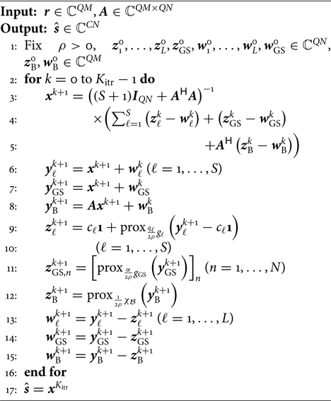
We summarize the proposed algorithm for the DGS optimization (23) in Algorithm 1.
Algorithm 1 Proposed Algorithm for DGS Optimization (23)
D) IW-DGS
By using the weighting technique in [Reference Hayakawa and Hayashi5, Reference Hayakawa and Hayashi13, Reference Candès, Wakin and Boyd32], we here extend the DGS optimization into the W-DGS optimization so that we can use prior information. Moreover, we propose an iterative approach named IW-DGS, where we iteratively solve the W-DGS optimization with the updated parameters.
Assuming that the sparse regularizer $g_{\ell }(\cdot )$ is separable as $h_{1}(\cdot )$
 or $h_{2}(\cdot )$
 , we extend the DGS optimization (12) to the W-DGS optimization given by

where $q_{i,\ell },\alpha _{n}$ ($>0$
($>0$ ) are the parameters. When $q_{i,\ell }=q_{\ell }$
 ($i=1,\dotsc ,QN$
 ) and $\alpha _{n}=\alpha$
 ($n=1,\dotsc ,N$
 ), the W-DGS optimization (38) is equivalent to the DGS optimization (12). In the W-DGS optimization (38), we can use the different coefficients $q_{i,\ell }$
 and $\alpha _{n}$
 for each transmitted symbol $s_{i}$
 and transmitted subvector $\boldsymbol {s}_{n}$
 , respectively. We can thus tune these parameters if we have some prior information about $\boldsymbol {s}$
 , e.g. a tentative estimate of $\boldsymbol {s}$
 .
.
We provide the ADMM-based algorithm for the W-DGS optimization (38). Letting $\tilde {g}_{\text {GS},n}(\boldsymbol {z}_{\text {GS}})=\lVert {\boldsymbol {z}_{\text {GS},n}}\rVert _{2}$ and $\tilde {f}(\boldsymbol {z})=\sum _{\ell =1}^{S} \sum _{i=1}^{QN} q_{i,\ell } g_{\ell } ({z_{i,\ell } - c_{\ell }}) + \sum _{n=1}^{N} \alpha _{n} \tilde {g}_{\text {GS},n}(\boldsymbol {z}_{\text {GS}}) + \chi _{\mathcal {B}} ({\boldsymbol {z}_{\text {B}}})$
 , we can rewrite the W-DGS optimization problem (38) as

where $\boldsymbol {z}=\left [{\boldsymbol {z}_{1}^{\mathsf {T}}\ \dotsb \ \boldsymbol {z}_{S}^{\mathsf {T}}\ \boldsymbol {z}_{\text {GS}}^{\mathsf {T}}\ \boldsymbol {z}_{\text {B}}^{\mathsf {T}}}\right ]^{\mathsf {T}} \in \mathbb {C}^{(S+1)QN+QM}$ , $\boldsymbol {z}_{\ell }=\break \left [{z_{1,\ell }\ \dotsb \ z_{QN,\ell }}\right ]^{\mathsf {T}} \in \mathbb {C}^{QN}$
 ($\ell =1,\dotsc ,S$
 ), and $\boldsymbol {z}_{\text {GS}}=[\boldsymbol {z}_{\text {GS},1}^{\mathsf {T}}\ \dotsb \break \boldsymbol {z}_{\text {GS},N}^{\mathsf {T}}]^{\mathsf {T}} \in \mathbb {C}^{QN}$
 . The ADMM-based algorithm for (39) can be obtained by replacing the update of $\boldsymbol {z}_{\ell }^{k}$
 and $\boldsymbol {z}_{\text {GS},n}^{k}$
 in Algorithm 1 with


respectively, where the vector $\boldsymbol {y}_{\text {GS},n}^{k+1} \in \mathbb {C}^{Q}$ is the $n$
 -th subvector of $\boldsymbol {y}_{\text {GS}}^{k+1}=[{{\boldsymbol {y}_{\text {GS},1}^{k+1}}^{\mathsf {T}}\ \dotsb \ {\boldsymbol {y}_{\text {GS},N}^{k+1}}]^{\mathsf {T}}}^{\mathsf {T}}$
 .
.
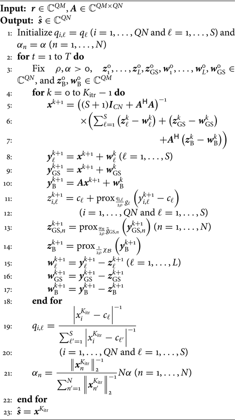
We propose an iterative algorithm named IW-DGS in Algorithm 2, where we iteratively compute the solution of the W-DGS optimization with the update of the parameters $q_{i,\ell }$ and $\alpha _{n}$
 .
.
Algorithm 2 IW-DGS
In Fig. 2, we show the illustration of the proposed IW-DGS. At each outer iteration $t$ , we update the parameters by using the tentative estimate at the previous iteration $t-1$
 . In this paper, we consider the update given by


where we define $\hat {\boldsymbol {s}}^{\text {pre}}=\left [{(\hat {\boldsymbol {s}}_{1}^{\text {pre}})^{\mathsf {T}}\ \dotsb \ (\hat {\boldsymbol {s}}_{N}^{\text {pre}})^{\mathsf {T}}}\right ]^{\mathsf {T}} =[\hat {s}_{1}^{\text {pre}}\ \dotsb \break \hat {s}_{QN}^{\text {pre}}]^{\mathsf {T}} \in \mathbb {C}^{QN}$ as the estimate of $\boldsymbol {s}$
 at the previous iteration. The denominators in (43) and (44) play the role of normalization to satisfy $\sum _{\ell =1}^{S} q_{i,\ell } = 1$
 for any $i=1,\dotsc ,QN$
 and $\sum _{n=1}^{N} \alpha _{n}=N\alpha$
 , respectively. By using (43) and (44), we can utilize the tentative estimate $\hat {\boldsymbol {s}}^{\text {pre}}$
 as the prior information. For example, the parameter $q_{i,\ell }$
 becomes large when the corresponding tentative estimate $\hat {s}_{i}^{\text {pre}}$
 is close to $c_{\ell }$
 . In this case, the new estimate of $s_{i}$
 also tends to be close to $c_{\ell }$
 . Similarly, the parameter $\alpha _{n}$
 becomes large when the norm of corresponding tentative estimate $\hat {\boldsymbol {s}}_{n}^{\text {pre}}$
 is small. In this case, the new estimate of $\boldsymbol {s}_{n}$
 also tends to become almost $\textbf{0}_{Q}$
 .
.
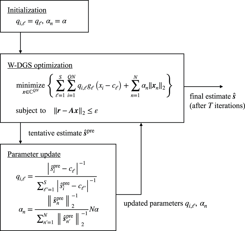
Fig. 2. Illustration of IW-DGS.
E) Computational complexity
We here discuss the computational complexity of IW-DGS in Algorithm 2. The order of the complexity is dominated by the computation of the inverse matrix $({(S+1) \boldsymbol {I}_{QN} + \boldsymbol {A}^{\mathsf {H}}\boldsymbol {A}})^{-1}$ , which requires $\mathcal {O}(Q^{3}N^{3})$
 complexity in a direct calculation [Reference Boyd and Vandenberghe33, Ch. 11]. However, by using the structure of $\boldsymbol {A}$
 , the order of the complexity can be reduced.
We firstly consider the computational complexity for $({(S+1) \boldsymbol {I}_{QN} + \boldsymbol {A}^{\mathsf {H}}\boldsymbol {A}})^{-1}$ in the case of MU-MIMO OFDM systems (11) without precoding, i.e. $\boldsymbol {P}=\boldsymbol {I}_{Q}$
 . In this case, $\boldsymbol {\Theta } := (S+1) \boldsymbol {I}_{QN} + \boldsymbol {A}^{\mathsf {H}}\boldsymbol {A} \in \mathbb {C}^{QN \times QN}$
 is composed of $N^{2}$
 diagonal matrices as

where $\boldsymbol {\Theta }^{(n_{1},n_{2})} = {\rm diag} ({\theta _{1}^{(n_{1},n_{2})}, \dotsc , \theta _{Q}^{(n_{1},n_{2})}}) = \delta _{n_{1}n_{2}}(S+1)\break \boldsymbol {I}_{Q} + \sum _{m=1}^{M} ({\boldsymbol {\Lambda }^{(m,n_{1})}})^{\mathsf {H}} \boldsymbol {\Lambda }^{(m,n_{2})} \in \mathbb {C}^{Q \times Q}$ and $\delta _{n_{1}n_{2}}$
 denotes the Dirac delta. Since $\boldsymbol {\Theta }^{(n_{1},n_{2})}$
 is a diagonal matrix as well as $\boldsymbol {\Lambda }^{(m,n_{1})}$
 and $\boldsymbol {\Lambda }^{(m,n_{2})}$
 , each $\boldsymbol {\Theta }^{(n_{1},n_{2})}$
 can be computed with $\mathcal {O}(QM)$
 . We define

and its inverse matrix


which correspond to the $c$ -th subcarrier. The inverse matrix of $\boldsymbol {\Theta }$
 in (45) can be written as

where $\boldsymbol {\Omega }^{(n_{1},n_{2})} = {\rm diag} ({\omega _{1}^{(n_{1},n_{2})}, \dotsc , \omega _{Q}^{(n_{1},n_{2})}}) \in \mathbb {C}^{Q \times Q}$ . Since each $\tilde {\boldsymbol {\Omega }}_{c} \in \mathbb {C}^{N \times N}$
 ($c=1,\dotsc ,Q$
 ) in (48) can be obtained with $\mathcal {O}(N^{3})$
 , the overall complexity for the inverse matrix $({(S+1) \boldsymbol {I}_{QN} + \boldsymbol {A}^{\mathsf {H}}\boldsymbol {A}})^{-1}$
 becomes $\mathcal {O}(QN^{3})$
 , which is much lower than $\mathcal {O}(Q^{3}N^{3})$
 in the direct calculation. It should be noted that we can compute each $\tilde {\boldsymbol {\Omega }}_{c}$
 in parallel. Moreover, the computation of the inverse matrix is required only once in the algorithm. Since the matrix-vector multiplication related to $\boldsymbol {A}$
 requires $\mathcal {O}(Q^{2}MN)$
 , the overall complexity of IW-DGS with respect to the system size is $\mathcal {O}(Q^{2}MN+QN^{3})$
 in this case. Note that, in practice, we can compute the matrix-vector multiplication more efficiently by using the sparsity of $\boldsymbol {A}$
 , i.e. the number of non-zero elements in $\boldsymbol {A}$
 is only $QMN$
 , whereas the number of all elements is $Q^{2}MN$
 .
.
Even when we use some precoding, we can also reduce the order of the complexity as long as the precoding matrix $\boldsymbol {P}$ is orthogonal, i.e. $\boldsymbol {P}\boldsymbol {P}^{\mathsf {H}}=\boldsymbol {I}_{Q}$
 . From the Sherman–Morrison–Woodbury formula [Reference Hager34], we have

By using the orthogonality of $\boldsymbol {P}$ , the matrix $\boldsymbol {\Xi } := \boldsymbol {I}_{QM}+\frac {1}{S+1}\boldsymbol {A}\boldsymbol {A}^{\mathsf {H}} \in \mathbb {C}^{QM \times QM}$
 in (50) can be written with $M^{2}$
 diagonal matrices as

where $\boldsymbol {\Xi }^{(m_{1},m_{2})}$ is given by $\boldsymbol {\Xi }^{(m_{1},m_{2})}=\delta _{m_{1}m_{2}}\boldsymbol {I}_{Q} + ({1}/({S+1}))\break \sum _{m=1}^{M} \boldsymbol {\Lambda }^{(m,n_{2})}\boldsymbol {P}({\boldsymbol {\Lambda }^{(m,n_{1})}\boldsymbol {P}})^{\mathsf {H}} =\delta _{m_{1}m_{2}}\boldsymbol {I}_{Q} + ({1}/({S+1}))\sum _{m=1}^{M}\break \boldsymbol {\Lambda }^{(m,n_{2})}({\boldsymbol {\Lambda }^{(m,n_{1})}})^{\mathsf {H}} \in \mathbb {C}^{Q \times Q}$
 ($m_{1},m_{2}=1,\dotsc ,M$
 ). Since each $\boldsymbol {\Xi }^{(m_{1},m_{2})}$
 is a diagonal matrix, we can calculate the inverse matrix $\boldsymbol {\Xi }^{-1}$
 with $\mathcal {O}(QM^{3})$
 in the same manner for $\boldsymbol {\Theta }$
 in (45). Once we have $\boldsymbol {\Xi }^{-1}=({\boldsymbol {I}_{QM}+({1}/({S+1}))\boldsymbol {A}\boldsymbol {A}^{\mathsf {H}}})^{-1}$
 , we can update $\boldsymbol {x}^{k}$
 only with some matrix-vector multiplications by using (50). Given that the matrix-vector multiplication requires $\mathcal {O}(Q^{2}MN)$
 , the overall complexity is given by $\mathcal {O}(Q^{2}MN+QM^{3})$
 in this case. One drawback of such approaches is that we require more number of matrix-vector multiplications compared to the case where we obtain the inverse matrix $({(S+1) \boldsymbol {I}_{QN} + \boldsymbol {A}^{\mathsf {H}}\boldsymbol {A}})^{-1}$
 in advance. However, when the complexity for $({(S+1) \boldsymbol {I}_{QN} + \boldsymbol {A}^{\mathsf {H}}\boldsymbol {A}})^{-1}$
 is prohibitive, the approach with the Sherman–Morrison–Woodbury formula (50) would be a promising candidate.
F) Related work
We here discuss some related optimization problems proposed for the discrete-valued vector reconstruction. Table 2 summarizes the conventional optimization problems and the proposed DGS optimization.
Table 2. Convex optimization-based methods for discrete-valued vector reconstruction
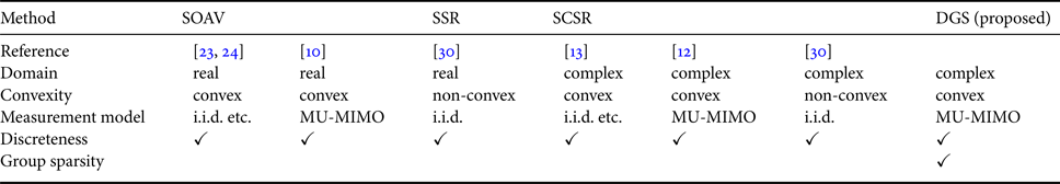
The use of the discreteness in the optimization problem has been proposed as the SOAV optimization [Reference Aïssa-El-Bey, Pastor, Sbaï and Fadlallah23, Reference Nagahara24], where the sum of $\ell _{1}$ norms is used as the regularizer for the discrete-valued vector. The idea of the SOAV optimization has been extended to the discrete-valued vector reconstruction in the complex-valued domain [Reference Hayakawa and Hayashi13]. Moreover, the extension to non-convex optimization has been proposed for both real- and complex-valued cases [Reference Hayakawa and Hayashi30]. The non-convex optimization in the real-valued domain is called sum of sparse regularizers (SSR) optimization. Such non-convex optimization-based approaches can achieve better performance than the convex ones in some cases. However, the convergence of the algorithm is not guaranteed for the non-convex optimization, and the performance is sensitive to the choice of the parameters.
The works in [Reference Hayakawa and Hayashi13, Reference Aïssa-El-Bey, Pastor, Sbaï and Fadlallah23, Reference Nagahara24, Reference Hayakawa and Hayashi30] do not focus on the signal detection in MU-MIMO systems, and hence the structure of the measurement matrix is different from the channel matrix considered in this paper. In [Reference Hayakawa and Hayashi30], for example, the ideal i.i.d. Gaussian matrix is used. To evaluate the performance in the MU-MIMO signal detection, the convex SOAV optimization and SCSR optimization have been applied to the scenario in [Reference Hayashi, Nakai, Hayakawa and Ha10, Reference Hayashi, Nakai-Kasai and Hayakawa12], respectively. The results show that the use of the discreteness by the convex optimization problems is effective also in the MU-MIMO signal detection.
The main advantage of the proposed DGS optimization against the above methods is to utilize the group sparsity of the unknown vector, which is preferable for the signal detection in IoT environments considered in this paper. Moreover, unlike [Reference Hayakawa and Hayashi30], the convergence of the proposed algorithm based on ADMM is guaranteed because the DGS optimization is convex.
IV. SIMULATION RESULTS
We evaluate the performance of the proposed signal detection methods via computer simulations. We assume the QPSK modulation with $1+j,-1+j,-1-j,1-j$ and set $(c_{1},c_{2},c_{3},c_{4},c_{5})=(0,1+j,-1+j,-1-j,1-j)$
 . The number of subcarriers is $Q=64$
 and the length of channel impulse response is $L=10$
 . We use $g_{1}(\cdot )=h_{1}(\cdot )$
 and $g_{\ell }(\cdot )=h_{2}(\cdot )$
 ($\ell =2,\dotsc ,5$
 ) as the sparse regularizers. In the simulations, the received signal $\boldsymbol {r}$
 and the channel matrix $\boldsymbol {A}$
 are scaled such that the scaled channel matrix $\tilde {\boldsymbol {A}}$
 satisfies $\lVert \tilde {\boldsymbol {A}} \rVert _{2}=1$
 . We set the parameter $\varepsilon$
 in the optimization problems (12) and (38) as $\sqrt {QM\sigma _{\text {v}}^{2}}$
 , where $\sigma _{\text {v}}^{2}$
 denotes the noise variance after the scaling. The parameter of ADMM is set to $\rho =1$
 . The number of inner iterations in ADMM is $K_{\text {itr}}=200$
 .
.
We investigate the initial parameters $q_{\ell }$ ($\ell =1,\dotsc ,S$
 ) and $\alpha$
 of the proposed IW-DGS in Algorithm 2. From the symmetry of the QPSK constellation, we can set $q_{2}=\dotsb =q_{5}$
 . Hence, we firstly tune the parameter $q_{1}$
 by evaluating the performance of the DGS optimization with $q_{2}=\dotsb =q_{5}=(1-q_{1})/4$
 . Figure 3 shows the SER performance of the proposed IW-DGS with $\alpha =20$
 versus $q_{1}$
 .In the figure, $T$
 denotes the number of outer iterations in IW-DGS. We assume the MU-MIMO OFDM system without precoding ($\boldsymbol {P}=\boldsymbol {I}_{Q}$
 ), where $(N,M)=(100,25)$
 , $N_{\text {act}}=15$
 and $E_{\text {b}}/N_{0}=15$
 dB. The figure shows that the best parameter in this case is $q_{1} = 0$
 , which means that we do not have to promote the sparsity of the transmitted symbol vector by the first regularizer $\sum _{\ell =1}^{S} \sum _{i=1}^{QN} q_{i,\ell } g_{\ell } \left ({x_{i} - c_{\ell }}\right )$
 in (38). This could be because the sparsity is sufficiently promoted by the second regularizer $\sum _{n=1}^{N} \alpha _{n} \left \lVert {\boldsymbol {x}_{n}}\right \rVert _{2}$
 in (38) when $\alpha _{n}>0$
 . We thus use $q_{1}=0$
 and $q_{2}=\dotsb =q_{5}=0.25$
 hereafter. Next, we examine the parameter $\alpha$
 to control the balance between the two regularizers. Figure 4 shows the SER performance of IW-DGS with $q_{1}=0$
 and $q_{2}=\dotsb =q_{5}=0.25$
 versus $\alpha$
 for $(N,M)=(100,40)$
 , $N_{\text {act}}=25$
 and $E_{\text {b}}/N_{0}=15\,{\rm dB}$
 . We can see that the SER performance of IW-DGS is significantly improved as $T$
 increases. Note that $\alpha =0$
 means that we do not utilize the group sparsity of the transmitted signal vector at all, and hence the DGS optimization with $\alpha =0$
 corresponds to the conventional SCSR optimization [Reference Hayakawa and Hayashi13]. The figure shows that we can significantly improve the SER performance by promoting the group sparsity with positive $\alpha$
 . This also means that the proposed DGS optimization can achieve much better performance than the conventional SCSR optimization. From the figure, we fix $\alpha =20$
 in the following simulations.
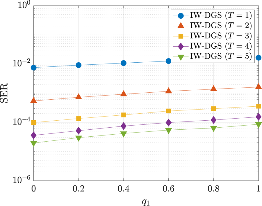
Fig. 3. SER performance of IW-DGS with $\alpha =20$ in MU-MIMO OFDM without precoding ($(N,M)=(100,25$
 ), $N_{\text {act}}=15$
 , $E_{\text {b}}/N_{0}=15\,{\rm dB}$
 ).
).
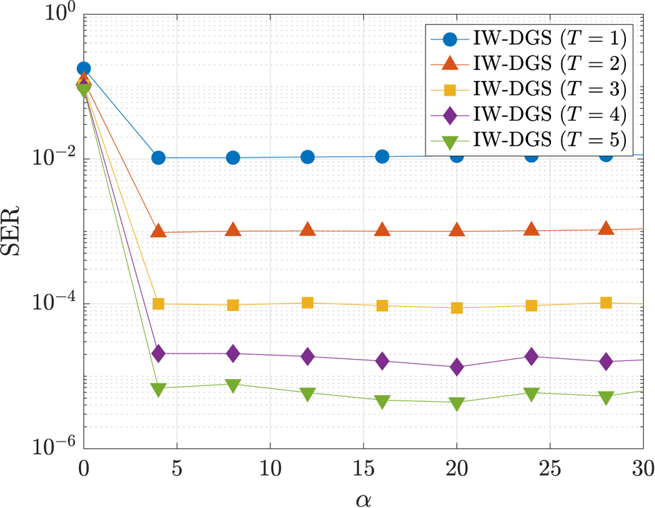
Fig. 4. SER performance of IW-DGS in MU-MIMO OFDM without precoding ($(N,M)=(100,40$ ), $N_{\text {act}}=25$
 , $E_{\text {b}}/N_{0}=15\,{\rm dB}$
 ).
).
Figures 5 and 6 show the SER performance of IW-DGS versus $E_{\text {b}}/N_{0}$ in MU-MIMO OFDM systems without precoding.We have $(N,M)=(50,25), N_{\text {act}}=10$
 in Fig. 5, and $(N,M)=(100,50), N_{\text {act}}=20$
 in Fig. 6. In the figures, ‘oracle ZF’ denotes the oracle ZF method, which perfectly knows the activity of each IoT terminal. Specifically, the estimate of the oracle ZF method is given by $\hat {\boldsymbol {s}}_{\text {act}}=(\boldsymbol {A}_{\text {act}}^{\mathsf {H}}\boldsymbol {A}_{\text {act}})^{-1}\boldsymbol {A}_{\text {act}}^{\mathsf {H}}\boldsymbol {r}$
 , where $\hat {\boldsymbol {s}}_{\text {act}} \in \mathbb {C}^{QN_{\text {act}}}$
 is the estimate of transmitted symbols of active IoT terminals and $\boldsymbol {A}_{\text {act}} \in \mathbb {C}^{QM \times QN_{\text {act}}}$
 is the corresponding submatrix of the whole channel matrix $\boldsymbol {A}$
 . We can see that the performance of IW-DGS with $T=10$
 is close to that of the oracle ZF, especially for larger-scale problems. Moreover, the proposed IW-DGS can achieve better performance than the oracle ZF for high $E_{\text {b}}/N_{0}$
 .
.
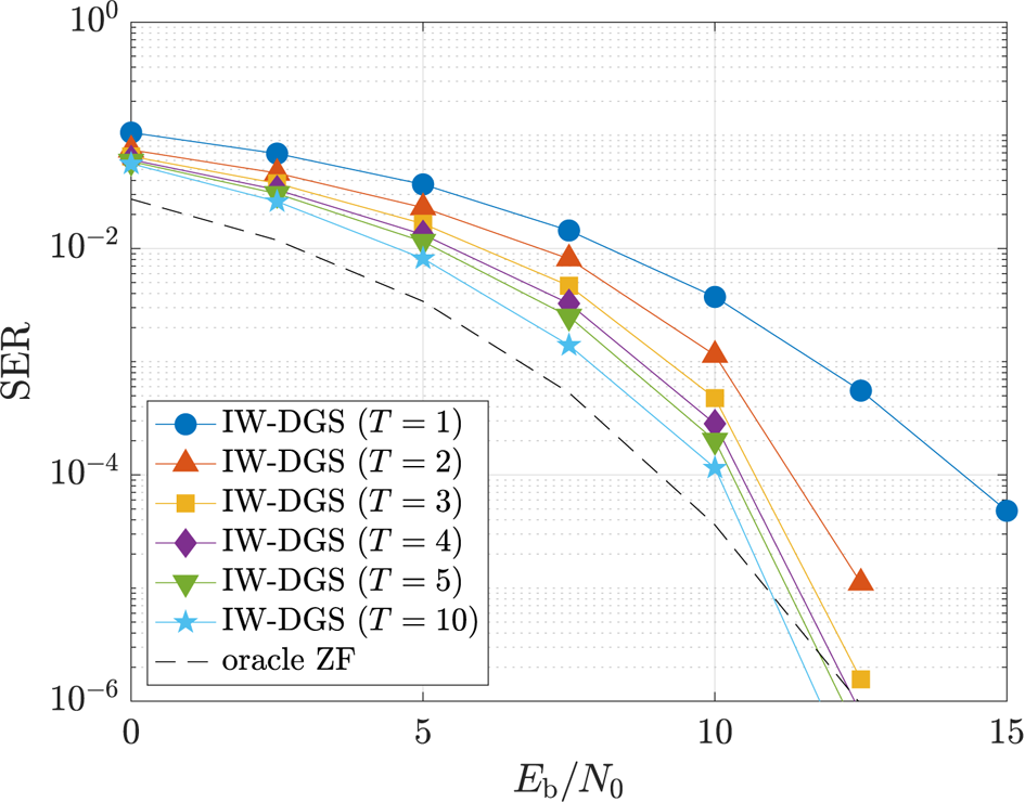
Fig. 5. SER performance of IW-DGS in MU-MIMO OFDM without precoding ($(N,M)=(50,25$ ), $N_{\text {act}}=10$
 ).
).

Fig. 6. SER performance of IW-DGS in MU-MIMO OFDM without precoding ($(N,M)=(100,50$ ), $N_{\text {act}}=20$
 ).
).
We then evaluate the effect of the precoding matrix $\boldsymbol {P}$ in MU-MIMO OFDM systems. Figure 7 shows the SER performance of IW-DGS versus $N$
 .We have $M=0.4N$
 , $N_{\text {act}}=0.3N$
 , and $E_{\text {b}}/N_{0}=15\,{\rm dB}$
 . In the figure, ‘non-precoded’ shows the SER performance when we do not use the precoding, i.e. $\boldsymbol {P}=\boldsymbol {I}_{Q}$
 . ‘Hadamard’ shows the performance with the precoding by the Hadamard matrix of order $Q$
 . ‘DFT’ shows the performance in the case with the DFT precoding, which is equivalent to MU-MIMO SC-CP systems. We can see that the performance in the precoded systems is much better than that in the non-precoded case. Even when $N=10$
 , we can achieve the SER of $10^{-4}$
 by using the precoding.
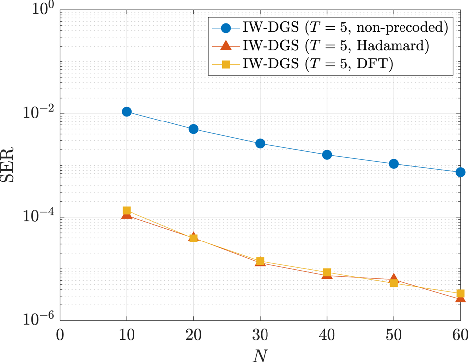
Fig. 7. SER performance of IW-DGS versus $N$ ($M=0.4N$
 , $N_{\text {act}}=0.3N$
 , $E_{\text {b}}/N_{0}=15\,{\rm dB}$
 ).
).
Finally, we show the SER performance versus $E_{\text {b}}/N_{0}$ in MU-MIMO SC-CP systems. Figure 8 shows the SER performance of IW-DGS in MU-MIMO SC-CP with $(N,M)=(50,25)$
 and $N_{\text {act}}=10$
 .We can see that the proposed IW-DGS with $T=10$
 can also achieve almost the same performance as the oracle ZF in this case.
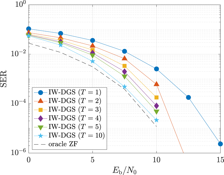
Fig. 8. SER performance of IW-DGS in MU-MIMO SC-CP ($(N,M)=(50,25$ ), $N_{\text {act}}=10$
 ).
).
V. CONCLUSION
In this paper, we have proposed the signal detection method for the uplink overloaded MU-MIMO systems for IoT environments. First, we have shown that the MU-MIMO SC-CP system can be regarded as the MU-MIMO OFDM system with the DFT precoding. Since the SC-CP approach requires neither IDFT operation nor precoding matrix multiplication at the transmitter side, it is suited to the IoT data collection scenario, where cost, capability, and energy of the transmitter are extremely limited. Moreover, PAPR of SC-CP signals is lower than that of OFDM signals. We then have proposed the signal detection method named IW-DGS, where we iteratively solve the W-DGS optimization with updating the parameters in the objective function. The proposed IW-DGS can utilize both the discreteness and the group sparsity of the transmitted signal vector. By using the structure of the channel matrix, we can reduce the order of the computational complexity of the proposed IW-DGS. Simulation results show that IW-DGS can achieve good performance close to the oracle ZF method in the overloaded scenarios, where the number of receiving antennas is less than that of IoT terminals. Moreover, by using the precoding with the Hadamard matrix or the DFT matrix, we can significantly improve the SER performance of the proposed method. Future work includes the extensive performance evaluation of the proposed method and extension to a non-convex optimization-based approach with the iterative weight update.
FINANCIAL SUPPORT
This work was supported in part by the Grants-in-Aid for Scientific Research no. 18K04148, and 18H03765 from the Ministry of Education, Culture, Sports, Science and Technology of Japan, the Grant-in-Aid for JSPS Research Fellow no. 17J07055 from Japan Society for the Promotion of Science, and the R&D contract (FY2017-2020) “Wired-and-Wireless Converged Radio Access Network for Massive IoT Traffic” (JPJ000254) for radio resource enhancement by the Ministry of Internal Affairs and Communications, Japan.This work was partially presented in APSIPA ASC 2018 [10] and 2019 [12].
STATEMENT OF INTEREST
None.
Ryo Hayakawa received the bachelor's degree in engineering, the master's degree in informatics, and the Ph.D. degree in informatics from Kyoto University, Kyoto, Japan, in 2015, 2017, and 2020, respectively. He is currently an Assistant Professor at the Graduate School of Engineering Science, Osaka University. He was a Research Fellow (DC1) of the Japan Society for the Promotion of Science (JSPS) from 2017 to 2020. He received the 33rd Telecom System Technology Student Award, APSIPA ASC 2019 Best Special Session Paper Nomination Award, and the 16th IEEE Kansai Section Student Paper Award. His research interests include signal processing and wireless communication. He is a member of IEEE and IEICE.
Ayano Nakai-Kasai received the B.E. and M.E. degrees from Kyoto University, Kyoto, Japan, in 2016 and 2018, respectively, where she is currently pursuing the Ph.D. degree with the Department of Systems Science, Graduate School of Informatics. Her research interests include signal processing and wireless communication. She received the Young Researchers’ Award from the Institute of Electronics, Information and Communication Engineers in 2018 and APSIPA ASC 2019 Best Special Session Paper Nomination Award. She is a member of IEEE and IEICE.
Kazunori Hayashi is currently a Professor at the Center for Innovative Research and Education in Data Science/Graduate School of Informatics, Kyoto University. He received the B.E., M.E., and Ph.D. degrees in communication engineering from Osaka University, Osaka, Japan, in 1997, 1999, and 2002, respectively. He was an Assistant Professor from 2002 to 2007, an Associate Professor from 2007 to 2017 at the Graduate School of Informatics, Kyoto University, and a Professor from 2017 to 2020 at the Graduate School of Engineering, Osaka City University. His research interests include statistical signal processing for communication systems. He received the ICF Research Award from the KDDI Foundation in 2008, the IEEE Globecom 2009 Best Paper Award, the IEICE Communications Society Best Paper Award in 2010, the WPMC’11 Best Paper Award, the Telecommunications Advancement Foundation Award in 2012, the IEICE Communications Society Best Tutorial Paper Award in 2013, and APSIPA ASC Best Special Session Paper Nomination Award in 2019. He is a member of IEEE, IEICE, and ISCIE.


 Open access