


1. Introduction
It is often informative to use simulation models that can predict changes in profitability of a range of production practices along with historical input and output prices to create a set of data that could then be analyzed to showcase how combinations of certain production factors impact estimated profitability over time. In these types of analyses, an attempt to draw conclusions about what individual factors, using combinations of input choices, have the largest impact on profitability is important to decision-makers facing similar situations as they would like to ascertain the input choices explaining the most variation in profits. A host of evaluation techniques exist for this purpose. Herein, we analyze artificial neural network (ANN) approaches and contrast results of their impact analyses to multivariate regression (MR) in terms of predictive accuracy and ability to identify relationships between production factors, historical prices, and associated profitability outcomes. At stake is transparency, consistency, and accuracy of results reported.
In this study, we use historical prices and weather data from the last two U.S. beef cattle cycles (1990–2003 and 2004–2014) and investigate estimated changes in profitability as a result of changing the herd size over time using a cow-calf simulation tool, the Forage and Cattle Analysis and Planning tool (FORCAP) as developed by Popp et al. (Reference Popp, Smith, Keeton and Maples2014). Prior studies suggest that managing the well-known concept of the cattle cycle to sell when prices are high and buy when price are low could lead to enhanced cow-calf producer returns (Bentley and Shumway, Reference Bentley and Shumway1981; Griffith, Burdine, and Anderson, Reference Griffith, Burdine and Anderson2017; Hamilton and Kastens, Reference Hamilton and Kastens2000; Lawrence, Reference Lawrence2002; Rosen, Reference Rosen1987; Tester et al., Reference Tester, Popp, Nalley and Kemper2019; Trapp, Reference Trapp1986). For this research, we rely on data from an analysis on herd size management (HSM) strategies most recently and intensively examined by Tester et al. (Reference Tester, Popp, Nalley and Kemper2019), where HSM practices varied from: (1) a strategy of holding the herd size constant regardless of price and weather conditions; (2) a countercyclical price signal-based strategy expanding/contracting the herd size when the short-term price outlook was weak/strong and hence would allow for capturing more sales when prices rebound/selling fewer head when prices would return to lower levels; and (3) a cost-based herd expansion strategy leading to herd size expansion when replacement heifers are relatively cheap and selling more replacement heifers when prices are high. Holding land resources constant, both fall- and spring-calving seasons and varying levels of fertility were analyzed in conjunction with HSM strategy (Table 1) and historical input and output prices (Table 2). Further, simulated weather impacts affected forage production, either creating conditions of excess hay sales or requiring purchase of hay to meet herd nutrition requirements (Table 3).
Table 1. Summary of input use and output changes across model runs for 1990–2014a

a Numbers are similar for subperiods but do vary because weather impacts and herd size changes were calculated differently. Prices varied more than forage production and herd size changes across subperiods. For details, please see Tester et al. (Reference Tester, Popp, Nalley and Kemper2019).
b Note that weather effects were modeled on a monthly basis such that good or bad weather at a particular time in a year could have deleterious or beneficial impacts (incl.) when compared to hay production without weather effects (excl.). For example, average hay sales were 46 for fall with most fertilizer use and no weather and increased to 58 with weather, whereas for spring, sales decreased from 119 to 109.
Table 2. Nominal Arkansas fertilizer, fuel, seed, and feed costs and cattle prices, 1990–2014
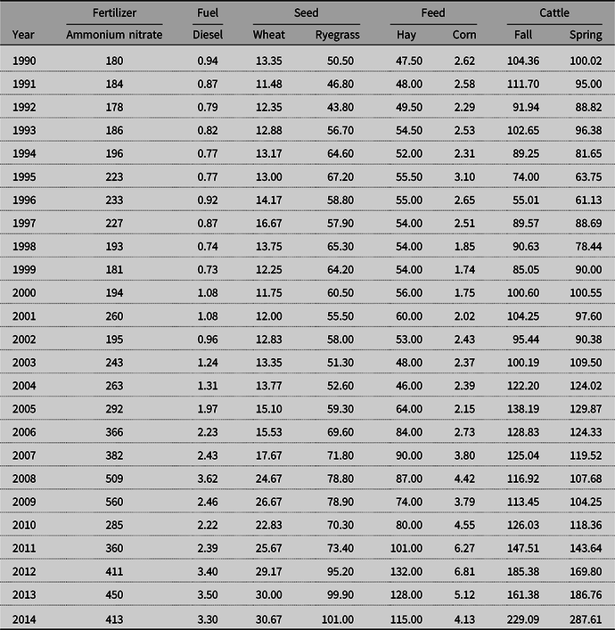
Note: Ammonium nitrate price is in $/ton, poultry litter price was constant at $23/ton, fuel is in $/gal., cattle price is in $/cwt. for 4-500 lb. steers in appropriate sale months of May and October for fall- and spring-calving herds, respectively, seed prices for planting of winter annuals are in $/cwt, hay prices are in $/ton, and supplemental feed corn prices are in $/lb.
Table 3. Sample of estimated gross receipts and direct costs of a 100-cow herd by calving season using 2005–2014 average prices with and without weather effects using the least fertilizer

Notes: Direct costs are organized more or less in order of occurrence during a production year, relative size, and whether or not they vary across systems. Seasonal price differences only impact cattle prices as input costs are only tracked on an annual basis. Weather conditions, on average, have been favorable for forage production over the course of the last 10 years in comparison to the 25-year average resulting in excess hay sales. Hay sales in combination with relatively high cattle prices for the past 10 years thereby have led to cash operating profit that is relatively high. Weaning, cull cow, and herd sire weights were held constant across calving season and were 555 lb. for steers, 520 lb. for heifers, 1,117 lb. for cows, and 1,850 lb. for herd sires. Cash operating profits are returns to land, labor, and capital. Differences in work hours with herd size changes, calving season, and weather are not accounted for.
With multiple variables impacting profitability of cow-calf operations over time, quantifying the relative impact of key variables on profitability is of aforementioned interest. The objective of this research was to estimate and rank the relative impacts of hay and cattle sales, level of fertilizer use, and calving season on cow-calf profitability using MR and ANNs. This was done for each cattle cycle and across the entire period (consistency). The point of comparing ANN to MR is to determine if using the more interpretable and the computationally easier MR approach (transparency) comes at the cost of sacrificing substantial explanatory power (accuracy). We quantify the magnitude of these trade-offs by calculating R 2 of in-sample profitability estimates and root-mean-square error (RMSE) for out-of-sample predictions using 10 randomly selected training and testing data sets that varied in size for each period. Further, knowledge of what factors drive profitability, regardless of computational method chosen, is important for producers so they can use this information to identify which factors to monitor most closely to maximize profit. Finally, producers may wish to know whether the impacts of factors change between the time periods analyzed: the cattle cycle from 1990 to 2003, the one from 2004 to 2014, or the entire period.
In order, we discuss (1) general insights about analytical techniques employed; (2) how the data were simulated and the models’ specifications; (3) the metrics to measure each independent variable’s explanatory power; (4) the implications of each independent variable’s impact in explaining profitability; and (5) conclusions.
2. Methods
2.1. Review of multivariate regression and artificial neural networks
Traditionally, regression analysis has been the foundational statistical technique for data analysis in applied economics. Regression analysis allows examination of the effects of one or more explanatory variables on a dependent variable where variables can be continuous, discrete, or categorical (Weisberg, Reference Weisberg2013). Regression results yield measures of statistical significance of hypothesized independent variables and then quantify those relationships using coefficient estimates that can ultimately be used to make predictions.
With the growth of big data and advanced artificial learning techniques, ANN analyses are becoming more popular as a viable alternative to traditional regression analysis. Despite demonstrated superior goodness of fit in many applications (Adya and Collopy, Reference Adya and Collopy1998; Ibrahim, Reference Ibrahim2013; Lek et al., Reference Lek, Delacoste, Baran, Dimopoulus, Lauga and Aulagnier1996; Warner and Misra,Reference Warner and Misra1996), ANN results are not easily interpreted when compared to regression analysis as ANN parameter estimates of explanatory variable effects on the dependent variable are often not revealed in a structured, user-defined manner but instead estimated as a neural network of relationships that are iteratively determined by weighting a myriad of functional forms (Olden and Jackson, Reference Olden and Jackson2002) and/or a variety of ANN configurations. Multi-layer feedforward (MLF) networks and generalized regression neural nets (GRNNs) are described here because they are relevant ANN configurations using Neural Tools v 7.5® (NT) software (Palisade Corporation, 2015b), an add-in to Excel®. MLF networks function through a backpropagation algorithm and include one or more hidden layers that specify the relationships between explanatory variables (Figure 1). These relationships are weighted to minimize the sum of squared prediction errors using a training process, involving iterations that require substantial processing time. The inclusion of more than one hidden layer increases complexity and often increases processing time so only one hidden layer was used. In general, the MLF method works well on large data sets with hundreds or thousands of observations. To make predictions, the user requires NT software because parameter estimates are hidden.
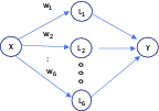
Figure 1. Multi-layer feedforward neural network diagram.
GRNN configurations are distinctly different from MLFs. Rather than manipulating relationships between explanatory variables and their connections to the dependent variable, GRNNs adjust a smoothness parameter to minimize the sum of squared prediction errors (Figure 2). The smoothness parameter determines the influence of observations on the predicted value as a function of their proximity to the desired output value obtained from the training set (University of Wisconsin, n.d.). Again, NT software is required for predictions but GRNNs often perform better for smaller data sets in comparison to MLFs.

Figure 2. Generalized regression neural network diagram with high (A) and low (B) smoothness parameter.
Further, NT and similar software exist to assist with the choice of (1) ANN framework to use (GRNN vs. MLFs with varying levels of nodes in a single hidden layer); and (2) the percentage of the original data set to use for training of the neural net versus the percentage used for testing predictions of the neural net. The user specifies the number of iterations used to minimize error in the training runs and the program picks random observations for training the neural net (Palisade Corporation, 2015b). As such, ANN outcomes can vary with the percentage of the data set used for training, the type of ANN (GRNN vs. MLF), and because the training data are chosen at random. Once a neural net is trained, however, “live” predictions are based on the estimated neural network for a given training percentage and given set of randomly drawn training data. However, a different training of the neutral network leads to different predictions, even with the same percent of observations and the same modeling technique (GRNN vs. MLF) used for training. Much like regression analysis, ANNs use the coefficient of determination (R 2) to measure explanatory power as well as RMSE for analyzing the predictive accuracy of the trained neural network on both the training and testing data set. We report RMSE for the testing data sets to assess predictive accuracy and R 2 on the training data sets to assess goodness of fit.
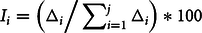
Further, NT reports relative impacts of explanatory variables on the dependent variable defined as follows (Palisade Corporation, 2015a):
 $${I_i} = \left({\Delta_i}\Big/\mathop \sum \nolimits_{i = 1}^j {\Delta_i}\right)\ * \ 100$$
where Δi is the difference between predicted maximum and minimum outcomes when changing the explanatory variable i across observations in the training data set holding all other explanatory variables constant and j is the number of explanatory variables. The i th impact on the dependent variable (I i) is then compared to the sum of all j explanatory variables’ impacts, calculated in the same way, to yield relative impacts for each explanatory variable that sum to 100% across all explanatory variables. This same approach is employed with outcomes from regression analysis as described in more in detail below.
2.2. Data
Combining modeled input use levels and output changes as summarized in Table 1 with changes in select input and output prices as shown in Table 2, cow-calf cash operating profits similar to those shown in Table 3 were estimated to provide annual profitability estimates as a function of combinations of 3 fertilizer use levels, 2 calving seasons, 25 production years, and 3 HSM strategies, each with and without weather effects on forage production for a total of 900 observations. Further, weather effects and HSM strategy vary slightly by subperiod chosen as average weather effects are impacted by length of period chosen. Also annual herd size change calculations for different HSM strategies vary by period. While details of impacts of these model outcomes are reported in Tester et al. (Reference Tester, Popp, Nalley and Kemper2019), Table 3 showcases typical results on profitability changes associated with calving season and the impact of weather. Fall calving is more profitable than spring calving given greater breeding failure rates associated with fescue toxicosis leading to fewer cattle sales with spring calving (Smith et al., Reference Smith, Caldwell, Popp, Coffey, Jennings, Savin and Rosenkrans2012). Hence, fall-calving herds exhibit higher sales given seasonally higher cattle sale prices as well as greater sales quantities (Table 2). Including weather effects altered hay sales, positively so, and more so in spring-calving operations given different monthly seasonal nutrition requirements. Herd nutrition requirements vary with calving season due to timing of feeding needs for replacement heifers and differences in gestational cow nutrition needs (Tester et al., Reference Tester, Popp, Nalley and Kemper2019—Tables 2 and 3). Adding herd size changesFootnote 1 for each year, using annual output and input prices, with different HSM strategies thus led to 1,650Footnote 2 annual, unique cow-calf operation simulations that were subsequently used to measure the relative impact of explanatory variables on operating profits as follows:
 $${Y_k} = {\alpha _0} + {\alpha _1}Hay{Q_k} + {\alpha _2}Hay{P_k} + {\alpha _3}Catt{Q_k} + {\alpha _4}Catt{P_k} + {\alpha _5}Fert{M_k} + {\alpha _6}Fert{H_k} \\ + {\alpha _7}Weathe{r_k} + {\alpha _8}Seaso{n_k} + \;{\varepsilon _k}$$
where Yk is cash operating profits in year k defined as the revenue generated from cattle and excess hay sales less production costs, HayQ k is the annual number of 1,200 lb. bales sold/bought, HayP k is the annual price of hay in dollars per ton, CattQ k is the yearly number of calves, cull cows, and cull bulls sold that varies both by HSM and by calving season, CattP k is the nominal 4-500 lb. steer priceFootnote 3 that varied by calving season (Table 2), FertM k and FertH k were binary (zero/one) variables denoting intermediate and highest fertilizer use (Table 1) in comparison to the least fertilizer use of the baseline, respectively, Weather k is a weather index indicating above/below cattle cycle or period-specific annual forage production that averages to 1 for a particular cattle cycle or period (for details, see Tester et al., Reference Tester, Popp, Nalley and Kemper2019), Season k is a binary variable for spring- or fall-calving season in a particular year, and ε k is the error term. Equation (2) was then estimated for each of the three time periods, the 1990–2003 cattle cycle, the 2004–2014 cattle cycle, and finally pooled over both time periods as weather effects were modeled using matching time periods, and hence forage production could vary given an upward trend in weather effects that led to greater forage production over time. Note that another specification could have included HSM strategy as a categorical explanatory variable instead of CattQ as the latter variable captures both calving season and HSM effects. However, the specification with the categorical HSM strategy variable instead of CattQ proved less powerful in terms of explaining profitability and thus this approach was not pursued.
2.3. Model specification
Since the variables, initially identified to impact profitability (Table 3), were strongly correlated leading to degrading multicollinearity (causing point estimates to be imprecise), principal component analysis was used to determine the appropriate number of explanatory variables in the regression model. Four principal components explained roughly 98% of the variation in the explanatory variables (Figure 3). This suggested the potential to eliminate several explanatory variables (1) using their statistical significance/contribution to model performance such that explanatory variables with |t-stat| < 1 were dropped (the adjusted R 2 criterion); and (2) by examining the extent of correlation among explanatory variables to avoid redundancy due to strong multicollinearity. The results suggested that hay price was statistically insignificant in every period analyzed, and that hay sold was highly correlated with weather as expected since the weather index drove forage production. Hay sold remained in the model given its ease of interpretation relative to the weather index and its larger |t-stat|. Finally, calving season was removed because the primary effect of a spring-calving season is higher expected breeding failures that result in fewer head sold. Therefore, head sold captured the majority of calving season effects, while cattle price captured seasonal price effects resulting from selling calves in the fall rather than the spring.
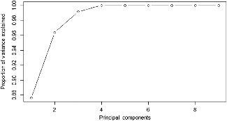
Figure 3. Principal component analysis for variable selection to explain cow-calf cash operating profits using hay and cattle sales, fertilizer use, calving season and weather over 1990–2014.
Additionally, ANN analysis was conducted using the initial set of explanatory variables. Similar to the regression results, the ANN model’s variable impact analysis revealed calving season, weather, and hay price to have little impact. Fertilizer was also shown to have little impact on the ANN, but provided substantial explanatory power in the regressions and therefore was included. Using these results, the final model specification included cattle price, hay sold, head sold, and fertilizer application level as follows:
 $${Y_k} = {\beta _0} + {\beta _1}Hay{Q_k} + {\beta _2}Catt{Q_k} + {\beta _3}Catt{P_k} + {\beta _4}Fert{M_k} + {\beta _5}Fert{H_k} + {\gamma _k}$$
where γ k is the error term and other variables are as described for equation (2). The set of explanatory variables was held constant across cycle (time period) as well as modeling technique.
2.4. Testing for consistency in neural network analysis results
Neural network analysis was conducted using NT (Palisade Corporation, 2015b). The “Best Net Search” tool was used to select the configuration that resulted in the lowest RMSE for training data sets that were separated by cycle or time period with the following results—GRNN for the 1990–2003 cycle, MLF with five nodes for the 2004–2014 cycle, and MLF with six nodes for the 1990–2014 period.
To test for the consistency of ANN modeling outcomes across cattle cycle and for the entire period, ANN analyses were repeated 10 times using training data sets that differed in size—two model runs with different randomly selected observations using 80%, 75%, 70%, 65%, and 60% of the data for training, holding modeling technique (GRNN, MLF with five nodes, or MLF with six nodes) constant for each of the time periods analyzed. This led to 10 observations of variable impacts and 10 estimates of R 2 per time period and per MR and ANN, to determine if the ranking of relative variable impacts changed across model runs and also by time period analyzed.
2.5. Compatibility of results between regression and neural network analyses
To allow comparison of R 2 and variable impact analyses between regression models and ANNs, randomly selected training data used in the ANN analyses were also used as the data set for regression analysis. For example, 403 random observations of the 504 observations in the 1990–2003 cycle (14 years × 2 calving seasons × 2 weather scenarios × 3 herd size strategies × 3 fertilizer use rates) were used in each of the two 80/20 training/testing data sets leading to 2 ANN and 2 MR variable impact outcomes using 2 different sets of randomly selected observations. Another two variable impact analyses for each of ANN and MR were then chosen using 75/25 training/testing data. Six further analyses for each of ANN and MR used 70/30 to 60/40 training/testing data sets by lowering the percentage of training data used by 5% and respectively raising the testing data set by 5%. Statistical significance of input variables was computed using heteroscedasticity-consistent standard errors using the coeftest function of the lmtest package for R (Zeileis and Horton, Reference Zeileis and Hothorn2002).
Finally, while R 2 was automatically reported for regression output, R 2 of ANN models were calculated using:
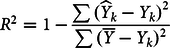 $${R^2} = 1 - {{\sum {{({\widehat Y_k} - {Y_k})}^2}} \over {\sum {{(\overline Y - {Y_k})}^2}}}$$
where  $\overline Y$ is the mean annual cash operating profitability (Y k) in the randomly selected training data sets for which a prediction $\widehat {{Y_k}}$ was made with number of observations changing by period and training/testing data set sizes.
Further, regression coefficients for each explanatory variable were used to estimate the variable’s impact on profitability for direct comparison to ANN analysis results. For example,
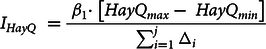 $${I_{HayQ}}{\rm{\;}} = {{{\beta _1} {\cdot} \;\left[ {Hay{Q_{max}} - \;Hay{Q_{min}}} \right]}\over{{\mathop \sum \nolimits_{i = 1}^j {\Delta_i}}}}$$
 was the relative impact of variable HayQ on Y (I HayQ), and Δ HayQ was calculated as shown in the numerator and represented the maximum change in  $\widehat {{Y}}$ with changes in HayQ, the difference between and largest and smallest observation, using coefficient estimates of equation (3), holding other variables constant, and i represented the ith of j explanatory variable impacts. Note that for the fertilizer effect, a binary zero/one variable, the maximum change $\widehat {{Y}}$ is reflected in the coefficient estimate of the highest fertilizer use dummy variable (FertH) and as such the fertilizer impact was calculated as follows:
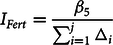 $${I_{Fert}} = {{{\beta _5}} \over {\sum\nolimits_{i = 1}^j {{\Delta _i}} }}$$
2.6. Nuances of estimating variable impacts
Variable impact can be estimated using varying metrics. Since FORCAP was used to generate the data analyzed herein, a large set of input values are used to estimate profit over time, that is, the costs of all relevant inputs, all relevant output prices and the implicit technology (production function) that, in this case, also includes the role of weather. Dixon, Garcia, and Anderson (Reference Dixon, Garcia and Anderson1987) demonstrated that conventionally estimated profit functions do not always result in good replications of underlying technology so that it is useful and informative to investigate alternative approaches. The underlying technologies in Dixon, Garcia, and Anderson (Reference Dixon, Garcia and Anderson1987) are smoothly continuous but those in FORCAP are not. This motivated the need to use alternative methods for ranking variable importance using ANNs and regression methods in a curve-fitting exercise. As noted earlier, conventional economic theory can be used to estimate derived demand from conventional profit functions. The models estimated below include outputs (cattle and hay) as well as their prices as independent variables. In the case of hay, its price serves as both an output price and an input price. Fertilizer price and other input prices are not included since they played a minor role on profitability as stocking rate changes and hay sales offset cost implications. By including hay and cattle output levels as well as fertilizer input use, both exogenous and endogenous variables in relation to profit are being included. Hence, it is not possible to impute any causal or behavioral relationships but simply measure via regression or ANN how profit varies as the explanatory variables (production, cattle prices, and input use) change. In essence, regression and ANNs are being used to estimate the shape of a more complex function and derive information about that more complex function.
3. Results
ANN models outperformed regression for any given sample by the R 2 criterion (Table 4). This was not surprising as neural networks examine a host of linear and nonlinear combinations of explanatory variables’ impacts on the outcome, whereas a linear functional form was used in the regression models (equation (3)). Across all time periods, R 2 values of ANN analyses ranged between 96.5 and 99.9%. In comparison, regression models generated a range of R 2 values from 89.3 to 92.8% using the same randomly selected training data sets as those used in ANN methods (Table 4). RMSE results were similar to R 2 results indicating that ANN methods have superior predictive accuracy in comparison to MR. All variables had a statistically significant impact at least at P = 0.001 in MR which was not surprising since a deterministic model was used to generate the dependent variable observations.
Table 4. Estimated effects of hay production, cattle sales, and fertilizer use on annual estimates of cow-calf cash operating profits using multivariate regression (MR) and comparison of R 2 and RMSE on testing data between MR and artificial neural network techniques of generalized regression neural networks (GRNNs) for 1990–2003, multi-layer feed forward (MLF) neural networks with 5 nodes for 2004–2014 and 6 nodes for 1990–2014 across 10 randomly selected training setsa by time period
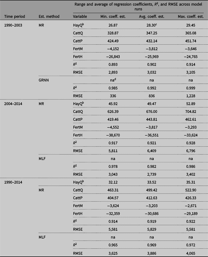
a Ten separate regression models for each time period, using different randomly selected subsamples of the data with different proportions used for training the neural net (60–80%). Randomly chosen observations were the same for MR versus GRNN or MLF analyses for each model run.
b HayQ was the annual number of 1,200 lb. bales sold or bought, CattQ was the yearly number of calves, cull cows, and cull bulls sold, CattP was the nominal, Arkansas average 4-500 lb. price for medium and large frame No. 1 steers.
c All model runs had coefficient estimates that were statistically significant at P < 0.001 including constant terms that are not reported.
d Not applicable. Relationship between variables and profitability not revealed.
For the first cattle cycle, 1990–2003, the ANN models identified cattle price as the most impactful variable (light shaded bars in Figure 4 top bar chart). Cattle price had an average impact of 52.1% compared to 19.0% for hay sold and was followed by head sold and fertilizer, respectively. Using MR, head sold was the most impactful variable and was followed by hay sold, fertilizer, and cattle price (darker shaded bars in Figure 4 top bar chart). Hay sold showed a slightly higher average impact over cattle price and fertilizer, but also had a larger range of impact estimates. Hence, aside from differences in goodness of fit (R 2) and RMSE, rankings of factors impacting profitability by magnitude of each factor’s variable impact, or importance ranking, varied by modeling technique for the first cattle cycle. Further, for all four variables, ANN models had a larger range of variable impacts compared to the MR models. This suggested that ANN modeling of dependencies between explanatory variables and the predicted outcome varied more by a particular training data set than changes in effects observed when a simple linear fit (MR) was imposed. Hence, ANN impact measures were less consistent than MR impact measures.
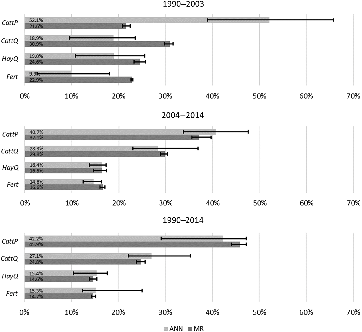
Figure 4. Comparison of variable impact analyses between artificial neural network (ANN) and multivariate regression (MR) methods: minimum, average, and maximum variable impacts as estimated across cycle or period are reflected in error bars using the same 10 different randomly selected training sets across method that varied in size from 60 to 80% in 5% increments.
For the second cycle, 2004–2014, cattle price remained the most impactful variable in every ANN model run with a noticeably smaller range in impacts compared to the first cattle cycle. In contrast with the previous cycle, head sold was more important than hay sold, while fertilizer remained the least impactful variable (middle bar chart of Figure 4). Importance rankings of variables using MR were similar to those of ANN analyses except for fertilizer use having greater impact than hay sales. Importance rankings based on MR, like ANN rankings, also varied with those reported for the first cattle cycle. Again, the range of ANN impacts was larger compared to those shown using MR. Since cattle made up the largest share of sales (Table 3) compared to hay sales, and since cattle prices were higher in the second cattle cycle compared to the first (Table 2), the changes in importance rankings make sense.
Lastly, over the entire period, 1990–2014, cattle price was again the most impactful variable using ANN analysis. Across periods analyzed, the margin between the impact of cattle price and the second most important factor was second largest (for the first period, the impact difference between the first and second factor was 33.2% on average, whereas it was 15.1% on average for the overall period). For the entire period, MR-based importance rankings, as during the second cycle, were close to ANN analyses results. Range of impacts was again larger for ANNs than MR results indicating ANNs led to less consistent results compared to MR.
4. Conclusions
Using a cow-calf simulation tool, FORCAP, this research sought to determine which of cattle price, head sold, hay price, hay bales sold, and fertilizer use would have the largest impact on profitability when analyzed over each of the last two cattle cycles or over the course of the last 25 years (two cycles combined). Nominal, annual profitability observations were simulated using annually varying input and output prices as well as changes in production practices that included: (1) level of fertilizer use that led to changes in forage production, with and without weather effects modeled that impact hay yields and also stocking rate; (2) modification of cow herd size over time; and (3) timing of calving season.
ANN analysis revealed cattle price to be the most impactful variable in every model run and analysis period, and MR similarly indicated cattle price was the most impactful variable in the second cycle and the overall period. Head sold was the second most impactful variable in ANN analysis with the exception of the first cycle where head sold ranked third. Quantity of hay sold was more important than fertilizer use across all periods. By comparison, MR results provided similar importance rankings except that (1) fertilizer use had a greater impact than hay sales for two of the three periods and (2) the importance ranking of cattle price and head sold was the opposite of that using ANN analysis in the first cattle cycle. A justification for head of cattle sold having a greater impact than cattle price in the first cycle could be that cattle prices were lower in the first cycle (Table 2), while variation in herd size across years in either of the two cattle cycles was similar although the timing of herd size changes varied by HSM strategy implemented.
Interestingly, ANN analysis results generated a larger range of variable impacts in every period when compared to MR. This highlights the criticism of ANNs that random selection of training observations and varying training set sizes lead to a large range of results even when using a consistent network configuration (GRNN vs. MLF with five or six nodes did not change across model runs). Hence, added goodness of fit with ANN compared to MR comes at the cost of more inconsistent impact results since the ANN results are more sensitive to the training sample chosen.
Should beef prices continue to rise as they did over the last 25 years, the analysis of the second cattle cycle results as well as the entire 25-year period imply cattle price, and head sold will be the most impactful variable determining profitability. Since cattle producers are price takers, production choices that impact cattle price received are limited to calving season management (purebred, organic, grassfed, and retained ownership are not analyzed here). Hence, preferring fall calving makes sense since calves born in fall can be sold as stocker cattle in the spring when forage production is plentiful and thereby a stocker price premium compared to calves sold in the fall when forages enter winter dormancy. The MR model found that increasing the number of head sold increased profits. This suggests that lower breeding failure rates and/or larger herd size would be profit-enhancing. However, more cattle consume more forage, hence greater cattle output implies lower hay sales and/or requires more fertilizer. One method to increase head sold without creating large increases in forage requirements (as calves get most of their nutrition from their mother’s milk) is to use fall calving with 14% fewer breeding failures than spring calving. Results from this analysis therefore reinforce both Smith et al.’s (Reference Smith, Caldwell, Popp, Coffey, Jennings, Savin and Rosenkrans2012) and Tester et al.’s (Reference Tester, Popp, Nalley and Kemper2019) conclusion that fall calving was the profit-maximizing choice for producers regardless of cattle cycle. However, the modeling conducted herein does not consider other factors outside the cow-calf haying enterprises on the farm. Many operations will have a poultry operation or even crop enterprises. There may well be labor limitations to moving to fall calving as crop harvest activities would interfere with calving season. Common in the mid-South is also a non-defined or year-round calving season (Doye, Popp, and West, Reference Doye, Popp and West2008) where controlled breeding allows lesser investment of time and facilities needed to keep herd sires from the herd.
Adding more fertilizer to increase forage production and thereby cattle or hay sales, on the other hand, showed pronounced negative effects in the MR model but they are offset by the resulting greater cattle and/or hay sales. However, these impacts are not easily discernable from the variable impacts reported by ANNs (Figure 4). Regression coefficients lend themselves more readily to examining this trade-off than ANN results. However, neither ANN- nor MR-based importance ranking results identify fertilizer at the medium level as profit-maximizing as demonstrated by Tester et al. (Reference Tester, Popp, Nalley and Kemper2019). Work by Smith et al. (Reference Smith, Popp, Keeton, West, Coffey, Nalley and Brye2016) suggests adding fertility to be of marginal value as well.
Tester et al. (Reference Tester, Popp, Nalley and Kemper2019) also found that the cost-based and cyclical price signal-based HSM strategies led to more head sold than a management practice of maintaining the herd at a constant size over time. Results from ANN and MR indicate that head sold is an important profitability factor. From a perspective of HSM strategy, the cost-based strategy, which led to the largest head of cattle sales compared to the cyclical price signal and constant herd size strategies, could thus erroneously be interpreted as the profit-maximizing decision when using ANN- or MR-based importance ranking results. Reduced excess hay sales with more cattle leads to sufficient revenue reduction or hay purchases that make such a strategy least profitable.
Similar to Adya and Collopy (Reference Adya and Collopy1998), Ibrahim (Reference Ibrahim2013), Lek et al. (Reference Lek, Delacoste, Baran, Dimopoulus, Lauga and Aulagnier1996), and Warner and Misra (Reference Warner and Misra1996), ANNs were a superior predictive technique as measured by R 2 and RMSE. This superior goodness of fit did come with a cost, however, as hidden layers are not revealed given the complexity of describing the relationships of a trained neural network. As such, model results for making predictions are useful only to those with access to software like NT. Retraining the network also led to changing results. Without an explicit description of relationships between explanatory variables and the dependent variable, as is available with MR in the form of magnitude and sign of parameter estimates, it is difficult to interpret results of a trained neural network in the absence of having access to the software’s prediction capabilities. With prediction capabilities, impacts of marginal changes in projected profitability, that likely change in sign and magnitude at different levels of the specific variable analyzed, can be estimated. Specifying a set of inputs and varying, for example, fertilizer application rate or number of head sold is a viable alternative to analyzing regression coefficients. This approach would allow for a variety of scenarios to be examined quickly, but also would require access to large amounts of data as well as software such as NT. This investment may be deemed appropriate by large producers whose management decisions have large financial implications, but for many producers, knowledge of regression coefficients may present sufficient information for making more informed decisions.
Finally, while we hint at the direction of future beef prices, results and conclusions of this research may not prove consistent for future time periods and geographic regions. For example, what would happen if all producers were to switch to fall calving? Likely, this would erode price premiums. Further, fall calving may not work in other regions, and seasonality in forage production may be different in other production regions. The FORCAP tool works well to predict conditions across the humid mid-Southern United States where both cool season and warm season forages can thrive. As such, results may be different for future cattle cycles and different production regions.
Nonetheless, results of this study suggest that ANNs are useful if accuracy of predicted outcomes is the end goal. Examination of profitability drivers, however, was more consistent with MR, and hence, for purposes of extension of research findings, MR is deemed to have an edge over ANN.
Financial support
This work was support by U.S. Department of Agriculture, National Institute of Food and Agriculture Hatch under project 02487.
Conflict of interest
None.


 Open access