


I. INTRODUCTION
Through a voice conversion (VC) [Reference Childers, Yegnanarayana and Wu1] system, voice characteristics of a source speaker can be transformed into those of the desired target speaker while still preserving the linguistic information. VC has been applied to various speech applications, such as for generation of speech databases with various voice characteristics [Reference Abe, Nakamura, Shikano and Kuwabara2, Reference Kain and Macon3], singing voice conversion (VC) [Reference Villavicencio and Bonada4, Reference Kobayashi, Toda and Nakamura5], the recovery of impaired speech signals [Reference Kain, Hosom, Niu, van Santen, Fried-Oken and Staehely6–Reference Doi, Toda, Saruwatari and Shikano8], expressive speech synthesis [Reference Inanoglu and Young9, Reference Türk and Schröder10], body-conducted speech processing [Reference Subramanya, Zhang, Liu and Acero11, Reference Toda, Nakagiri and Shikano12], and speech modification with articulatory control [Reference Tobing, Kobayashi and Toda13]. Furthermore, recent developments of anti-spoofing countermeasure systems [Reference Wu14, Reference Kinnunen15] have also employed VC systems for part of the spoofing data. Therefore, considering the benefits of VC, it is certainly worthwhile conducting a thorough study of the development of a high-quality VC system.
To perform VC, in general, two high-level features of a speech signal are used in the conversion, namely the voice-timbre and prosody characteristics. To convert the voice-timbre, one convenient way to do it is by transforming a compact representation of the vocal tract spectrum, such as mel-cepstrum features [Reference Tokuda, Kobayashi, Masuko and Imai16], through the use of a data-driven statistical mapping. Although there are several data-driven mapping for prosody transformation [Reference Wu, Kinnunen, Chng and Li17–Reference Sisman, Li and Tan19], in this work, we focus on the use of data-driven mappings for the conversion of spectral parameters. Finally, these transformed speech features are used to generate the converted speech, for example by using a vocoder-based waveform generation [Reference Dudley20–Reference Toda, Black and Tokuda22], or possibly by using a data-driven statistical waveform generation [Reference van den Oord23, Reference Tobing, Wu, Hayashi, Kobayashi and Toda24].
Indeed, in recent years, the development of data-driven VC systems have been rapidly proceeding, such as VC with a codebook-based method [Reference Abe, Nakamura, Shikano and Kuwabara2], with frequency-warping methods [Reference Erro, Moreno and Bonafonte25, Reference Godoy, Rosec and Chonavel26], with exemplar-based mappings [Reference Takashima, Takiguchi and Ariki27, Reference Wu, Virtanen, Chng and Li28], with statistical methods using Gaussian Mixture Model (GMM)-based approaches [Reference Kain and Macon3, Reference Toda, Black and Tokuda22, Reference Stylianou, Cappé and Moulines29], and with neural-network (NN)-based models [Reference Desai, Black, Yegnanarayana and Prahallad30–Reference Kaneko and Kameoka35]. In this work, considering the potential of NN-based methods, we focus on its use to perform the spectral conversion in VC, particularly with recurrent neural network (RNN) [Reference Hochreiter and Schmidhuber36, Reference Cho37], which can capture the long-term context dependencies. Note that different from recent works on the use of non-parallel (unpaired) data, such as with restricted Boltzmann machine [Reference Nakashika, Takiguchi and Minami33], variational autoencoder [Reference Hsu, Hwang, Wu, Tsao and Wang34], or generative adversarial network [Reference Kaneko and Kameoka35], in this work, we focus on the development of NN-based VC with parallel data. This is because in many cases it is still viable to collect a small amount of parallel data, i.e. where the source and target speakers utter the same set of sentences. Furthermore, established RNN-based modeling in parallel VC can be adapted for improving non-parallel methods.
As has been mentioned, in VC, to generate a converted speech waveform, a vocoder-based framework can be deployed, such as the mixed-excitation-based vocoders (STRAIGHT [Reference Kawahara, Masuda-Katsuse and De Cheveigné21], WORLD [Reference Morise, Yokomori and Ozawa38]). Other high-quality vocoders have also been developed, such as glottal-excitation-based vocoders [Reference Raitio39, Reference Airaksinen, Juvela, Bollepalli, Yamagishi and Alku40] and sinusoidal vocoders [Reference Erro, Sainz, Navas and Hernaez41, Reference Degottex, Lanchantin and Gales42]. A comparison of these vocoders on analysis–synthesis cases has also been made [Reference Airaksinen, Juvela, Bollepalli, Yamagishi and Alku40, Reference Morise and Watanabe43]. However, in cases where the speech features are estimated from a statistical model, such as from a text-to-speech (TTS) system, the performance of these vocoders is highly degraded [Reference Airaksinen, Juvela, Bollepalli, Yamagishi and Alku40, Reference Degottex, Lanchantin and Gales42]. The degradation in TTS, and possibly VC, applications are caused by the non-ideal conditions of the speech features estimated from a statistical model, such as oversmoothed condition of the spectral trajectory, where its variance is highly reduced due to the mean-based optimization [Reference Toda, Black and Tokuda22]. To overcome this problem, in this work, we investigate the use of the data-driven waveform generation method, which offers more potential in compensatory capability than the rule-based conventional vocoder.
Recently, a data-driven NN-based waveform generation method, using a deep autoregressive (AR) convolutional neural network (CNN) called WaveNet (WN) [Reference van den Oord23] has been proposed. WN models the waveform samples based on their previous samples using a stack of dilated CNNs to efficiently increase the number of receptive fields. In [Reference Tamamori, Hayashi, Kobayashi, Takeda and Toda44–Reference Adiga, Tsiaras and Stylianou46], auxiliary conditioning speech parameters, such as spectral and excitation features, are used to develop a state-of-the-art WN vocoder, which could generate meaningful speech waveforms with natural quality. However, as in a conventional vocoder, in VC [Reference Kobayashi, Hayashi, Tamamori and Toda47], WN still suffers from quality degradation due to the use of oversmoothed speech features, which introduces mismatches to the natural speech features used in training the model. To alleviate this problem, in this work, we presume that postprocessing methods [Reference Kobayashi, Toda and Nakamura5, Reference Toda, Black and Tokuda22, Reference Takamichi, Toda, Black, Neubig, Sakti and Nakamura48] will be more helpful in a WN vocoder, compared to the conventional vocoder, thanks to its data-driven characteristic for statistical compensation.
In this paper, to develop a better VC system, we employ the use of NN architectures for both spectral conversion modeling and waveform generation modeling. First, we perform an investigation on the use of RNN-based spectral conversion models compared to the conventional deep neural network (DNN) and deep mixture density network (DMDN) models [Reference Tobing, Wu, Hayashi, Kobayashi and Toda24] in a limited data condition. We show that our proposed RNN-based architecture could yield better performance, and it naturally can capture long-term context dependencies in training and mapping stages. Furthermore, to improve the condition of the generated spectral trajectory, we also propose to use spectrum differential loss for the RNN-based model training, which is based on a synthesis/postfilter approach using direct waveform modification with spectrum differential (DiffVC) [Reference Kobayashi, Toda and Nakamura5]
Lastly, to improve the statistical waveform modeling with a WN vocoder in VC, we propose several postprocessing methods that alleviate the possible mismatches and oversmoothness of the estimated speech features. These postprocessing methods are based on global variance (GV) postfilter [Reference Toda, Black and Tokuda22] and the DiffVC method [Reference Kobayashi, Toda and Nakamura5]. In the future, it would be better to avoid the use of such postprocessing techniques and directly address the feature mismatches by utilizing the data-driven traits of a statistical waveform model. Indeed, in both TTS [Reference Shen49] and VC [Reference Liu, Ling, Jiang, Zhou and Dai50], such a concept has been applied, where text/linguistic features are used, which may not be available in every practical situation. In this work, as the first step toward the improvement of a more flexible text-independent VC system, we perform investigations on the capability of statistical waveform modeling with postprocessing techniques.
To recap, in this paper, our contributions are twofold: to develop an RNN-based spectral conversion model that is better than the conventional DNN architectures, and to investigate the effects of several postprocessing methods for improving the use of WN vocoder in VC. In the experimental evaluation, it has been demonstrated that: (1) the proposed RNN-based spectral modeling architecture achieved better performance than the conventional DNN/DMDN architectures even with limited training data; (2) the proposed spectrum differential loss in RNN-based modeling further improves the naturalness of converted speech in same-gender conversions; and (3) the proposed post-conversion processing yields the best naturalness and conversion accuracy of converted speech compared to the conventional use of WN vocoder. Henceforth, the main motivation of this work is to better understand the effectiveness of using NN-based feature modelings, such as for spectral mapping, and waveform generation, i.e. neural vocoder, through careful evaluations and investigations toward further improvements of these core techniques.
The remainder of this paper is organized as follows. In Section II, a brief overview of the proposed systems and their correlation with the previous work are described. In Section III, the proposed NN-based architectures for the spectral mapping models are elaborated. In Section IV, the WN vocoder used as the NN-based waveform model is explained, as well as the proposed method for alleviating the quality degradation in VC. In Section V, objective and subjective experimental evaluations are presented. Finally, the conclusion of this paper is given in Section VI.
II. COMPARISON TO PREVIOUS WORK
In this work, we describe our method for a VC system with the use of NN-based statistical models for both spectral mapping and waveform generation. This idea was incorporated in our previous VC system [Reference Tobing, Wu, Hayashi, Kobayashi and Toda24], which participated in the VCC 2018 [Reference Lorenzo-Trueba51]. The previous system [Reference Tobing, Wu, Hayashi, Kobayashi and Toda24], which was ranked second in the challenge, used a DMDN-based model [Reference Zen and Senior52] for the spectral mapping and a WN vocoder to generate the converted speech. To alleviate the degradation problem in WN, a post-conversion processing based on the DiffVC and GV (DiffGV) was used to obtain refined auxiliary speech features for the WN vocoder. However, there still exist several limitations on our previous work, which include (1) the need of using a separate module in the DMDN-based model to incorporate time-dependency in spectral trajectory generation, i.e. maximum likelihood parameter generation (MLPG) [Reference Toda, Black and Tokuda22, Reference Tokuda, Kobayashi and Imai53]; (2) no empirical observations that prove the DiffGV post-conversion processing is better than either solely DiffVC- or GV-based; and (3) a possibility of better spectral modeling with spectrum differential loss to preserve the consistency with DiffGV method, which uses spectrum differential features in its process.
To build on our previous work, first, we propose to improve the spectral mapping modeling, as illustrated in the upper diagram of Fig. 1, as follows: (1) by using RNN-based architecture, which can naturally capture long-term context dependencies, and (2) by using spectrum differential loss in parameter optimization to preserve the consistency with the DiffGV method, which may improve the condition of generated spectral trajectory. To clearly describe these methods, we first elaborate on the DNN- and DMDN-based spectral mapping models [Reference Tobing, Wu, Hayashi, Kobayashi and Toda24, Reference Zen and Senior52]. We also describe the RNN-based architectures for spectral mapping with long-short term memory (LSTM) [Reference Hochreiter and Schmidhuber36] or with a gated recurrent unit (GRU) [Reference Cho37]. Finally, these spectral mapping models are objectively evaluated in a limited training data condition, where it has been demonstrated that the GRU-based spectral modeling yields better performance than the others. Note that we focus on comparing the LSTM- and GRU-based spectral modeling in a basic VC task to confirm the effectiveness of a more compact GRU architecture, which is more beneficial for real-world applications.
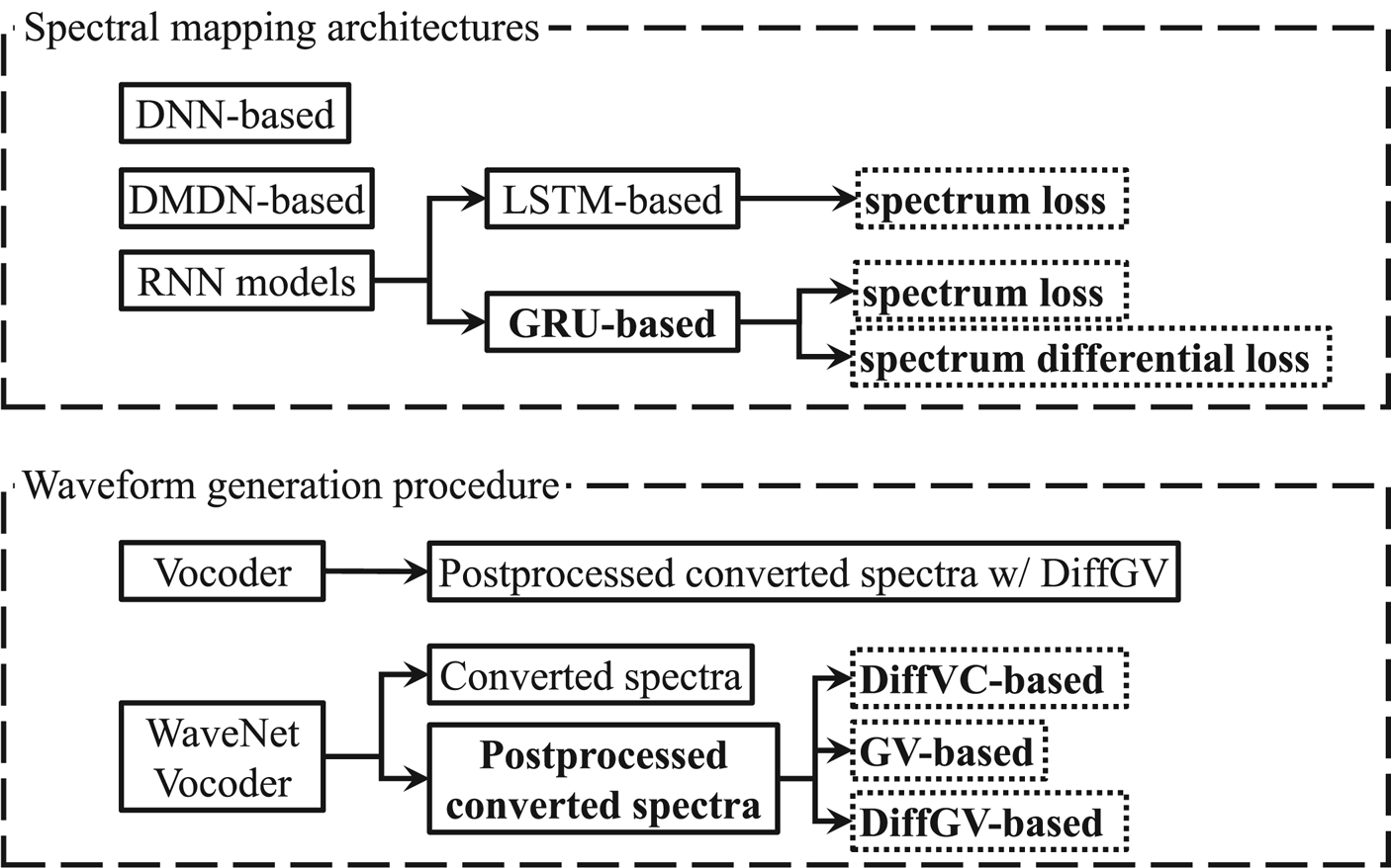
Fig. 1. Diagram of the overall flow and contribution of the proposed work. Bold denotes proposed methods and dashed boxes denote proposed experimental comparisons. Arrow denotes a particular implementation detail of its parent module.
Secondly, we propose to investigate the effect of several post-conversion processing methods, i.e. with DiffVC-, with GV-, or with DiffGV-based post-conversions, for the WN vocoder in VC. We also compare these methods with the conventional vocoder framework that uses DiffGV-based post-processed speech features, as illustrated by the lower diagram of Fig. 1. In the experimental evaluation, it has been demonstrated that the DiffGV-based post-conversion with WN vocoder yields superior performance compared to the others. Further, coupled with the use of the proposed spectrum differential loss in the spectral mapping model, the proposed method yields higher performance in the same-gender conversions.
III. SPECTRAL CONVERSION MODELS WITH NN-BASED ARCHITECTURES
This section describes the NN-based spectral mapping models used for the VC framework in this paper. These include the DNN and DMDN [Reference Zen and Senior52], which are optimized according to the conditional probability density function (PDF) of the target spectral features, given the input source spectral features. Compare to the straightforward DNN architecture, the DMDN has the advantage of being capable of modeling a more complex distribution of the target features, as well as to model not only their means but also their variances. In the DNN and DMDN, a separate MLPG module [Reference Toda, Black and Tokuda22, Reference Tokuda, Kobayashi and Imai53] is used after the conversion network to generate the estimated spectral trajectory. Finally, we also elaborate on the RNN-based spectral mapping models, where, in contrast to the DNN/DMDN models, all components can be optimized during training.
Let $\boldsymbol {x}_t=[x_t(1),\dotsc ,x_t(d),\dotsc ,x_t(D)]^{\top }$ and $\boldsymbol {y}_t= [y_t(1),\dotsc ,y_t(d),\dotsc ,y_t(D)]^{\top }$
 be the $D$
 -dimensional spectral feature vectors of the source speaker and target speaker, respectively, at frame $t$
 . Their 2D spectral feature vectors are, respectively, denoted as $\boldsymbol {X}_t=[\boldsymbol {x}_t^{\top },\Delta \boldsymbol {x}_t^{\top }]^{\top }$
 and $\boldsymbol {Y}_t=[\boldsymbol {y}_t^{\top },\Delta \boldsymbol {y}_t^{\top }]^{\top }$
 , where $\Delta \boldsymbol {x}_t$
 and $\Delta \boldsymbol {y}_t$
 are the corresponding delta features, which capture the rate of change of values between successive feature frames.
A) Spectral conversion with DNN
In the DNN, given an input spectral feature vector $\boldsymbol {X}_t$ at frame $t$
 , the conditional PDF of the target spectral feature vector $\boldsymbol {Y}_t$
 is defined as

where $\mathcal {N}(\cdot; \boldsymbol {\mu },\mathbf {\Sigma })$ denotes a Gaussian distribution with a mean vector $\boldsymbol {\mu }$
 and a covariance matrix $\mathbf {\Sigma }$
 . $\boldsymbol {D}$
 is the diagonal covariance matrix of the target spectral features computed using the training dataset beforehand. The set of parameters of the network model is denoted as $\boldsymbol {\lambda }_S$
 , and $f_{\boldsymbol {\lambda }_S}(\cdot )$
 is the feedforward function of the network.
In the training phase of the DNN network, to estimate the updated model parameters $\hat {\boldsymbol {\lambda }}_S$ , backpropagation is performed throughout the network to minimize the loss function as follows:

where $\top$ denotes the transpose operator and $T$
 denotes the total number of time frames.
Then, using the trained DNN network model, a spectral conversion function can be applied to generate the estimated target spectral trajectory $\hat {\boldsymbol {y}}=[\hat {\boldsymbol {y}}_1^{\top },\hat {\boldsymbol {y}}_2^{\top },\dotsc ,\hat {\boldsymbol {y}}_t^{\top },\dotsc , \hat {\boldsymbol {y}}_T^{\top }]^{\top }$ by using the MLPG [Reference Toda, Black and Tokuda22, Reference Tokuda, Kobayashi and Imai53] procedure as follows:

where $\boldsymbol {M}=[f_{\boldsymbol {\lambda }_S}(\boldsymbol {X}_1)^{\top },f_{\boldsymbol {\lambda }_S}(\boldsymbol {X}_2)^{\top }, \dotsc ,f_{\boldsymbol {\lambda }_S}(\boldsymbol {X}_t)^{\top },\dotsc , f_{\boldsymbol {\lambda }_S}(\boldsymbol {X}_T)^{\top }]^{\top }$ is the sequence of network outputs, and $\overline {\boldsymbol {D}}^{-1}$
 denotes a sequence of inverted matrices of the diagonal covariance $\boldsymbol {D}$
 . The transformation matrix is denoted as $\boldsymbol {W}$
 , which is used to enhance a sequence of spectral feature vectors with its delta feature contexts, i.e. the rate of change of values between successive feature frames.
B) Spectral conversion with DMDN
For DMDN-based [Reference Zen and Senior52] spectral conversion, given an input spectral feature vector $\boldsymbol {X_t}$ at frame $t$
 , the conditional PDF of the target spectral feature vector $\boldsymbol {Y}_t$
 is defined as a mixture of distributions as

where the Gaussian distribution is denoted as $\mathcal {N}(\cdot; \boldsymbol {\mu },\mathbf {\Sigma })$ with a mean vector $\boldsymbol {\mu }$
 and a covariance matrix $\mathbf {\Sigma }$
 . The index of the mixture component is denoted by $m$
 and the total number of mixture components is $M$
 . The set of model parameters is denoted as $\boldsymbol {\lambda }$
 . The time-varying weight, mean vector, and diagonal covariance matrix of the $m$
 th mixture component are, respectively, denoted as $\alpha _{m,t,\boldsymbol {\lambda }}$
 , $\boldsymbol {\mu }_{m,t,\boldsymbol {\lambda }}$
 , and $\mathbf {\Sigma }_{m,t,\boldsymbol {\lambda }}$
 . These time-varying mixture parameters are taken from the network output

To estimate the updated model parameters $\hat {\boldsymbol {\lambda }}$ in the training of a DMDN-based spectral conversion model, backpropagation is performed according to the following negative log-likelihood function:

Similar to the DNN, in the conversion phase, the estimated target spectral trajectory $\hat {\boldsymbol {y}}$ is generated by using the MLPG [Reference Toda, Black and Tokuda22, Reference Tokuda, Kobayashi and Imai53] procedure as follows:

where the transformation matrix used to append the spectral feature vector sequence with its delta features is denoted as $\boldsymbol {W}$ . The sequence of mixture-dependent time-varying inverted diagonal covariance matrices is denoted as $\overline {\mathbf {\Sigma }_{\hat {\boldsymbol {m}}}^{-1}}$
 and that of the mean vectors is denoted as $\overline {\boldsymbol {\mu }_{\hat {\boldsymbol {m}}}}$
 . The suboptimum mixture component sequence, which is denoted as $\hat {\boldsymbol {m}}=\{\hat {m}_1,\hat {m}_2,\dotsc ,\hat {m}_t,\dotsc ,\hat {m}_T\}$
 , used to develop the respective sequences of time-varying mixture parameters is determined as

Note that both (3) and (6) generate the estimated $D$ -dimensional target feature vector sequence $\hat {\boldsymbol {y}}$
 , whereas the input to the network is 2D input feature vector $\boldsymbol {X}_t$
 at each time $t$
 . This is because the network actually outputs 2D feature vector for DNN, i.e. $f_{\boldsymbol {\lambda }_S}(\boldsymbol {X}_t)$
 , or $M$
 sets of 2D mean vector $\boldsymbol {\mu }_{m,t,\boldsymbol {\lambda }}$
 and diagonal covariance matrix $\rm {diag}(\mathbf {\Sigma }_{m,t,\boldsymbol {\lambda }})$
 for DMDN at each time $t$
 , where they were then processed by the MLPG procedure to generate the spectral trajectory by considering their temporal correlation. This kind of explicit treatment can be alleviated by directly incorporating the use of network architecture with temporal modeling capabilities, such as RNN, which is described in the following section.
C) Spectral conversion with RNN
It is also important to note that a speech signal, and thus its parametrization, is time-sequence data. Therefore, it would be more reasonable to develop a spectral conversion model that is capable of capturing the dependencies within a sequence of spectral feature vectors, such as by using the RNN architectures. Hence, we propose the use of LSTM [Reference Hochreiter and Schmidhuber36] and a GRU [Reference Cho37] as the basis RNN units used to capture the long-term context dependencies on the input spectral features. The flow of the RNN-based spectral modeling is shown in Fig. 2. It can be observed that additional convolutional input layers are also used to extract better contextual input frames. Note that, different from the previous DNN/DMDN architectures, in the proposed RNN-based spectral conversion models, all of the components, except for the normalization and denormalization layers (which are kept fixed to make the network work with the normalized values of the features), are optimized during training.
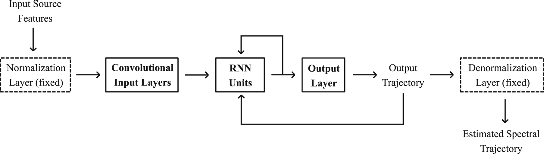
Fig. 2. Spectral mapping model with RNN-based architectures.
1) LSTM-based spectral conversion model
Given an input spectral feature vector $\boldsymbol {x}_t$ at frame $t$
 , the estimated target spectral feature vector $\hat {\boldsymbol {y}}_t$
 is estimated as

where $\boldsymbol {W}_{hy}$ and $\boldsymbol {b}_{y}$
 , respectively, denote the weights and biases of the output layer in Fig 2. The hidden state $\boldsymbol {h}_t$
 is produced by the LSTM units [Reference Hochreiter and Schmidhuber36] as follows:


where $\hat {\boldsymbol {y}}_0 = \boldsymbol {0}$ . The cell state is denoted as $\boldsymbol {c}_t$
 . The input, forget, cell, and output gates are denoted as $\boldsymbol {i}_t$
 , $\boldsymbol {f}_t$
 , $\boldsymbol {g}_t$
 , and $\boldsymbol {o}_t$
 , respectively. The trainable weights and biases are denoted by the corresponding $\boldsymbol {W}$
 and $\boldsymbol {b}$
 , respectively. $\sigma$
 denotes a sigmoid function and $\odot$
 denotes an element-wise product.
The network model parameters $\hat {\boldsymbol {\lambda }}_\textrm {R}$ are optimized through backpropagation for the loss function, computed by considering the distortions in the mel-cepstrum domain [Reference Mashimo, Toda, Shikano and Campbell54], as follows:

where $|\cdot |$ denotes the absolute function. The $d$
 th dimension estimated spectral feature at time $t$
 is denoted as $\hat {y}_t(d)$
 , where the estimated spectral feature vector $\hat {\boldsymbol {y}}_t$
 can be written in terms of the feedforward function in an RNN-based spectral mapping model as $f_{\boldsymbol {\lambda }_\textrm {R}}(\boldsymbol {x}_t)=[\hat {y}_t(1),\hat {y}_t(2),\dotsc ,\hat {y}_t(d),\dotsc ,\hat {y}_t(D)]^{\top }$
 . Note that the input source spectra $\boldsymbol {x}_t$
 is firstly fed into the input convolutional layers before being fed into the RNN units as shown in Fig. 2.
2) GRU-based spectral conversion model
In addition to modeling the long-term context dependencies, it is also worthwhile considering a more compact model architecture, such as the GRU [Reference Cho37] units, which will be more suitable for our purpose in using a small amount of training data. A more compact network will also be more suitable for real-time applications, which require low-latency computation.
In the proposed GRU-based spectral conversion model, given an input spectral feature vector $\boldsymbol {x}_t$ at frame $t$
 , the following functions are computed by the GRU units:


where $\hat {\boldsymbol {y}}_t$ is given by (8) and, similarly, $\hat {\boldsymbol {y}}_0=\boldsymbol {0}$
 . The hidden state of the GRU is denoted as $\boldsymbol {h}_t$
 . The reset, update, and new gates are denoted as $\boldsymbol {r}_t$
 , $\boldsymbol {z}_t$
 , and $\boldsymbol {n}_t$
 , respectively. The corresponding weights and biases are, respectively, denoted by $\boldsymbol {W}$
 and $\boldsymbol {b}$
 . The sigmoid function is denoted by $\sigma$
 and $\odot$
 denotes an element-wise product. As in the LSTM-based model, for multiple layers of GRU units, the hidden state of the current layer is used as the input for the succeeding layer. As can be observed, the modeling of long-term context dependencies in GRU is achieved through fewer computation steps, and model parameters, compared to the LSTM, which might be better for limited data situations and real-time computation.
IV. WAVEFORM GENERATION MODELS WITH WN VOCODER
In this paper, in addition to the spectral conversion models, we also employ an NN-based architecture for the waveform generator (neural vocoder), i.e. the WN [Reference van den Oord23] model. As a first step towards the generalization of the use of other neural vocoders in VC, we describe the use of WN vocoder [Reference Tamamori, Hayashi, Kobayashi, Takeda and Toda44–Reference Adiga, Tsiaras and Stylianou46], where the WN model is conditioned using both speech waveform samples and extracted speech parameters. We address the quality degradation problem faced by the WN vocoder in VC when it utilizes estimated speech parameters [Reference Kobayashi, Hayashi, Tamamori and Toda47] from a spectral conversion model, through a post-conversion processing [Reference Tobing, Wu, Hayashi, Kobayashi and Toda24]. Finally, we propose a modified loss function in the development of the spectral conversion model to preserve the consistency with the waveform generation procedure.
A) WN vocoder
WN [Reference van den Oord23] is a deep AR-CNN that is capable of modeling speech waveform samples for their previous samples. To efficiently increase the number of receptive fields of waveform samples, WN uses a stack of dilated CNNs using residual blocks, making it possible to produce human-like speech sounds. Moreover, when it is conditioned with naturally extracted speech features, such as spectral and excitation parameters, a WN vocoder [Reference Tamamori, Hayashi, Kobayashi, Takeda and Toda44–Reference Adiga, Tsiaras and Stylianou46] is capable of producing meaningful speech waveforms with the natural quality compared with the conventional vocoder framework.
Given a sequence of auxiliary feature vectors $\boldsymbol {h}=[\boldsymbol {h}_1^{\top },\boldsymbol {h}_2^{\top },\dotsc ,\boldsymbol {h}_t^{\top },\dotsc ,\boldsymbol {h}_T^{\top }]^{\top }$ , the likelihood function of a sequence of the corresponding waveform samples $\boldsymbol {s}=[s_1,s_2,\dotsc ,s_t,\dotsc ,s_T]^{\top }$
 is given by

where the conditional PDF of a waveform sample $P(s_t|\boldsymbol {h}_t,\boldsymbol {s}_{t-p})$ is modeled by the WN vocoder, and $\boldsymbol {s}_{t-p}$
 denotes the previous samples with $p$
 receptive fields. In the training, the ground-truth previous samples are given, i.e. teacher-forcing mode, whereas, in the synthesis phase, the waveform is generated sample-by-sample. Note that the modeling of the waveform samples in a WN vocoder can be performed as a classification problem, where the floating values of the 16-bit waveform will be discretized into 256 categories using the $\mu$
 -law algorithm. The inverse $\mu$
 -law algorithm is used in synthesis after sampling from the output distribution.
B) Postconversion processing in VC
In VC, to use the WN vocoder, estimated speech features, generated from a statistical mapping model, such as the ones described in Section III, are fed as auxiliary conditioning features in equation (20) to generate the converted speech waveform. However, in this case, the WN vocoder will face a significant degradation [Reference Kobayashi, Hayashi, Tamamori and Toda47], because of the mismatches of speech features, such as the oversmoothed characteristics of the estimated spectral features due to the mean-based optimization of a spectral conversion model. To improve the quality of the converted speech waveform, these mismatches between the naturally extracted speech parameters and the oversmoothed estimated speech parameters have to be alleviated, e.g. with a post-conversion processing method.
The ideal way to address the degradation problem of WN vocoder in VC is by directly addressing the mismatches of speech features in the development of a WN vocoder. In this work, as a first step toward improving the use of the neural vocoder in VC, we propose to overcome the quality degradation by the use of post-conversion processing to alleviate the feature mismatches, such as oversmoothing problem. The proposed post-conversion processing is based on GV [Reference Toda, Black and Tokuda22] postfilter and DiffVC [Reference Kobayashi, Toda and Nakamura5], which is illustrated in Fig. 3. The GV postfilter is used to recover the variances of the oversmoothed spectral features to make them closer to the natural ones. The DiffVC method is used to further reduce the mismatches between the spectral and excitation features by directly modifying the input speech waveform according to the differences between the estimated target spectra and the input spectra. Then, through the combination of GV and DiffVC post-conversion processing (DiffGV), the modified set of speech parameters [Reference Tobing, Wu, Hayashi, Kobayashi and Toda24] can be obtained for use in the WN vocoder as shown in Fig. 4. Note that, as shown in Fig. 3, for cross-gender conversions, e.g. male-to-female speakers, an additional step of analysis–synthesis is performed with also the transformed excitation features because the DiffVC [Reference Kobayashi, Toda and Nakamura5] method does not modify the original excitation when filtering to generate the modified waveform using the mel-log spectrum approximation (MLSA) filter [Reference Imai, Sumita and Furuichi55].
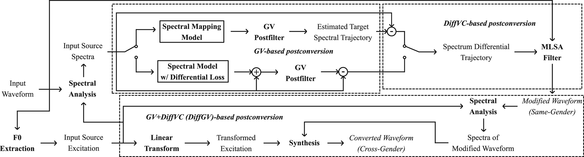
Fig. 3. Flow of direct waveform modification with spectrum differential (DiffVC) [Reference Kobayashi, Toda and Nakamura5] using MLSA synthesis filter [Reference Imai, Sumita and Furuichi55] and GV postfilter [Reference Toda, Black and Tokuda22].
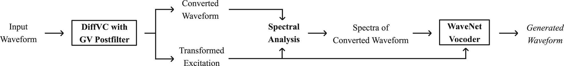
Fig. 4. Waveform generation procedure for converted speech using WN vocoder through the use of post-conversion processed auxiliary speech features based on the DiffVC method and the GV postfilter (DiffGV).
Finally, to preserve the consistency between the spectral conversion model and the waveform generation procedure, due to the use of spectrum differential method (DiffVC), we propose the use of an alternative loss function for the RNN-based architectures that considers the spectrum differences. Given the estimated feature vector $\hat {\boldsymbol {y}}_t=f_{\boldsymbol {\lambda }_\textrm {R}}(\boldsymbol {x}_t)$ from (8), instead of optimizing the parameters with respect to the ground truth $\boldsymbol {y}_t$
 , the optimization is performed as follows:

where $f_{\boldsymbol {\lambda }_\textrm {R}}(\cdot )$ is the feedforward function using the RNN-based spectral conversion model, as described in Section 3.3, and $|\cdot |$
 denotes the absolute function. Therefore, the conversion model is optimized to directly generate the spectrum differential trajectory, i.e. the trajectory difference between the target $\boldsymbol {y}$
 and the source spectra $\boldsymbol {x}$
 , which is used to generate the set of post-conversion processed speech features for generating the converted speech waveform with the WN vocoder. As a further note, the constant coefficient in (15) and (21) comes from the MCD formulation [Reference Mashimo, Toda, Shikano and Campbell54], which is quite effective in our experimental conditions on the RNN-based spectral modeling.
V. EXPERIMENTAL EVALUATION
A) Experimental conditions
In the experiments, we used the VCC 2018 dataset [Reference Lorenzo-Trueba51], consisting of six female and six male speakers, as well as additional data from the CMU Arctic dataset [Reference Kominek and Black56], where we used the data of “bdl” (male) and “slt” (female) speakers to develop a multispeaker WN vocoder [Reference Hayashi, Tamamori, Kobayashi, Takeda and Toda45]. On the other hand, to develop the spectral conversion models, we used a subset of the VCC 2018 data, comprising “SF1” and “SM1” data as the source speakers, as well as “TF1” and “TM1” data as the target speakers, where “F” means female and “M” means male, giving a total of four conversion models for each of the network architectures described in Section III. The total numbers of utterances in the CMU Arctic dataset and VCC 2018 dataset are 1132 and 81, respectively. The training set from the CMU Arctic utterances consisted of the first 992 utterances, whereas that from the VCC 2018 dataset consisted of the final 71 utterances. The remaining sentences in both datasets were used as testing data. The number of evaluation utterances provided in the VCC 2018 dataset is 35, which were used in the subjective evaluation. The length of each audio sample in the training data was roughly 3.5 s on average.
As the spectral features, we used the 34D mel-cepstrum parameters, including the 0th power coefficient, extracted from the spectral envelope of the WORLD spectrum [Reference Morise, Yokomori and Ozawa38, Reference Hsu57]. The frequency warping parameter was set to $0.455$ [Reference Yamamoto58]. The spectral envelope of the speech spectrum was computed frame by frame using CheapTrick [Reference Morise59, Reference Morise60] and then parameterized into the mel-cepstrum coefficients [Reference Yamamoto58]. We used framewise $F_0$
 values as the excitation features as well as the two-band aperiodicity features, which were, respectively, extracted using Harvest [Reference Morise61] and D4C [Reference Morise62] in the WORLD package. To perform the prosody conversion, we carried out a linear transformation of the $F_0$
 values using the statistics of the source and target speakers. For the set of auxiliary speech parameters used in the WN vocoder, we utilized continuous interpolated $F_0$
 values and binary unvoiced/voiced (U/V) decisions, giving 39D auxiliary speech parameters, i.e. 1D U/V, 1D continuous F0, 2D code-aperiodicity, 0th power, and 34D mel-cepstrum. The speech signal sampling rate was 22,050 kHz and the frameshift was set to $5$
 ms.
ms.
The WN architecture comprised a $1,2,4,\dotsc ,1024$ dilation sequence with four repetitions. The number of residual channels was 128 and the number of skip channels was 256. Two convolution layers with ReLU activation were used after the skip connections before the softmax output layer. The trained multispeaker WN model was fine-tuned for each target speaker, i.e. TF1 or TM1, using their extracted speech parameters. The implementation of WN was based on [Reference Hayashi63], where the noise-shaping method [Reference Tachibana, Toda, Shiga and Kawai64] was also used. To train the WN model parameters, the Adam algorithm [Reference Kingma and Ba65] was employed. The weights of model parameters were initialized using Xavier [Reference Glorot and Bengio66], while the biases were zero-initialized. The learning rate was set to 0.0001. The hyperparameters for WN training, i.e. the optimization algorithm, the initialization method, and the learning rate, were set to the same as those for the training of spectral conversion models.
In the development of the spectral conversion models, we used five hidden layers for the DNN model and four hidden layers for the DMDN model with ReLU activation functions. The number of mixture components for the DMDN was set to 16. For the RNN-based models, we used one layer for both hidden LSTM/GRU units. Convolutional input layers were used for all DNN-/DMDN-/RNN-based spectral models, where they were designed to capture four preceding and four succeeding frame input contexts with dynamic dimensions. Specifically, two convolutional input layers were used with a kernel size of 3 and a dilation size of 1 and 3, respectively, for each layer. The number of output dimensions for each layer was its kernel size multiplied by the number of input dimensions, e.g. with 50D features, the first input layer will have 150D output and the second layer will have 450D output. Dropout [Reference Srivastava, Hinton, Krizhevsky, Sutskever and Salakhutdinov67] layers with 0.5 probability were used in the training of the RNN-based models after the convolutional input layers and after the hidden LSTM/GRU units. For the RNN-based methods, we also trained additional models using the proposed loss for the spectrum differential in (21). An additional normalization layer before the input convolutional layers and a de-normalization layer after the final output layer were used and fixed according to the statistics obtained from the training data. The performance of all conversion models was compared in the objective evaluation. In the subjective evaluation, we used the GRU-based conversion model with both the conventional loss in (15) and the proposed spectrum differential loss in (21). The dynamic-time-warping procedure was used to create time-warping functions for computing the loss between the estimated target spectra and the ground truth by only using the speech frames (non-silent frames).
B) Objective evaluation
To objectively evaluate the NN-based spectral mapping models described in Section III, we computed the metrics of MCD [Reference Toda, Black and Tokuda22, Reference Mashimo, Toda, Shikano and Campbell54] and LGD. These metrics were computed between the converted mel-cepstrum parameters of the source speaker and the extracted (natural) mel-cepstrum parameters of the target speaker for all speaker pairs, i.e. SF1–TF1, SF1–TM1, SM1–TF1, and SM1–TM1.
The MCD was computed using

where $\hat {y}_t(d)$ is the $d$
 th dimension of the converted mel-cepstrum and $y_t(d)$
 is that of the target mel-cepstrum at frame $t$
 . The starting dimension $d$
 is set to 2 for only measuring the mel-cepstrum parameters without the 0th power. On the other hand, to compute the LGD, the following function was used:

where the GV [Reference Toda, Black and Tokuda22] $\sigma _{\text {global}}(\cdot )$ is computed as

The index of the $n$ th training data is denoted by $n$
 , the total number of training sentences is $N$
 , and the mean value of the $d$
 th dimension target spectra of the $n$
 th utterance is denoted as $\overline {y}_n(d)$
 . The objective measurements of all the spectral conversion models were computed. These models consisted of the DNN models, the DMDN models, the LSTM-based models, the GRU-based models with conventional loss, and the GRU-based models with the proposed spectrum differential loss in (21) (GRUDiff).
The results for MCD measurements of the training and testing data, averaged over all speaker-pair conversions, are shown in Figs 5 and 6, respectively, during 500 training epochs for DNN/DMDN models, and during 325 epochs for LSTM/GRU/GRUDiff models. The lower number of epochs for RNN-based models is due to their faster convergence rate compared to the conventional DNN-/DMDN-based models. It can be observed that the GRU-based spectral models with conventional loss give better accuracy and generalization for unseen data, where it yields higher accuracy than the other models within only 50–80 epochs. Similar tendencies are also observed for the same- and cross-gender conversions, as, respectively, shown in Figs 7 and 8. Note that the lower accuracy for the GRUDiff models is due to the optimization for generating the spectrum differential rather than the target spectra. Although the MCD measurement does not always correlate with perceptual output, they can still be used as a basic metric for monitoring the convergence and the basic performance of spectral mapping models. As a further side note, for the training time, one epoch of the DNN/DMDN-based network takes about two times faster than the LSTM-/GRU-based network. However, the convergence of the LSTM-/GRU-based network takes only about 50–80 epochs, whereas that of the DNN/DMDN takes nearly 500 epochs.
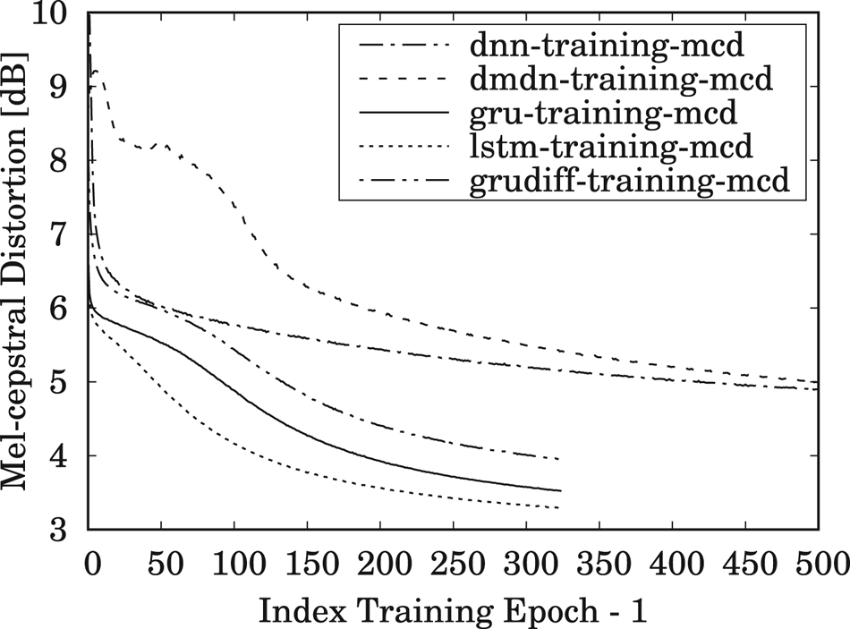
Fig. 5. Trend of mel-cepstral distortion (MCD) for the training set using the DNN-, DMDN-, LSTM-, GRU-, and GRUDiff-based spectral conversion models during 500 training epochs for the DNN/DMDN models and 325 training epochs for the LSTM/GRU/GRUDiff models.

Fig. 6. Trend of MCD for the testing set using the DNN-, DMDN-, LSTM-, GRU-, and GRUDiff-based spectral conversion models during 500 training epochs for the DNN/DMDN models and 325 training epochs for the LSTM/GRU/GRUDiff models.
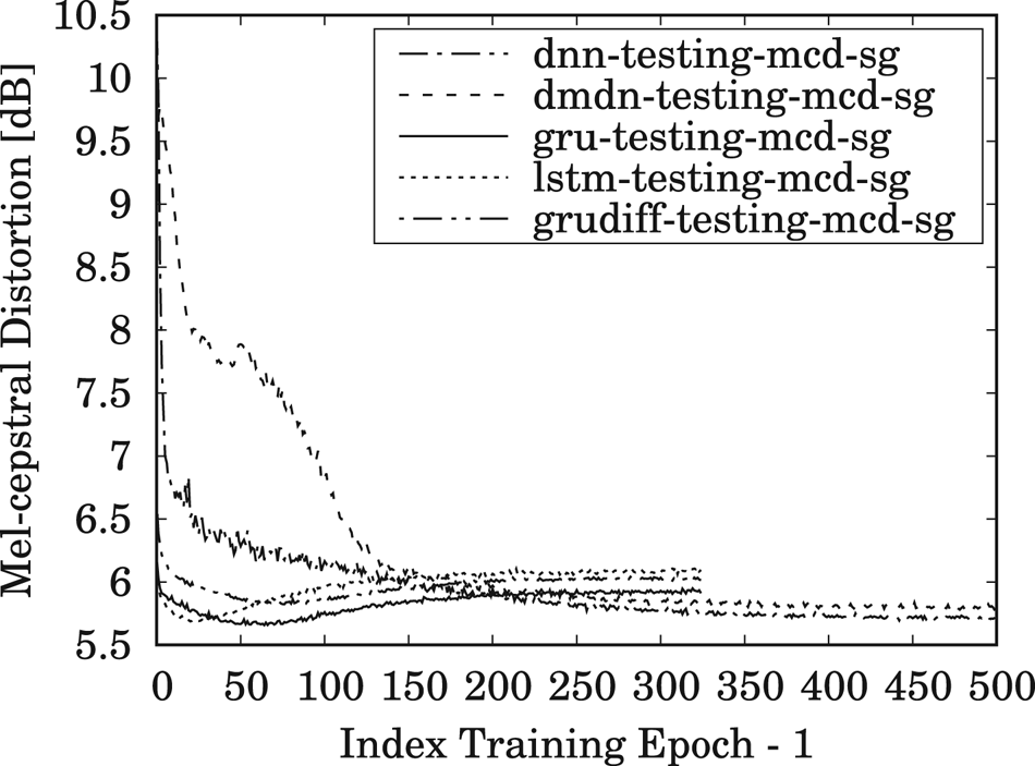
Fig. 7. Trend of MCD for same-gender (SG) conversions on the testing set using the DNN-, DMDN-, LSTM-, GRU-, and GRUDiff-based spectral conversion models during 500 training epochs for the DNN/DMDN models and 325 training epochs for the LSTM/GRU/GRUDiff models.
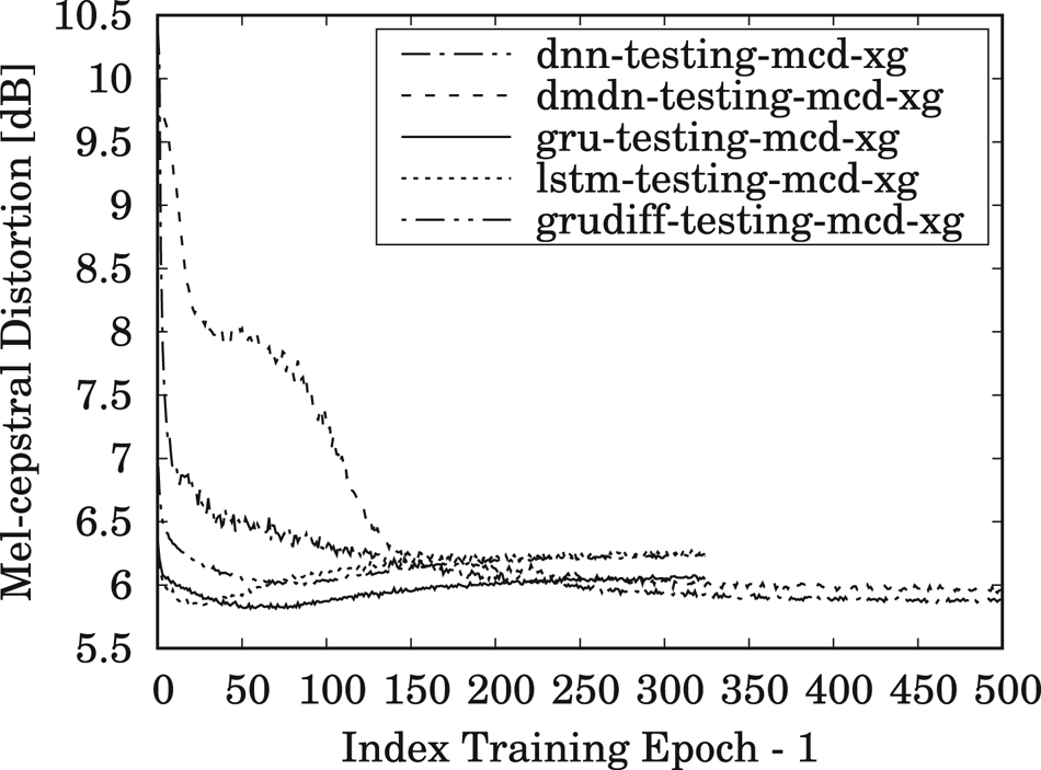
Fig. 8. Trend of MCD for cross-gender (XG) conversions on the testing set using the DNN-, DMDN-, LSTM-, GRU-, and GRUDiff-based spectral conversion models during 500 training epochs for the DNN/DMDN models and 325 training epochs for the LSTM/GRU/GRUDiff models.
Hence, to accompany the pure accuracy results of MCD, the LGD measurements were performed to evaluate the oversmoothness (variance reduction) of spectral trajectory due to the mean-based optimization in spectral modeling. The results of the LGD measurements of the testing data for same- and cross-gender conversions are given in Figs 9 and 10, respectively. These results demonstrate that the proposed spectrum differential loss used for the GRUDiff models makes it possible for the resulting converted trajectory to be less oversmoothed. Furthermore, all of the RNN-based spectral models show a clear tendency of being capable of producing better trajectory variance compared to the DNN-/DMDN-based models, such as the one used in our previous work [Reference Tobing, Wu, Hayashi, Kobayashi and Toda24], i.e. DMDN-based model. Considering the capability of GRU and GRUDiff to produce superior objective results, we used them both to generate converted spectra in the subjective evaluation. As to the latter point, in this work, we indeed focus on providing empirical evidence of the performance of RNN-based architectures for the VC framework, which would be beneficial for the continuous future development of real-world applications and integration of training development with other frameworks, such as neural vocoder.

Fig. 9. Trend of log-GV distance (LGD) for SG conversions on the testing set using the DNN-, DMDN-, LSTM-, GRU-, and GRUDiff-based spectral conversion models during 500 training epochs for the DNN/DMDN models and 325 training epochs for the LSTM/GRU/GRUDiff models.
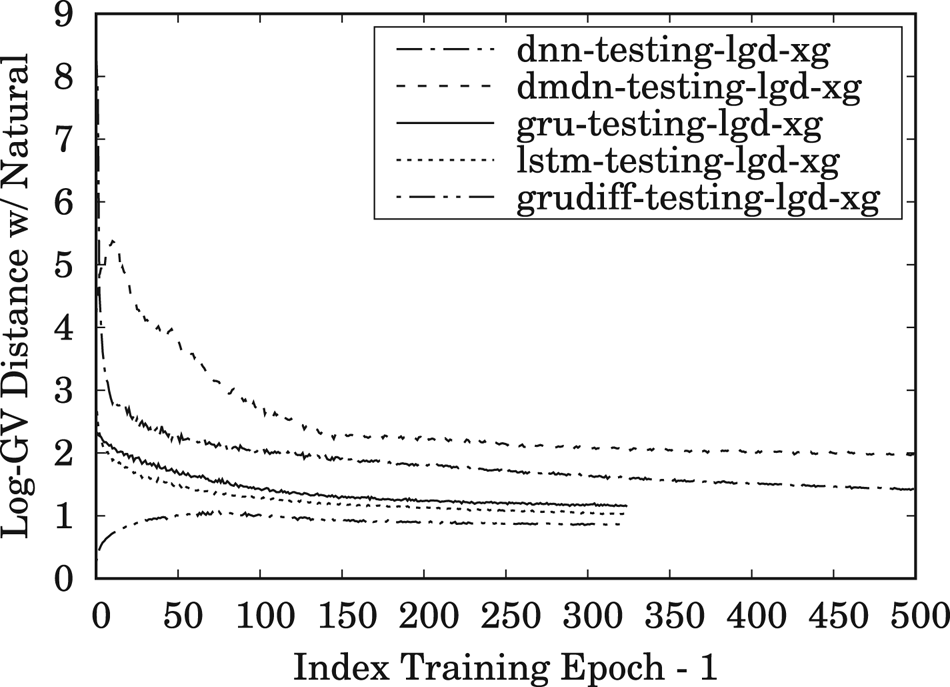
Fig. 10. Trend of LGD for XG conversions on the testing set using the DNN-, DMDN-, LSTM-, GRU-, and GRUDiff-based spectral conversion models during 500 training epochs for the DNN/DMDN models and 325 training epochs for the LSTM/GRU/GRUDiff models.
C) Subjective evaluation
In the subjective evaluation, we conducted MOS tests to evaluate the naturalness of the converted speech waveforms and speaker similarity tests to evaluate the accuracy of the converted speech waveforms. In the MOS tests, a five-scale score was used to assess the naturalness of speech utterances, i.e. 1: completely unnatural, 2: mostly unnatural, 3: equally natural and unnatural, 4: mostly natural, 5: completely natural. On the other hand, for the speaker similarity tests, each listener was given a pair of stimuli, i.e. a natural speech of the target speaker and a converted speech of the source speaker, and asked to judge whether or not the two speech utterances were produced by the same speaker. To judge the similarity, each listener chose between two main responses, i.e. “same” or “different”, where each had a confidence measurement, i.e. “sure” or “not sure”, giving a total of four options when judging the similarity. The number of listeners was 10.
We compared the use of direct waveform modification with the spectrum differential, i.e. DiffVC [Reference Kobayashi, Toda and Nakamura5], using the GV [Reference Toda, Black and Tokuda22] postfilter (dG), which was made to nearly matching the baseline system of VCC 2018 [Reference Kobayashi and Toda68], and the use of the WN vocoder to generate the converted speech waveforms. In the case of the WN-based waveform generation, we also compared the use of several types of speech auxiliary features, namely, converted spectral features (WNc), converted features with the GV postfilter (WNcG), post-conversion processing based on DiffVC (WNd), and DiffVC post-conversion processing with the GV postfilter (WNdG), which was used for our VC system in VCC 2018 [Reference Tobing, Wu, Hayashi, Kobayashi and Toda24]. Furthermore, we also utilized two different spectral mapping models, i.e. the GRU-based models with conventional loss (GRU) and spectrum differential loss (GRUDiff). The total combinations of speaker pairs and spectral mapping models/waveform generation methods were 40, i.e. four speaker pairs and ten different models/methods. In the naturalness evaluation, the number of distinct utterances was three, whereas, in the speaker similarity evaluation, it was two. In both evaluations, we also included the original speech waveform of the four speakers, i.e. either as a single stimulus of the original waveform in naturalness test or a pair of stimuli of original waveforms (from either source–target/target–target) in similarity test. Therefore, each listener had to evaluate 132 audio samples in the naturalness test and 92 audio samples in the similarity test.
The results of the MOS tests are shown in Tables 1 and 2. It can be observed the DiffVC with the GV method yields relatively high naturalness scores for same-gender conversions but not for cross-gender conversions owing to the use of the conventional vocoder in the cross-gender conversions. On the other hand, for the WN-based waveform generation, the use of post-conversion processing based on DiffVC and the GV, i.e. WNdG, clearly enhances the naturalness of the converted speech waveforms compared with the other sets of auxiliary speech features. Furthermore, the proposed spectrum differential loss improves the performance for same-gender conversions, i.e. either F-to-F or M-to-M.
Table 1. Results of mean opinion score (MOS) test of DiffVC with the GV postfilter (dG) waveform generation method using either GRU or GRUDiff spectral mapping models and of the original speech signals.
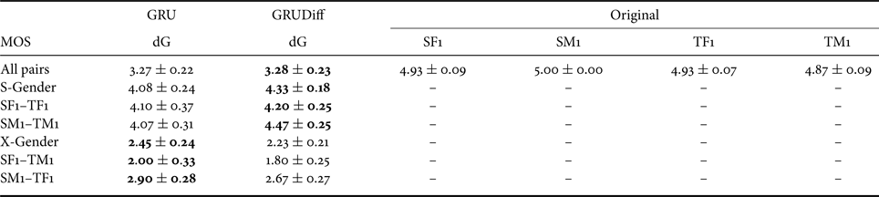
$\pm$ denotes the $95\%$
 confidence interval. S-Gender and X-Gender denote same-gender and cross-gender conversions, respectively.
Table 2. Results of MOS test of the WN-based generation methods using plain converted mel-cepstrum (c), using c with GV postfilter (cG), using post-conversion based on DiffVC (d), and using d with GV postfilter (dG) from either GRU or GRUDiff spectral mappings.
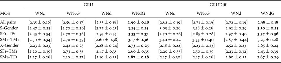
S-Gender and X-Gender, respectively, denote same-gender and cross-gender conversions. $\pm$ denotes the $95\%$
 confidence interval of the sample mean. Bold indicates the system(s) with the highest mean score in each conversion category. [$\cdot$
 ] Denotes a system with a statistically significant lower score than the highest score in each conversion category. Statistical inferences were performed using the two-tailed Mann–Whitney test with $\alpha <0.05$
 .
.
Results for the speaker similarity tests are given in Table 3. The results show that the use of the WN vocoder with the DiffGV-based post-conversion processed auxiliary features (WNdG) yields superior accuracy to the other methods, including the conventional DiffGV without the WN vocoder (dG). The results for naturalness and accuracy in this paper exhibit a similar tendency to the results of VCC 2018 [Reference Lorenzo-Trueba51], where the baseline method [Reference Kobayashi and Toda68] yields better naturalness, especially for same-gender conversions, due to the avoidance of the conventional vocoder, and our VC system with post-conversion processing for the WN vocoder [Reference Tobing, Wu, Hayashi, Kobayashi and Toda24] gives better accuracy. Based on these results, for the use of a WN vocoder in VC, it has been shown that an additional processing procedure adjusted to reduce the mismatches between estimated and natural speech features is needed to improve the converted speech waveform. For future work, it is worthwhile to directly address this problem in the development of a neural vocoder, such as WN, for VC, i.e. in a data-driven manner. All audio samples used in the subjective evaluation are available at http://bit.ly/2WjuJd1.
Table 3. Results of speaker similarity test (scores were aggregations of “same – sure” and “same – not sure” decisions) of the converted speech waveform using all waveform generation methods (dG, WNc, WNcG, WNd, and WNdG) with either GRU or GRUDiff spectral mappings.
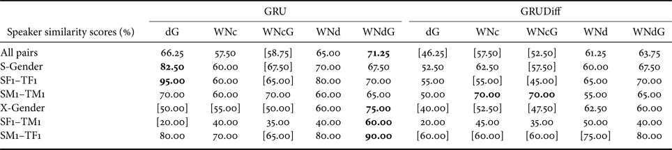
S-Gender and X-Gender, respectively, denotes same-gender and cross-gender conversions. Bold indicates the system(s) with the best similarity score in each conversion category. [$\cdot$ ] Denotes a system with a statistically significant lower score than the best score in each conversion category. Statistical inferences were performed using the two-tailed Mann–Whitney test with $\alpha <0.05$
 .
.
VI. CONCLUSION
In this paper, we have presented a study on the use of NN-based statistical models for both spectral mapping and waveform generation in a parallel VC system. Several architectures of NN-based spectral mapping models are presented, including DNN-, DMDN-, and RNN-based architectures, i.e. by using LSTM/GRU units. Then, we have presented the use of WN vocoder as a state-of-the-art NN-based waveform generator (neural vocoder) for VC. The problem of quality degradation faced by the WN vocoder in VC owing to the oversmoothed characteristics of the estimated parameters is handled through post-conversion processing based on the direct waveform modification with spectrum differential (DiffVC) and the GV post-filter, i.e. DiffGV. Furthermore, to preserve the consistency with the DiffGV-based post-conversion method, we have proposed a modified loss function that minimizes the spectrum differential loss for the spectral modeling. The experimental results have demonstrated that: (1) the RNN-based spectral modeling, particularly the GRU-based model, achieves higher spectral mapping accuracy with a faster convergence rate and better generalization than the DNN-/DMDN-based models; (2) the RNN-based spectral modeling is also capable of generating less oversmoothed spectral trajectory than the DNN-/DMDN-based models; (3) the use of spectrum differential loss for the spectral modeling further improves the performance in same-gender conversions; and (4) the DiffGV-based post-conversion processing for the converted auxiliary speech features used in the WN vocoder achieves superior performance for both naturalness and speaker conversion accuracy compared to those obtained using conventional sets of converted auxiliary speech features. Future work includes the use of a GRU-based model for non-parallel VC and to directly address the mismatches of speech features for VC with the neural vocoder in a data-driven manner.
FINANCIAL SUPPORT
This work was partly supported by the Japan Science and Technology Agency (JST), Precursory Research for Embryonic Science and Technology (PRESTO) (grant number JPMJPR1657); JST, CREST (grant number JPMJCR19A3); and Japan Society for the Promotion of Science Grants-in-Aid for Scientific Research (KAKENHI) (grant numbers JP17H06101 and 17H01763).
STATEMENT OF INTEREST
None.
Patrick Lumban Tobing received his B.E. degree from Bandung Institute of Technology (ITB), Indonesia, in 2014 and his M.E. degree from Nara Institute of Science and Technology (NAIST), Japan, in 2016. He received his Ph.D. degree in information science from the Graduate School of Information Science, Nagoya University, Japan, in 2020, and is currently working as a Postdoctoral Researcher. He received the Best Student Presentation Award from the Acoustical Society of Japan (ASJ). He is a member of IEEE, ISCA, and ASJ.
Yi-Chiao Wu received his B.S and M.S degrees in engineering from the School of Communication Engineering of National Chiao Tung University in 2009 and 2011, respectively. He worked at Realtek, ASUS, and Academia Sinica for 5 years. Currently, he is pursuing his Ph.D. degree at the Graduate School of Informatics, Nagoya University. His research topics focus on speech generation applications based on machine learning methods, such as voice conversion and speech enhancement.
Tomoki Hayashi received his B.E. degree in engineering and his M.E. and Ph.D. degrees in information science from Nagoya University, Nagoya, Japan, in 2013, 2015, and 2019, respectively. He is currently working as a Postdoctoral Researcher at Nagoya University. His research interests include statistical speech and audio signal processing. He received the Acoustical Society of Japan (ASJ) 2014 Student Presentation Award. He is a member of IEEE and ASJ.
Kazuhiro Kobayashi received his B.E. degree from the Department of Electrical and Electronic Engineering, Faculty of Engineering Science, Kansai University, Japan, in 2012, and his M.E. and Ph.D. degrees from Nara Institute of Science and Technology (NAIST), Japan, in 2014 and 2017, respectively. He is currently working as a Postdoctoral Researcher at the Graduate School of Information Science, Nagoya University, Japan. He has received a few awards including the Best Presentation Award from the Acoustical Society of Japan (ASJ). He is a member of IEEE, ISCA, and ASJ.
Tomoki Toda received his B.E. degree from Nagoya University, Japan, in 1999 and his M.E. and D.E. degrees from Nara Institute of Science and Technology (NAIST), Japan, in 2001 and 2003, respectively. He was a Research Fellow of the Japan Society for the Promotion of Science from 2003 to 2005. He was then an Assistant Professor (2005–2011) and an Associate Professor (2011–2015) at NAIST. Since 2015, he has been a Professor in the Information Technology Center at Nagoya University. His research interests include statistical approaches to speech and audio processing. He has received more than 10 paper/achievement awards including the IEEE SPS 2009 Young Author Best Paper Award and the 2013 EURASIP-ISCA Best Paper Award (Speech Communication Journal).


 Open access