


1. Introduction
Both economists and demographers examine the balance between economic and non-economic factors in orchestrating a fertility transition, as witnessed in historical European populations and in some East Asian economies over relatively short periods of time. Classic studies of fertility such as the Princeton Fertility Project highlight that the transition to low fertility in historical European populations occurred in a variety of socio-economic and institutional contexts, with a significant role being played by the local social environment [Coale and Watkins (Reference Coale and Watkins1986), Federici et al. (Reference Federici, Mason and Sogner1993)]. More recent studies have emphasized the role of the social climate and the influence of social interactions on demographic behavior [Manski and Mayshar (Reference Manski and Mayshar2003), Munshi and Myaux (Reference Munshi and Myaux2006)]. These empirical findings have led many economists to focus on modeling the influence of social interactions on contemporary fertility transitions [Durlauf and Walker (Reference Durlauf and Walker1999), Manski and Mayshar (Reference Manski and Mayshar2002)] and on the reproductive externalities and coordination failures associated with fertility behavior per se [Dasgupta (Reference Dasgupta2000), Kohler (Reference Kohler2001), Iyer and Velu (Reference Iyer and Velu2006)].
The total fertility rate in Kenya fell from an average of 6 births per woman in 1948 [Ajayi and Kekovole (Reference Ajayi, Kekovole and Jain1998)] to approximately 4.56 in 2010 [CIA (2010)]. However, the most significant declines in fertility occurred over a 20-year period: the Demographic and Health Survey (DHS) studies conducted in 1989, 1993, and 1998 showed that the total fertility rate (TFR) dropped from 6.7 in 1989 and 5.4 in 1993 to 4.7 in 1998. This drop in fertility is considered one of the most dramatic recorded anywhere in the developed and developing world [Ajayi and Kekovole (Reference Ajayi, Kekovole and Jain1998), p. 116]. So it is useful to examine how fertility declined in this society. Moreover, our focus on ethnicity and fertility in Kenya mirrors policy discussions in Kenya that surrounded the release of the controversial Kenya Census figures in 2010 which included ethnicity and tribal affiliations for the first time, following the ethnic tensions of 2007–2008. In light of the sensitivity of these issues, we focus our study of ethnicity, religion, and fertility on an earlier period in Kenya's demographic history.
Our focus on religion and fertility is motivated by a wider demographic literature that has argued that this issue needs further investigation in developing country contexts [Iyer (Reference Iyer2002a, Reference Iyer2002b), Iyer (Reference Iyer, Carvalho, Iyer and Rubin2019)]. In a broad context, fertility is higher across the world for Muslims than for Christians [Iyer (Reference Iyer, Carvalho, Iyer and Rubin2019)]. This paper presents a context where both Muslims and Christians co-exist, but there are also ethnic differences which may swamp the religious differences. Kenya is a country which displays a great deal of heterogeneity by ethnicity but also by religion. In fact, it is a very interesting example of a society in which religion and ethnicity have interacted to influence the behaviors. While ethnic groups have predated the influence of religions like Christianity and Islam in Kenya, there are also indigenous religions here which are less common now, but which predate Christianity and Islam. Hence it is quite useful also to examine how historically well-defined social groups, whether delineated by religion or ethnicity, or both, interact with each other to influence the outcomes such as demographic behavior.
Economists consider the impact of social interactions within predetermined groups [Akerlof (Reference Akerlof1997), Brock and Durlauf (Reference Brock, Durlauf, Heckman and Learner2000), Brock and Durlauf (Reference Brock and Durlauf2001)], and how group formation results from social interactions with particular emphasis on residential neighborhoods, geographic proximity, and dynamic group formation [Borjas (Reference Borjas1995), Ginther et al. (Reference Ginther, Haverman and Wolfe2000), Conley and Topa (Reference Conley and Topa2002)]. Our study examines the social interactions in predetermined groups in Kenya such as religious groups and ethnic groups that are motivated by the anthropological literature on Kenya. Important previous studies which have examined the fertility rates and education in Africa have highlighted the significance of social interactions in Kenya [Behrman et al. (Reference Behrman, Kohler and Cotts-Watkins2002), Kravdal (Reference Kravdal2002), Rutenberg and Cotts-Watkins (Reference Rutenberg and Cotts-Watkins1997)].
In line with these studies, we conceive of the fertility of a Kenyan woman to be influenced by a range of factors such as her individual characteristics and the characteristics of the household to which she belongs. However, we also take these studies forward by suggesting that the social environment impinges on a woman's behavior by multiple interactions both at the household level and at the level of other reference groups such as religion and ethnicity. We highlight a crucial point often overlooked in the theoretical and empirical literature on this issue: namely that there are different levels at which social interactions occur. In doing so, we consider the possibility that both local and global forms of social interaction may coexist [Horst and Scheinkman (Reference Horst and Scheinkman2003)]. We quantify the effects of social interactions and group membership on the number of children ever born (CEB), highlighting whether these effects are mediated through household composition, ethnic affiliation, religion, a neighborhood cluster effect, timing effects, or some combination thereof.
In section 2, we provide an overview of ethnic and religious groups in Kenya, highlighting the characteristics which are relevant for fertility behavior. Section 3 summarizes social interactions and fertility behavior including theory, measurement, and estimation. Section 4 presents our demographic data. Section 5 discusses how we use unique district-level rainfall data from Kenya's meteorological rainfall stations over time to identify the variations in fertility by ethnic group. We discuss our results in section 6, and section 7 concludes.
2. Anthropological overview of groups in Kenya
Social interactions and channels of message transmission about fertility behavior are important at the level of ethnicity. Members of different ethnic groups speak the same language, usually adopt similar cultural practices, and with some exceptions in border areas, reside closely in the same, or in contiguous districts [Fapohunda and Poukouta (Reference Fapohunda and Poukouta1997)]. In the specific case of Kenya, it has been argued that cultural norms may encourage high fertility but also contribute to fertility decline over time [Caldwell and Caldwell (Reference Caldwell and Caldwell1987), Ascadi et al. (Reference Ascadi, Ascadi, Bulatao, Ascadi, Ascadi and Bulatao1990)]. We argue that individuals' multiple levels of social interactions reflect their social identities—regional identities, ethnic identities, religious identities, linguistic identities. While we do not explore the question of identity in this paper, we do focus on how local and global interactions that arise from these identities significantly affect individuals' behavior. Our analysis is based upon historical and anthropological studies of Kenya with particular focus on the features of Kenya's major ethnic and religious groups that have relevance for fertility behavior. In this section, we discuss the groups with reference to their population composition, the region of their residence, and three characteristics of these groups which are noteworthy—their residential pattern of settlement, clan organization, and education. These characteristics have implications for the politics of fertility in Kenya.
2.1 Population
The population of Kenya consists of three groups—the Africans, and to a lesser extent, the Asians, and Europeans. Although the last two groups mainly reside in towns, 90% of the African population continues to live in rural areas [see Meck (Reference Meck1971)]. The tribal groups of rural Kenya live in clearly defined settlements in the more remote areas. In the Lake Victoria basin, the highlands, and the coast, there is a more heterogeneous population structure [Morgan and Shaffer (Reference Morgan and Shaffer1966), p. 2, Meck (Reference Meck1971), p. 24]. The tribes can be defined broadly into four groups as classified by their language: the Bantu, the Nilotic, the Nilo-Hamitic, and the Hamitic. Within these four broad language groups, ethnic groups represent an additional sub-division. According to the original 1969 Population Census, there are 42 different ethnic African groups in Kenya [Rep (1970)]. According to the most recent 2009 Census, the five largest groups, accounting for over 75% of the population, are the Kikuyu (17%), Kamba (10%), Kalenjin (13%), Luhya (14%), and Luo (10%) [CIA (2010)]. Their population, according to recent controversial Kenyan census is the Kikuyu at 6.6 million, the Luhya at 5.3 million, the Kalenjin at 4.9 million, the Luo at 4 million, and the Kamba at 3.8 million (Kenya National Bureau of Statistics). There are also smaller groups such as the Mijikenda (5%), Meru (4%), Turkana (2.5%), Maasai (2.1%). About 9% of the population are smaller indigenous group below 1% each, and the Arabs, Indians, and Europeans are about 1%.
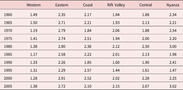
The Kenyan population is 41 million in total in 2011, growing at an average growth rate of more than 3% per year from 1980 to 2010 and at 2.7% CIA (2010). These Census data from Kenya thus depict a steady increase in the total population of Kenya from 1948 to the present. The total fertility rate in Kenya has fallen from an average of 6 births per woman in 1948 [Ajayi and Kekovole (Reference Ajayi, Kekovole and Jain1998)] to approximately 4.56 in 2010 [CIA (2010)]. However, the most significant declines in fertility have occurred in the last 20 years: the DHS studies conducted in 1989, 1993, and 1998 showed that the TFR dropped from 6.7 in 1989 and 5.4 in 1993 to 4.7 in 1998. This drop in fertility is considered one of the most dramatic recorded anywhere in the developed and developing world [Ajayi and Kekovole (Reference Ajayi, Kekovole and Jain1998), p. 116]. The fertility differences by ethnic group are also very large, as shown in Table 1. For women aged 15–49, the mean CEB varies from 2.5 for the Kikuyu to 3.5 for the Luo. Previous studies of fertility and ethnicity in Kenya have revealed that desired family size is smaller among the Kamba, Kikuyu, Luhya compared to the Luo [Fapohunda and Poukouta (Reference Fapohunda and Poukouta1997)]. The Luo exhibit a strong preference for large families (although this could also be driven by lower costs of children) and it is reported to use contraception much less than other groups [Watkins et al. (Reference Watkins, Rutenberg and Green1995)].
Table 1. Children ever born by region and ethnicity

$\mu _{{\rm ceb}}^E$ ($\mu _{{\rm ceb}}^R$
 ) denote, respectively, mean of CEB by ethnicity (region).
− denotes a zero sample count.
2.2 Religion
The predominant religion in Kenya is Christianity [Pew (2019)]. In 2019, an estimated 84.8% of the total population of Kenya is Christian. Islam is the second largest religion in Kenya, and practiced by 11.1% of the population. Other religious faiths observed in Kenya today are the Baha'i faith, Buddhism, Hinduism, and various traditional religions. Roman Catholicism first came to Kenya in the 15th century with the advent of the Portuguese, and then spread rapidly during the 20th century due to missionary activity. Today, the main Christian denominations in Kenya are Protestant and they comprise about 47.4% of the country's religious population. The Roman Catholic Church is about 23.3% of the population. The non-Protestant and non-Catholic groups constitute approximately 11.8% of the population. Most Muslims in Kenya are Sunni Muslims. Traditional religions include the Kikuyu religion and the Mijikenda religion and there are also the Maasai, Turkana, Samburu, and Pokot tribes who adhere to traditional religions. The number of Hindus in Kenya is small and only about 0.14% of the population. In our DHS sample, there are three main religions which comprise 96.5% of household. The dominant religion is Protestant (66.2%), followed by Catholic (27.8%) and Muslim (2.5%). A total of 3.2% of households report no religious faith. A religious breakdown of the ethnic groups shows that most Kikuyu are Christians, probably because they were the Kenyan tribe with the closest links with Christian missions historically [Meck (Reference Meck1971), p. 27]. Over 90% of Luhya and Luo are Christians, compared to over 60% of Kamba. Some of the Mijikenda sub-groups, such as the Digo, are Muslim. In Tables 8–10 presented later in this paper, we examine the influence of social interactions with respect to ethnicity, also controlling for the effects of religion. As our results show later in the paper, despite these significant religious variations, religion does not matter as much as ethnicity in these contexts. We speculate that this may largely be because the ethnic identities predate the advent of Christianity and Islam in this society.
2.3 Region
Ethnic boundaries in Kenya, to a very large extent, are coterminous with political and administrative boundaries [Fapohunda and Poukouta (Reference Fapohunda and Poukouta1997)]. Today, the regional breakdown of the different ethnic groups is as follows: the Kalenjin reside in the Rift Valley; the Kikuyu live in the Central region, but have also migrated to Nairobi and the Rift Valley. The Meru/Embu reside in the North and East. The Luhya live in the Western province, but have also migrated to Nairobi and Mombasa. The Luo live in Nyanza, with Kisumu as their capital, but have also migrated to the Rift Valley. The Kamba live in close proximity to Nairobi and exhibit ethnic affiliation to the Kikuyu. The Mijikenda/Swahili live in the Coast province. The Meru and Embu groups neighbor the Kikuyu to the north and east. An early study suggests that the Luhya, who live in Kenya's Western province, are a less homogenous group compared to the Kikuyu and Kamba [Were (Reference Were1967)]. Among the Luhya, there is a distinction that needs to be made between those in the north and those in areas such as Kakamega, with high population density. Although the Luo who live in Nyanza depict a rate of population growth almost as high as the Luhya, they are a more urbanized people [Ominde (Reference Ominde1968)]. For the Kamba, proximity to Nairobi and their close ethnic affiliation to the Kikuyu are particularly significant [Berg-Schlosser (Reference Berg-Schlosser1984)]. The Mijikenda and Swahili groups who reside in Kenya's Coast province are the most agricultural of all of Kenya ethnic groups.Footnote 1
2.4 Residential pattern of settlement
One of the most notable features of these ethnic groups is their pattern of residence.Footnote 2 It is important to emphasize that the notion of the “village” in this society is rather more diffuse than in the compact settlements of Europe and elsewhere. Although there are differences between ethnic groups, families are grouped mainly in homesteads that are located in clusters, and which form the basis of community interaction. In some of these clusters, for example, among the Kikuyu, there exist groups of households who are not merely coresident, but also related by blood and marriage. In other clusters, there are households that are located in close proximity, but where individuals in these households are not related to other individuals in neighboring households.
For example, the Kalenjin live mainly in homesteads that are individual family based. Property is usually inherited along paternal lines or male agnates. The smallest unit of territorial composition in Kalenjin society is the “temenik” or hamlet, a cluster of homesteads; these are usually grouped into “villages” of 15–60 temenik. The Kikuyu live in homesteads on land owned by the family, and surrounded by fields (or “shamba”). Traditionally, the land was owned by many households which constitute the extended family located on the same “ridge” which is the traditional geographical divisionFootnote 3 [Berg-Schlosser (Reference Berg-Schlosser1984), p. 50]. Supplementing the organization of Kikuyu society based on kinship, there is also a geographical demarcation. The “itura” or village consists of groups of families. This is further subdivided into those living on the same ridge. The pattern of Luo settlement is similar to other communities, although their homesteads usually consist of families who own land, dispersed as a safeguard against climatic conditions. The Kamba are also agriculturists, and their pattern of settlement is similar to the Kikuyu [Middleton and Kershaw (Reference Middleton and Kershaw1965)]. The traditional land-owning unit is the extended family. In terms of territorial residence, the most basic unit is the ukambani, which is a homestead that comprises several extended families. Several of these are grouped to form a kivalo within which social interactions, especially marriage, take place. For the Mijikenda, the main form of residence is the mudzi or village which consists of groups of agriculturists and fisherman.
2.5 Clan organization
These tribal groups are also broadly characterized by three main features that have relevance for social interactions: the importance of the family group, the clan, and the system of age-gradingFootnote 4 [Meck (Reference Meck1971)]. For example, anthropological studies of the agriculturalist Kikuyu argue that among them, fathers exert a less important role for economic decision-making, that relations between the extended family are strong, and that they exhibit a highly evolved sense of ethnic identity which can often override more national concerns [Berg-Schlosser (Reference Berg-Schlosser1984), Ferguson and Srung Boonmee (Reference Ferguson and Srung Boonmee2003)]. Anthropologists comment that among the Kikuyu, the most economically and socially effective unit is the mbari: “a group of families who trace their descent from a common ancestor following the paternal line, often for up to seven or eight generations. In addition to its functions as the most important traditional land-holding unit in Kikuyu society, the mbari is an important social reference-group for many Kikuyu and still plays an effective role in many economic and social relationships including the more modern ones” [Berg-Schlosser (Reference Berg-Schlosser1984), p. 53]. We would therefore expect that the endogenous social interaction effects among this group would emerge as being particularly strong. The Luhya do not have as powerful a clan organization as some of the other groups [Meck (Reference Meck1971), p. 28]. Anthropologists comment that a feature of the Luhya that makes them quite distinct from other groups is the relatively strict accepted norms of behavior, particularly with respect to marriage and interactions between the sexes [Berg-Schlosser (Reference Berg-Schlosser1984), p. 114].
2.6 Polygyny
One of the interesting features of African societies including Kenya is the incidence of polygyny. Polygyny can have two impacts on fertility: first, it can increase fertility if there is more help provided with child-care, creating a micro-level externality within the extended family household. Second, if there is a greater discussion of family planning issues, then this might work to reduce fertility. Alternatively, if high-fertility norms are espoused within the extended household, then the effect might be to increase fertility. A number of recent studies have examined the role of polygynous marriage norms in influencing demographic behavior [Hogan and Biratu (Reference Hogan and Biratu2004)]. There are 30% of polygynous households in the KDHS sample that we consider in this study, so these were households that had more than one wife living in the household. This is not related to the household's religious affiliation. The rationale for looking at polygyny is that if other household members help with child care, or indeed as with other African societies where “fosterage” is common, other residents have an important bearing on a woman's total fertility. A number of other demographic studies of poor societies [see, e.g., Iyer (Reference Iyer2002a, Reference Iyer2002b)] have found that the role played by residents within the household or within close proximity, such as friends and neighbors, is important for fertility. We acknowledge that the effects of polygyny might be even more complex than this. For example, unobserved differences among women who enter polygynist unions might be correlated with unobservables in the fertility equation. In general, the frequency of polygynous unions varies a great deal across Africa: DHS data show that they are between 30% and 50% in West Africa, 20% and 35% in East Africa, and less than 20% in Southern Africa. So our sample which has 30% polygynous unions is typical of East Africa where Kenya is situated geographically.
2.7 Mortality
Infant mortality and mortality caused by HIV/AIDS also would affect fertility rates. We examine infant mortality and the awareness of HIV/AIDS in the population, which are included in order to control for the fact that across all ethnic groups in Kenya, as like other countries in Africa, there has been a large increase in HIV-related deaths which might also affect fertility. For example, recent data show that 7.1–8.5% of adults aged 15–49 in Kenya are currently living with AIDS. Higher AIDS-related deaths may increase fertility if many children are lost to this. There is also the possibility of reverse causality in that low CEB groups may use contraceptive methods more and hence this is a cause of their low HIV rates as well. It is also important to examine infant mortality by ethnicity in Kenya. This is because demographers think that higher infant and child mortality is frequently associated with higher fertility rates if parents want to replace children who are lost to child death, or if they perceive that the average mortality rate in their region is high. So it is important to control for mortality changes which might also influence fertility in this country.
As regards to differences in mortality by ethnic groups in Kenya, Tabutin and Akoto (Reference Tabutin, Akoto, van de Walle, Pison and aSalad-Diakanda1992) found that the probability of infant mortality among the Luo was higher than among the Kikuyu. Brockerhoff and Hewett (Reference Brockerhoff and Hewett2000) argue that in Kenya, mortality differentials by ethnic group exist and are related to several factors. Migratory patterns influence the spread of disease, and economic and other conditions. For example, they contrast the Kalenjin who are more sedentary with the Luhya who migrate more and are hence more prone to exposure to infectious diseases. They also highlight the Kikuyu who have better access to health and education which meant that they first experienced initially at least the highest declines in mortality of any ethnic group in Kenya. For this reason, the Kikuyu also had very low child mortality (the under-5 mortality rate for Kikuyus was 36.1 per 1,000 live births in 1989–1993), but for non-Kikuyu groups, this was 125.1 deaths per 1,000 live births. They attribute this to resource concentration and high altitude that prevents the spread of malaria among Kikuyu children relative to other groups.
2.8 Education
Initiated first by Jomo Kenyatta, education policy in Kenya has been pursued actively by the government, with remarkable success, especially with increases in primary and secondary school enrolment for girls. However, despite the general increases in the uptake of education and policies such as school fee remission and the development of harambee or self-help community schools which foster these, the mean number of years of schooling differs considerably by ethnicity.
The mean number of years of education varies considerably by ethnic group in Kenya, as shown in Table 2. This factor has relevance for social interactions as we might expect the importance of social interactions on fertility to be mediated by the effect of education. Previous studies of Kenyan fertility argue that the Kikuyu and the Kamba show the least preference for large families because they had early access to colonial education [Fapohunda and Poukouta (Reference Fapohunda and Poukouta1997)]. The Kikuyu are the best educated, compared to other ethnic groups in Kenya [Berg-Schlosser (Reference Berg-Schlosser1984), p. 60, De Wilde (Reference De Wilde1967), p. 39]. We can explain this development historically—many Kikuyu worked as wage laborers in European-owned plantations and attended schools. As a community, they viewed education as the means to progress and this led them to acquire positions of responsibility in the colonial administration. In the post-Independence period, the Kikuyu continued to dominate and consolidate their position, politically and economically, relative to the other groups [Ferguson and Srung Boonmee (Reference Ferguson and Srung Boonmee2003)]. The Luhya populations are also highly literate groups. Most Kamba are enrolled in formal schooling. Among the Kalenjin, levels of education are, in general, less than other groups. The Mijikenda and Swahili groups also have low levels of education compared to other groups in this population.
Table 2. Mean education (years) by region and ethnicity
Note: $\mu _{{\rm ED}}^R$ $\lpar {\mu_{{\rm ED}}^E } \rpar$
 denotes mean years of education by region (ethnicity).
− denotes zero sample count.
2.9 Politics of ethnicity
Events in Kenya in 2007–2008 highlighted the importance of the politics of ethnicity in this country. Differences in the economic performance of ethnic groups can be traced to their evolution in Kenyan history and to economic decisions made by these groups [Ferguson and Srung Boonmee (Reference Ferguson and Srung Boonmee2003)]. Ethnic identity in Kenya has always been very strong historically, and it continues to be a very potent force in Kenya's politics even today. For example, the Kalenjin, who are a heterogeneous ethnic group and who live primarily in Kenya's Rift Valley province [Were (Reference Were1967)] are closest to Nairobi geographically, and they are politically and economically Kenya's dominant ethnic group [Kenyatta (Reference Kenyatta1966)]. Their location in the eastern Rift Valley allows them to enjoy a level of political proximity that, in part, determines their (relatively) superior economic status. Agricultural innovation first arose among the Kikuyu who also absorbed land reform more readily than other groups [Meck (Reference Meck1971), p. 27]. Historically, the Kikuyu were one of the first ethnic groups in Kenya to absorb European-style capitalism in the form of wage labor and participation in the monetary economy, so in contrast, for example, to the Maasai whom they neighbor, the Kikuyu's subsequent economic performance has been much better [Ferguson and Srung Boonmee (Reference Ferguson and Srung Boonmee2003)].Footnote 5 In the past, the Luo were less responsive to social and economic change compared to other tribes [Meck (Reference Meck1971)]. For example, land reform met with a great deal of resistance among this group as it was believed to conflict with religious beliefs. But since 2001, the Luo have increasingly been incorporated into the government. In more recent times, relations between the ethnic groups has been closely tied with the development of Kenyan politics, particularly since the introduction of multiparty politics in Kenya since 1991 after over 20 years of rule by one party [Throup (Reference Throup2001)]. The increased strength and importance of ethnic identity has also led, more worryingly, to ethnic clashes in 1992–93, 1997, and 2007–2008.
3. Social interactions and fertility: theory, measurement, and estimation
3.1 Theory
The conventional economic household demand model of fertility behavior posits that a couple's fertility is a function of the money costs of children and the opportunity costs of the value of parental time [Becker (Reference Becker1981)]. The standard Beckerian atomistic utility function [Becker (Reference Becker1981), Willis (Reference Willis1973)] is given by

where U i denotes the utility function of household i, c i represents the number of children, ${\bi z}_i$ is all sources of satisfaction to the husband and wife other than those arising from children, and ${\bi x}_i$
 denotes the vector of socio-demographic characteristics which affect preferences.Footnote 6 ɛi allows for imperfect information on the part of the analyst. This is subject to the usual budget constraint

where we assume that total income I i is expended on children c i and on all sources of satisfaction other than those arising from children, ${\bi z}_i$ ; p c and ${\bi p}_z$
 are the shadow prices of children and other sources of satisfaction, respectively.
The extension of the atomistic utility model to incorporate social interactions allows us to capture that component of individual utility attributable to a fertility choice c i that is dependent upon the fertility choices of others [see, e.g., Becker and Murphy (Reference Becker and Murphy2000)]. The “others” in question may be those resident in the individual's household or in the local community; for example, in the individual's street or neighborhood.
It is important to distinguish between local and global interactions as individual behavior may be determined by the decisions of a larger ethnic group. In a local interaction, individuals have incentives to conform to the behavior of a small number of appropriately defined neighbors, whose actions they can “observe”. In contrast, a global interaction is where individuals face incentives to conform to the “expected” behavior of a common reference group, whose behavior we cannot observe. It is possible that these expectations are channeled through the media, or through other norms of behavior such as knowledge of the customs and traditions of particular ethnicities. There is thus the possibility of multiple social interactions—namely that social interaction is both localized within a specific location, and more diffuse across a larger, geographically diffuse sub-population.
Following Manski (Reference Manski1993), three hypotheses are advanced to explain why individuals belonging to a common reference group behave similarly.Footnote 7 In a fertility context, there is an endogenous effect if, ceteris paribus, CEB to a woman varies with the average CEB of members of her ethnic group or locality, perhaps because she suffers a utility loss from deviations from group behavior.
There is an exogenous or contextual effect if, ceteris paribus, CEB to a woman varies with the average characteristics of her ethnic group or locality. For example, the existence of educated neighbors may foster positive attitudes toward smaller family size.
Education exercises a prominent effect on fertility behavior. For example, individual educational attainment affects individual-level fertility. In a developing society, this would be dependent on the money-costs of acquiring an education and the opportunity costs of wages foregone. There is also an iconic value of education as individuals may aspire to the attributes of other higher educated groups in a population. In some developing societies, the iconic value of education is very high. For example, sociologists of India comment on the phenomenon of “Sanskritization” in which lower-caste groups take on the characteristics and customs of the upper castes in order to gain greater legitimacy and status in the Indian social system. Frequently, this manifests itself in the desire to acquire an education or to continue one [Srinivas (Reference Srinivas1994)].
Finally, there is a correlated effect if, ceteris paribus, women in the same ethnic group or locality have similar CEB because they are, for example, similarly wealthy.
The importance of differentiating between these three hypotheses can be seen by examining their respective policy implications. Consider, for example, an intervention to provide free contraception to some members of an ethnic group or a number of neighborhoods. If there are endogenous effects, then an effective policy of free contraception may both directly reduce the fertility of the recipients but, as their fertility decreases, indirectly reduces the fertility of all other members of that ethnic group or neighborhood. Exogenous effects and correlated effects will not, in general, generate this kind of social multiplier effect.
3.2 Measurement
As outlined in section 2, using a number of anthropological sources, we have identified that within rural populations in Kenya, fertility decisions are conducted within families which are members of ethnic groups and/or religious groups, and which reside mainly in homesteads that are located in relatively small clusters. We postulate that these allegiances form the basis of social interactions. We focus on the role of two reference groups. First, an ethnicity effect derives from the fact that the status of women and attitudes toward children differ across ethnic groups, with a differential evaluation of the psychological costs and benefits of bearing children.Footnote 8
Second, in the case of Kenya, situated between the individual and the ethnic group, are small clusters of households within which physical proximity dictates that individuals directly observe and bear the costs of the decisions of others. The clusters are homogenous in that they usually consist of the same ethnic (and/or religious) group. In addition, we have information which allows us to distinguish between clusters which, for certain ethnic groups, are comprised of households which are blood-related, with obvious ramifications for interactions.Footnote 9 For example, in the case of the Kikuyu, we might expect the extent of such interaction to be on average higher given that clusters of households are generally comprised of groups of individuals which are related by blood and marriage (the mbari). In such a situation, one might expect to find a stronger normative influence relative to clusters comprised of households, as in the case of the Kalenjin, who live mainly in homesteads that are individual family based.
3.3 Estimation
In motivating a modeling strategy, we first consider the observed data. For each i th woman we observe $\lcub {c_i\comma \;{\bi x}_i\comma \;L_{ij}} \rcub \comma \;$ where c i represents a count of the total number of CEB, ${\bi x}_i$
 is a vector which includes individual characteristics, together with ethnic, cluster, and household attributes; L ij, j = 1, …, J denotes the j th location in which i resides.
Our sample, restricted to women between 30 and 49 years of age, is designed to capture the decision-making of women who have completed their fertility, thereby excluding relatively young women for whom timing effects may be confounded with changes in fertility. The presence of timing effects, for example, younger cohorts marrying at later ages, is important in that they determine, in part, the difference between the observed number of children for a given woman and the mean number of children in the appropriate reference group. This is central to our thesis, namely that changes in this difference will impact upon CEB due to an interaction effect.
Dynamic models of fertility consider birth spacing, birth timing, the influence of uncertainty, and essentially view fertility decisions sequentially [for a more recent example, see Iyer and Velu (Reference Iyer and Velu2006)]. Seminal dynamic models of fertility such as Wolpin (Reference Wolpin1984), Newman (Reference Newman1988), and Rosenzweig and Schultz (Reference Rosenzweig and Schultz1985) address questions such as the importance of birth timing and spacing. The Wolpin model examines birth spacing, birth timing, and intertemporal tradeoffs. In this model, an individual maximizes the expected value of the discounted sum of period utility over their lifetime by choosing a sequence of births and consumption, subject to infant mortality and shocks to household income.
3.3.1 Model specification
In this section, we consider the specification of the conditional mean, and in particular, the specification of the exogenous and endogenous components of fertility behavior.
Given that count data are both integer-valued and heteroscedastic by construction, the Poisson density represents a natural benchmark to model count data. However, the equidispersion property, namely that the conditional mean is equal to the conditional variance, is generally restrictive. In this paper, we utilize the Generalized Method of Moments (GMM) estimator. A GMM estimatorFootnote 10 is particularly suited given that it allows for unobserved heterogeneity without a full set of parametric assumptions, and readily accommodates endogenous regressors.
We write the conditional mean as

c i denotes the number of children (CEB) ever born to the i th woman. Equation (3) includes the standard set of individual (${\bi q}_i$ ), household (${\bi h}_i$
 ), and cluster (${\bi p}_g$
 ) characteristics, with associated vectors of parameters η, θ, and κ. cfig represents conformist interaction effects attributable to the fertility choices of other women in the same group. edg denotes exogenous interaction effects due to education which we measure by the mean level of education in the cluster resided by the individual. δ and γ are the associated scalar parameters.
Exogenous interaction effects. We represent exogenous effects attributable to the education of other women in the same cluster using ${\rm e}{\rm d}_g = N_g^{{-}1} \sum\nolimits_{i\in g}^{} {{\rm e}{\rm d}_i}$ with edi denoting the education level of the i th woman residing in the same cluster. It is argued that the effect of education is iconic, with some individuals aspiring to the attributes of other higher educated members within their cluster. We choose to model these education interactions at the level of the cluster as higher educated women in the locality may be leaders and opinion-makers who influence others who are less educated to adopt low fertility norms. Here we consider the proportion of women in the cluster who had completed higher education as representative of this exogenous education effect on fertility.
Endogenous interaction effects. We extend the standard atomistic utility model of fertility to capture that component of individual utility attributable to a fertility choice that is dependent upon the fertility choices of others. Individuals may have incentives to conform to the behavior of a small number of appropriately defined neighbors whose attributes they can “observe”.
In the conditional mean specification (3), endogenous conformist effects are represented by cfg = E i(c g − c i), where c i denotes the number of children (CEB) ever born to the i th woman, and E i(c g) is the subjective expectation of mean CEB held by the i th woman resident in cluster g.Footnote 11 Restricting the sample to those women aged 30–49 and thereby confining our analysis to completed lifetimes circumvents the problem of pooling data over age cohorts. For older women, we can appeal to rational expectations and set the subjective expectation of cohort fertility equal to the mean observed level of fertility, $E_i\lpar {c_g} \rpar = \bar{c}_g$ . However, this becomes problematic when considering subjective expectations of younger women who are not near the end of their reproductive careers.
In Appendix C, we outline our identification strategy which explains how we isolate the effect of social interactions from other determinants of fertility behavior. We do this by first outlining the identification problem in the linear-in-means social interaction model as originally considered by Manski (Reference Manski1993), and more recently by Blume et al. (Reference Blume, Brock, Durlauf, Ioannides, Benhabib, Jackson and Bisin2010) and Ioannides (Reference Ioannides, Blume and Durlauf2008). Since the question of identification is well understood in the linear framework, this will provide a useful point of departure.
3.3.2 Household-level and individual-level controls
We control for a number of household and individual characteristics that we believe impact fertility decisions to ensure that the endogenous and exogenous effects are robust to variations in other characteristics.
Individual-level controls. Individual-level controls include the age of the woman measured in years and an age-squared variable accounting for the non-linearity associated with age-related variables. The education of the woman is included and measured as the highest level of education attained, differentiating between primary, secondary, and higher education effects. The influence of the media was measured as whether the woman listened to the radio at least once a week. This variable was included on the assumption that greater information about contraceptive technology would be available to the woman if she listened to the radio. Messages about this are routinely broadcast on the national radio channel, the “Voice of Kenya” in English, Swahili, and the vernacular. We also include a variable here for whether the individual knows a place to test for HIV/AIDS. This is to control for their awareness of AIDS, which is an important contributor to mortality in Kenya and which therefore is likely to affect fertility, as also discussed in section 2.
We also include the following measures: age at first marriage and knowledge of any method of contraception. We expect that this will capture the extent to which the age at first marriage is greater for younger relative to older women. With the success of recent family planning programs in Africa, knowledge of contraception is also likely to be greater for younger women than older ones. We also control explicitly for the religion of the respondent.
Household-level controls. One notable problem with the DHS is that there are no direct questions on income were asked of survey respondents. Utilizing a series of questions asked about household quality, access to infrastructure, and the ownership of consumer durables, we constructed a number of indicators which control for the economic status of households. The quality of roof construction was measured by whether the household had a tiled roof or not. The quality of the floor was measured by whether the household had a tiled or wood floor or not. The status of the household was also proxied by the ownership of consumer durables including whether or not the household owns a radio, or a television.
Two other important household-level attributes that we utilized are (i) a measure of infant mortality, and (ii) reported awareness of HIV/AIDS in the population. These factors are included in order to control for the fact that Kenya has witnessed a large increase in HIV-related deaths over the time period under study which might also affect fertility; and that different religious groups might have different norms about contraception which can again affect both CEB and CEB rates. The DHS data provide data on infant mortality but because they do not have exact numbers for the HIV/AIDS-related deaths, we use reported awareness of HIV/AIDS in the population for our measure of how pervasive this is likely to be by region.
As discussed earlier, polygyny can have two impacts on fertility: first, it can increase fertility if within polygynyst households provide more child-care, creating a micro-level externality within the extended family household. Second, if there is a greater discussion of family planning issues, then this might work to reduce fertility. Alternatively, if high-fertility norms are espoused within the extended household, then the effect might be to increase fertility, again which might also be related to religion. There are 30% of households in the Kenya sample which are polygynous, so these were households that had more than one wife living in the household. We acknowledge that the effects of polygyny might be even more complex than this. For example, the coefficients on all other estimated parameters may vary by family structure. Unobserved differences among women who enter polygynist unions might be correlated with unobservables in the fertility equation. But we prefer to adopt a more parsimonious specification controlling for these effects. In order to do so, we also control for the number of usual residents in the household as a proxy for polygynous households.
3.3.3 Cluster attributes
We control for a number of attributes at the level of the cluster. Critical in this respect is access to water and fuel infrastructure. Based upon the work of Dasgupta (Reference Dasgupta2000), better access to water and fuel reduces the demand for child labor to collect them, and that this in turn reduces the demand for children, and hence the fertility rate [Iyer (Reference Iyer2002a, Reference Iyer2002b)]. Access to fuel was measured by a mean-level effect for access to electricity. Access to water infrastructure at the cluster-level was measured according to whether access to water was piped into the residence or not. In addition, an additional cluster-level attribute included was whether or not a radio was listened to at least once a week. This variable was estimated at the cluster level by aggregating up whether or not an individual listened to a radio. Finally, since the process of interaction will depend upon the size of the group, we control for the population size of the cluster.
4. Data and characteristics of the DHS survey
Our sample, taken from the Kenyan Demographic and Health Survey (KDHS), covers 88% of the population. The survey contains interview data for 7800 women aged 15–49. It contains women from all of Kenya's large ethnic and religious groups and covers a wide geographical area, omitting only the areas of extremely low population density in the North. Geographically, Kenya is divided into 7 provinces which are further subdivided into 47 districts. The KDHS covered 42 of Kenya's districts; 35 were sampled, 7 were not. Seventeen districts were oversampled. The representation of each group in the sample is similar to its representation in the whole population. The DHS data include information on ethnic groups, of which the six main groups are the Kikuyu, Kalenjin, Luhya, Luo, Kamba, and Kisii. The Kikuyu is the largest, with 17.9% of the population.Footnote 12 In the data used in this study, we consider individual-level data only for the 5,994 women residing in a rural cluster, and who did respond. The largest number of women included in the sample live in the Rift Valley region, while the smallest number of women sampled live in Nairobi.Footnote 13
The KDHS adopted a two-stage stratified sampling approach that selected households located within primary sampling units or sampling clusters. These clusters are identical to the complete enumeration of sample clusters which took place as part of the 1977 National Demographic Survey. The sample points themselves are identical to those chosen in the sampling frame maintained by the Kenyan Central Bureau of Statistics.
In the 35 of Kenya's 42 districts that were included in the survey, there were 536 clusters—444 rural clusters and 92 urban clusters, of which 530 were non-empty clusters.Footnote 14 The location of the clusters geographically is identifiable within the district and province [DHS and Macro International (1999), pp. 179–182]. A complete list of all households in each cluster was recorded between November 1997 and February 1998. From the remaining 530 clusters, a systematic sample was drawn of, on average, 22 households in urban clusters and 17 households in rural clusters. This formed a total of 9465 households. In these households, all women aged 15–49 were targeted for interview. Response rates varied by province from approximately 88% to 99% [for more details, see KDHS (1998), p. 180].
Table 1 presents the mean CEB by region and ethnicity. Average CEB varies from a low of 2.58 in Central to a high of 3.9 in Nyanza. For a number of regions, including Nyanza and Western, we observe notable intra-regional variation in CEB by ethnicity.
According to the DHS data, a rural woman has on average about 5.2 children compared to fertility among urban women at 3.1 children. Fertility differentials by the level of education show that illiterate women bear on average 5.8 children compared to 3.5 children for women with secondary school education [DHS (1998), p. xvii]. The sample reveals demographic differences between ethnic groups: for women aged 40–49, the mean CEB varies from 5.91 for Kikuyu to 7.56 for Luo. As shown in Table 1, the differences in fertility by ethnic group are clearly very large.
Our sample also records the religion of the household. There are three main religions which comprise 96.5% of household. The dominant religion is Protestant (66.2%), followed by Catholic (27.8%) and Muslim (2.5%). A total of 3.2% of households report no religious faith.Footnote 15 Table 3 presents the mean CEB by region and religion. The data reveal variation in mean CEB induced by the combination of religious and regional effects.
Table 3. Children ever born by region and religion
Note: Christian refers to all non-Catholics.
$\mu _{{\rm ceb}}^{Re}$ ($\mu _{{\rm ceb}}^R$
 ) denote, respectively, mean of CEB by religion (region)
− denotes a zero sample count.
The DHS data show that knowledge of family planning in Kenya is very high: 98% of women and 99% of men were able to name at least one modern method of contraception. There are 38% of women who use contraception and the most widely used methods are contraceptive injectables, the pill, female sterilization, and periodic abstinence. Contraceptive use does however vary greatly by region: while there are 57% of women in the Central province who use contraception, only 24% of women in the Coast province do so likewise. Only 23% of women with no education use contraception compared to 57% of women with secondary education. Both government and private medical sources provide access to contraceptives.
We also observe some variation by religion. A total of 38% of Christian and 39% of Catholic women use contraception, with the number falling to 27% for Muslim women and 39% for those who had no religion.
Table 2 presents the mean years of education by region and ethnicity. The mean years of education are highest for the Kikuyu at 8.1 years while the lowest at 4.2 years is among the Mijikenda/Swahili groups. Table 4 presents the distribution of total CEB in the sample. The main range of total CEB is between 0 and 8 children in this sample.
Table 4. Children ever born
5. Meteorological data as an instrument for fertility
In this section, we present a justification for the use of the rainfall instruments. In section 5.1, we discuss how the instruments were constructed.
We contend that for tropical countries like Kenya which experience hot weather and exhibit less fertility control than in developed countries, properties of the distribution of rainfall, and in particular the mean and variance, represent valid instruments for the observed variation in fertility.
The use of rainfall data as an instrument is based on a number of arguments. First, in low-income countries in which fertility regulation is not practiced extensively, and in which parents calculate the costs and benefits of having an additional child based on income [Becker (Reference Becker1981)], rainfall variations will influence fertility behavior. For example, in the periods of drought when income is likely to be low, parents might postpone childbearing [Lam and Miron (Reference Lam and Miron1996)].
Second, high temperatures will have an effect on conception and thereby on fertility. In the main, since the Kenyan ethnic groups tend to reside in distinct regions, geographic variation in rainfall is likely to explain the variation in fertility rates by ethnicity.
In addition to the impact of mean rainfall, we argue that the seasonality of rainfall exerts an additional independent effect on fertility decisions, and as such represents an additional instrument. The argument for the use of this instrument is based on the notion that the seasonality of rainfall proxies uncertainty. Recent papers in economic demography have also been examining the impact of uncertainty and the real options approach in order to understand decision-making about fertility [see, e.g., Iyer and Velu (Reference Iyer and Velu2006); Bhaumik and Nugent (Reference Bhaumik and Nugent2010)]. The impact of uncertainty on fertility can be either positive or negative. If parents view children as an “investment” good, then a decrease in uncertainty can reduce the insurance value of having children and thus decrease the net benefit of having children [Iyer and Velu (Reference Iyer and Velu2006)]. Alternately, if children or “child services” are viewed purely as a “consumption” good, then a decrease in uncertainty is likely to result in an increase in fertility as the desired number of children rises.
Combining these arguments, we note that in the areas of abundant rainfall, which are on average cooler and have lower temperatures, we expect a priori that these areas will also be the areas of higher fertility. This is because in the areas of abundant rainfall, income will be high. Areas that are very arid and receive on average very poor rainfall are also likely to be those with very high hot weather temperatures, and will exhibit lower fertility as conception rates are likely to be low. We would therefore expect to observe higher fertility in better rainfall-fed districts of Kenya as compared to those which have lower rainfall and greater seasonality of rainfall as well.
5.1 Constructing the rainfall instruments
In this study, we use unique historical meteorological data on monthly rainfall collected for us by the Kenyan Meteorological Department from 31 meteorological stations in Kenya at 5-year intervals, from 1930 to 2000. These data were aggregated into yearly average rainfall and its standard deviation by rainfall station in each Kenyan district. In considering how we construct our instruments, it is important to consider the nature of the model. Given that we are using a static model of completed fertility, then in addressing the problem of endogeneity, it makes sense to instrument the conformist endogenous effects with accumulated lifetime rainfall. In terms of the impact of rainfall on fertility behavior, a given household is likely to make fertility decisions (i.e., the number and timing of children) which reflect both the geographic and temporal distribution of rainfall. However, specifying a one period static model of completed fertility requires that we align total fertility with total rainfall faced over the lifetime and construct instruments accordingly.
Below we outline the matching exercise that allowed us to assign to each woman the total rainfall faced over her reproductive lifetime, i.e., during her childbearing years. The matching of the meteorological and the DHS data proceeded by assigning, for each observation in a particular district, rainfall data which minimized the Euclidean distance between the district capital and the nearest meteorological station.Footnote 16
To quantify the impact of uncertainty on fertility, we construct an index for the seasonality of rainfall across the meteorological stations in Kenya over the course of a year. For each year, the index takes the difference between the average rainfall in the wettest and the driest 3 months, and scales them by the average rainfall for the year for that particular meteorological station [see Foeken (Reference Foeken1994)]. This is reported as the index of District Rainfall Seasonality (DRS).
Table 5 depicts the geographical variations in rainfall across the different provinces of Kenya. Rainfall is highest on the western coast of Kenya (the Western province and Nyanza) in which fertility rates are also the highest (3.2 and 3.3). As shown in Table 6, rainfall in Kenya is highly seasonal and varies considerably by geographical region. We examine correlations between the total number of CEB and the average rainfall by the district in Kenya. This correlation is positive and is 0.437. For women who have 10 births or fewer, this correlation was even stronger at 0.4598. Table 7 shows for the year 1998 CEB by province, mean rainfall, and rainfall seasonality for the different Kenyan regions.
Table 5. Mean rainfall (year)
Note: Mean rainfall for each province is calculated from the average rainfall of each district within that province.
Table 6. Seasonal rainfall (year)
Note: The index for the seasonality of rainfall across meteorological stations in Kenya over the course of a year.
Foeken (Reference Foeken1994) takes the difference between the averages of rainfall in the wettest and driest 3 months of the year and scales them by the average rainfall for the year for that particular meteorological station. The resulting calculation is an index per station and for each year in which rainfall is measured. This is reported as the index of District Rainfall Seasonality (DRS). The figures above them average this for each province.
Table 7. CEB mean rainfall; and rainfall seasonality by region

Looking at Tables 5–7 collectively suggests that lower rainfall seasonality might be associated with higher fertility: the greatest seasonality of rainfall is in the Central province and the eastern province, the regions that also have the lowest fertility. Of course, these findings could also be driven by other characteristics of these provinces such as income or education, and in the models presented below, we examine the effect of our rainfall instrument after controlling for some of these other factors. However, if we look simply at the correlations between these rainfall patterns and fertility rates across the different provinces of Kenya, it would appear that the areas with the highest rainfall, and lowest rainfall seasonality, are also those in Kenya which show the highest fertility.
6. Results
We present our main results in Tables 8–10 for ethnic, religion, and interaction effects, respectively. We do not report results for the individual-, household-, or cluster-level effects in detail in these tables but these are included in all estimations presented, and also discussed below.
Table 8. Baseline model: ethnic and interaction effects
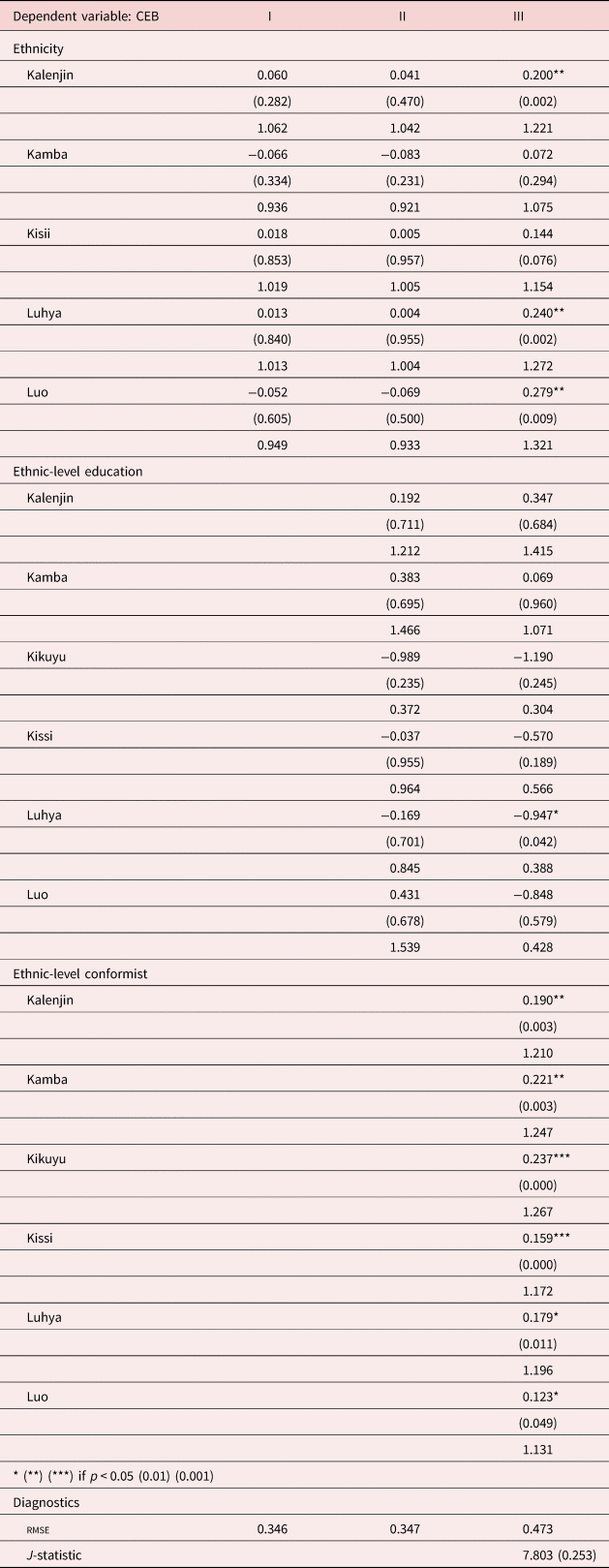
All specifications include the following individual, household, regional, and cluster controls.
Individual: age, age22, dummies for primary, secondary, and higher education.
Individual: dummies for listen to radio, know a place to test for aids.
Household: dummies for tv and radio ownership, mortality.
Household: dummies for: flooring (tile, wood); roof (tiled).
Cluster controls: media access, electricity, water and size of cluster.
Timing: age at first marriage, knowledge of contraception.
Table 9. Religion model: religion and interaction effects
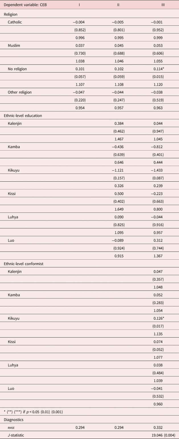
All specifications include the following individual, household, regional, and cluster controls.
Individual: age, age22, dummies for primary, secondary, and higher education.
Individual: dummies for listen to radio, know a place to test for aids.
Household: dummies for tv and radio ownership, mortality.
Household: dummies for: flooring (tile, wood); roof (tiled).
Cluster controls: media access, electricity, water and size of cluster.
Timing: age at first marriage, knowledge of contraception.
Table 10. Ethnicity and religion: ethnicity and interaction effects

All specifications include the following individual, household, regional, and cluster controls.
Individual: age, age22, dummies for primary, secondary, and higher education.
Individual: dummies for listen to radio, know a place to test for aids.
Household: dummies for tv and radio ownership, mortality.
Household: dummies for: flooring (tile, wood); roof (tiled).
Cluster controls: media access, electricity, water and size of cluster.
Timing: age at first marriage, knowledge of contraception.
For each variable, we report three outputs. Parameter estimates, say β j, may be interpreted as the proportional change in the number of CEB due to a unit change in the j th regressor.Footnote 17 Underneath and in parenthesis, we report the p-value, followed by the $e^{{\hat{\beta }}_j}\comma \;$ the factor change [the incidence-rate ratio (IRR)] in the expected count for a unit increase in a given x j. As an example, an IRR = 1.10 indicates a 10% increase in the expected CEB for a one-unit change in x j. We emphasize this statistic when interpreting our results. Standard errors are robust to arbitrary intra-cluster correlation. We also report the J-statistic affording a test of the exogeneity of our instruments. In Table 8, we report the results for our baseline model with ethnic effects. Table 9 reports our results when we include a set of a religion dummies, replacing ethnic effects. Table 10 reports our results, when we include both religious and ethnic effects.
6.1 Ethnicity and religion effects
Table 8 reports our results for the baseline model. Each table presents the results for three specifications. Specification I incorporates traditional fertility determinants at the individual, household, and ethnicity level. Specification II extends I with the addition of ethnic-level exogenous effects (due to education), with specification III adding ethnic-level conformist effects.
Ethnicity effects were significant for all ethnic groups such as the Kalenjin (1.221), the Luhya (1.272), the Kisii (1.154), and for the Luo (1.321), revealing larger fertility effects relative to the Kikuyu which are the reference group. The relative magnitudes of the ethnic effects reflect what the descriptive statistics also show in Table 1 namely that the Kikuyu have the lowest fertility of any of the ethnic groups. Given that in many cases ethnic groups settle in specific regions, it was not possible to separately identify all regional effects.
In Table 9, when we replace ethnicity with religion, the only group for which the effect is significant is for the group with no religion (1.120). In Table 10, when we include both ethnicity and religion, the effects are significant for the ethnic groups Kalenjin (1.216), Luhya (1.270), and Luo (1.323) only, and not significant for any of the religious groups.
6.2 Ethnic-level education effects
We consider exogenous education effects as attributable to the effect of observing the level of education of other women in the same cluster. We measure this effect using the proportion of women who had completed higher education, allowing parameters to differ by ethnicity.Footnote 18
With the exception of the Luhya ethnic group, ethnic-level education effects in Table 8 are insignificant after controlling for individual educational attainment. They are also unimportant in Table 9 when we substitute religion for ethnicity, and they are only significant for the Luhya group (0.386) when we include both ethnicity and religion in Table 10.
6.3 Ethnic-level conformist effects
In Table 8, the localized endogenous effects emanating from within the village cluster are captured by a parameter which, for each ethnic group, reflects the impact of the difference between a cluster mean-level fertility and individual CEB—namely the difference between a mean-level and individual CEB for women who live in the same cluster. We observe that for all six groups, these parameters are significant and positive with effects being strongest for the Kikuyu, ranging from 1.267 for the Kikuyu, 1.247 for the Kamba, 1.209 for the Kalenjin, 1.196 for the Luhya, 1.172 for the Kisii, to 1.131 for the Luo.
We emphasize that these results are consistent with our anthropological understanding of the ethnic groups (as discussed in section 2). Namely, for those clusters in which individuals were related both by blood and marriage, as for example, among the Kikuyu mbari, the endogenous effects on fertility are the strongest of the ethnic group effects. This is important for demographic analyses per se since our results indicate the importance of including a measure which captures the effects of interactions within ethnic groups, and that they are important over and above the individual and household characteristics. This is consistent with anthropological and other studies of fertility outlined in section 2 which also emphasize the role of these social norms. It is also striking that the Kikuyu who demonstrate the lowest average fertility are also those for whom the endogenous effects are the strongest.
In Table 9, we report a model which is identical except we allow for religious effects but exclude ethnicity effects. Using the Christian religion as a reference category, we find that none of the religious effects are significant. The only group for which conformist effects matter are the Kikuyu (1.135). We note that this model fails Hansen's test of overidentifying restrictions.
In Table 10, we report results for a model specification where we allow for religious effects in addition to the role of ethnicity. We again find that religion does not exert any significant incremental effect on the number of CEB. Comparing the results in Tables 8 and 10, we find that the results do not change to any significant degree. For example, in Table 9 with religion, the endogenous effects are all insignificant except for the Kikuyu, while in Table 10 with religion controlled for and ethnicity effects, the endogenous effects for ethnicity are all highly significant. This suggests that the ethnicity social interaction effects which we postulate as being important in this society are upheld even after controlling for the effect of religion.
In Kenya, there is a fair amount of heterogeneity by religion. However, the question is how this potential effect of religion plays out alongside the generalized norms at the level of the ethnic group, which are much stronger in this society. We speculate that one reason why there may not be an effect of religion is that the tribal groups and tribal norms pre-date the introduction of Christianity and Islam in this society, and may also be associated with historical tribal religions, so this might be one reason why the ethnic effects predominate the religion effects. Hence, we maintain the emphasis on ethnicity and the different channels of effects, even after controlling for religion.
6.4 Individual-level effects
We do not report the details of the individual- and household-level effects in Tables 8–10 but discuss them here. As expected, many of the individual-level variables were highly significant: these included the woman's age with an older woman exhibiting higher fertility compared to her younger counterpart. For women, primary and secondary education was significant and positive. Higher education was significant in specification I and as expected, strongly negative.Footnote 19 Primary and secondary education has the expected positive relationship with CEB. Also in specifications I and II, if the woman knows a place to test for AIDS, she was likely to have much lower fertility than if she did not. This effect however disappears when the endogenous effects are included. We control for the effect of an individual's religion, but do not see any effects for this, except for those with no religion in Table 9. These effects disappear entirely when the ethnicity effects are included in Table 10.
6.5 Timing effects
In order to examine the fertility behavior of a group of women whose fertility is largely complete, we restrict the sample to women aged 30–49. We also control for age at first marriage, and knowledge of any method of contraception. Age at marriage exerts a strongly negative effect on fertility. Knowledge of contraception was not significant.
6.6 Household-level effects
Household-level controls are included so as to reduce the possibility that any inference on household-level interaction effects is not confounded by household-level omitted variables. At the household level, we make a distinction between interactions within the household which may have implications for fertility, and household-level controls. None of the household-level interaction effects were significant, except the infant mortality variable at the household level in specifications I and II. The significance of the infant mortality variable which measured whether a son or a daughter had died is consistent with the argument that higher infant mortality usually results in higher fertility as well. Interestingly, when the endogenous effects are included, the significance of this variable disappeared. This might suggest that there are ethnic variations in infant mortality rates, as discussed further below.
In general, we would expect that income would be negatively correlated with fertility. As noted above, one of the problems with the DHS survey is that no direct questions on income were asked of survey respondents. To address this deficiency, a number of household-level variables were included as controls for income and other characteristics. One measure of roofing quality was included to suggest that if the woman lived in a household that was wealthier, as measured by a better quality roof such as a tiled roof, then her CEB was more likely to be lower, relatively to the base category—a thatched roof. If a woman lived in a house which had a tiled floor, the expected number of CEB was likely to be lower than if she was resident in a house with a sand floor. The tiled floor variable emerged as very significant. For the roofing quality variables, if the woman lived in a house which had a tiled roof (relative to the base of thatch), then this might have been important but this was not as significant as floor quality. Two variables included in the models which could be construed both as income indicators and as controls for media access are radio and television ownership. Television ownership was strongly negatively significant in specifications I and II, but not radio ownership, in the models with no endogenous effects.
7. Conclusion
Strategic complementarities in fertility decisions imply that a couple's fertility decisions may be dependent on the actions of others in the vicinity or in the society more widely. The mechanisms through which these complementarities occur are through social interactions. This paper has examined social interactions in the context of fertility behavior in Kenya. We have examined the role of dependencies across individuals that reside in a cluster of households and who locate according to ethnicity. More significantly, we emphasize the existence of multiple channels of social interaction. Our results confirm strongly the importance of ethnic-level effects alongside the traditional determinants of fertility at the individual level such as religion. After controlling for the timing effects, endogenous effects, household, and individual effects, the exogenous effects are insignificant. This might suggest that social interactions matter more at the level of the extended group—in this instance, localized interactions through village clusters and more global interactions through ethnic effects. We do not find any significant effects of religion. In the context of a wider debate about multiple identities, this seems to suggest that the effects of ethnicity may outweigh the effects of religion in this society.
Given their significance as our results show, we feel that more research needs to be done on these effects and the broader relationship between demography and cultural networks such as ethnicity and religion. Our results suggest that in considering a continuum of interactions from the most local, i.e., the individual to the most global, the ethnic group, kin groups, and the structure of the network of women's interactions may be more important to fertility decision-making than interactions that take place at the level of the household. This could well be a function of how attitudes and norms related to high fertility might be changing. For example, as women are better informed about matters related to fertility decision-making beyond their immediate household, whether through the media or through other channels, this knowledge influences norms and exerts a greater influence on their decision-making. Our research is of course unable to solve this puzzle precisely because data on networks were not collected in the KDHS survey, but it does suggest that more research is required to identify the precise form of the interactions operating among kin groups, religious, and ethnic groups, and how they affect fertility preferences in Kenya and elsewhere, where ethnicity, religion, and fertility outcomes are linked.
Acknowledgements
For helpful comments and discussions, we are grateful to the Editor Jared Rubin, Wiji Arulampalam, Ethan Cohen-Cole, Partha Dasgupta, Gernot Doppelhofer, Steven Durlauf, Timothy Guinnane, Andrew Harvey, Larry Iannaccone, Hashem Pesaran, Richard Smith, and Chander Velu. We acknowledge funding from the Centre for Research in Microeconomics, and St. Catharine's College, Cambridge. We are grateful to Zipporah Onchari and the Director of the Kenya Meteorological Services for giving us access to their rainfall data. We thank Anne Mason, Chris Brown, and Tirthankar Chakravarty for excellent research assistance. We are also grateful for many helpful suggestions provided by seminar participants at George Mason University, University of Wisconsin-Madison, University of Warwick, the School of Oriental and African Studies, University of London, University of Cambridge, and the Brookings Institution.
Appendix A
The Generalized Method of Moments (GMM) estimator
In this paper we adopt the Generalized Method of Moments (GMM) estimator. A GMM estimator is particularly suited to this particular context, since by using first-order conditions only, it allows for unobserved heterogeneity without a full set of parametric assumptions (i.e., the Poisson variance assumption), and accommodates endogenous regressors. Whereas the fully parametric mixture extensions of the Poisson regression model, such as the negative binomial and zero-inflated Poisson models, impose statistical independence between the unobserved heterogeneity and ${\bi x}_i$ , a GMM framework readily accommodates dependence.
The GMM estimator minimizes the (generalized) length of the empirical vector function

where ${\bi w}$ collects all observables including instrumental variables ${\bi z}$
 . The nature of the conditional moment restrictions, ${\bi \psi }_N\lpar. \rpar$
 will depend upon whether we introduce an additive or multiplicative error structure. As noted by Windmeijer and Santos-Silva (Reference Windmeijer and Santos-Silva1996), although multiplicative and additive models are observationally equivalent when only the first-order conditional mean is specified, there are differences in the presence of endogeneity and the subsequent choice of instruments in the two specifications. Given $E\lpar {c_i\vert {\bi x}_i} \rpar = \exp \lpar {{\bi x}_i^{\prime} {\bi \beta }} \rpar$
 , the additive model implies $c_i = \exp \lpar {{\bi x}_i^{\prime} {\bi \beta }} \rpar + \omega _i$
 , with moment conditions $E\lpar {\bi z}_i^{\prime} \lpar {c_i-\exp \lpar {{\bi x}_i^{\prime} {\bi \beta }} \rpar } \rpar$
 . The multiplicative modelFootnote 20 posits $c_i = \exp \lpar {{\bi x}_i^{\prime} {\bi \beta }} \rpar \omega _i$
 , with moment conditions $E\lpar {{\bi z}_i^{\prime} \lpar {c_i\cdot \exp \lpar {-{\bi x}_i^{\prime} {\bi \beta }} \rpar -1} \rpar } \rpar$
 . The multiplicative model handles regressors ${\bi x}_i$
 and error terms ω i in a symmetric fashion. In addition, given that for c not equal to zero, ${\rm ln\;}c_i = {\bi x}_i^{\prime} {\bi \beta } + \omega _i$
 is congruent with the GLM.
Given a multiplicative error model ${\bi \psi }_N\lpar {\bi w}\comma \;{\bi \beta }\rpar = {\bi {Z}^{\prime}}\lpar {c-\kappa \lpar {\bi \beta } \rpar {\rm \bond /}\kappa \lpar {\bi \beta } \rpar } \rpar \comma \;\kappa \lpar {\bi \beta } \rpar = \exp \lpar {{\bi {X}^{\prime}\beta }} \rpar$ . We can write (A.1) as

where ${\bi Z} = \lcub {{\bi z}_i} \rcub$ denotes an instrument matrix.Footnote 21 $\tilde{Q}_N = {\bi {Z}^{\prime}\Omega Z}$
 denotes the optimal weight matrix where ${\bi \Omega } = \lpar {c-\kappa \lpar {\hat{{\bi \beta }}} \rpar {\rm /}\kappa \lpar {\hat{{\bi \beta }}} \rpar } \rpar ^2$
 . $\kappa \lpar {\hat{\bi \beta}} \rpar = \exp \lpar {{\bi {X}^{\prime}}\hat{\bi\beta }} \rpar$
 with $\hat{{\bi \beta }}$
 a first step GMM estimator based upon any weighting matrix.
Appendix B
Conformist effects
In the conditional mean specification (3), conformist effects are represented by cfi,g = E i(c g) − c i, where c i denotes the number of children (CEB) ever born to the i th woman, and E i(c g) is the expectation of mean CEB held by the i th woman resident in cluster g. This formulation contains two components: E i(c g) represents the expectation of average fertility of the i th woman in group g. Assuming that each woman possesses rational expectations on E i(c g), then individual expectations of average fertility behavior in the group equals the average behavior such that $E_i\lpar {c_g} \rpar = N_g^{{-}1} \mathop \sum \nolimits_{i\in g}c_i$ , where N g denotes the number of individuals in the group. We argue that the rational expectations are valid given that cluster sizes are small. For example, in Blume et al. (Reference Blume, Brock, Durlauf, Ioannides, Benhabib, Jackson and Bisin2010), it is argued that identification of social interaction effects may depend on whether individuals are reacting to the expected or actual behavior of others. If the sample sizes are small, then assumptions such as complete information and the individual's payoff depending on the actual choices of others in the group, rather than on expectations about the average choice of others, is justified by the study of interactions in relatively small groups. For example, individuals may have incentives to conform to the behavior of a small number of appropriately defined neighbors whose actions they can “observe”.
Below we represent these arguments more formally. Suppose U i denotes the utility function of household i, c i represents the number of children, ${\bi l}_i$ is all sources of satisfaction to the husband and wife other than those arising from children, and ${\bi x}_i$
 denotes the vector of socio-demographic characteristics which affect preferences. We extend the standard atomistic utility model of fertility to incorporate a theory of social interactions, so we can write

where V i, total individual utility, is comprised of a private utility term $U\lpar {c_i\comma \;{\bi l}_i\comma \;{\bi x}_i} \rpar \comma \;$ and a social utility term: $S^j\lpar {c_i\comma \;{\bi c}_{{-}i}^j } \rpar$
 which represents utility for location or ethnicity j, given by some function of the number of children choices made by all other residents of j; ${\bi c}_{{-}i}^j = \lpar {c_{1\comma }^j c_2^j \comma \;\ldots \comma \;c_{i-1}^j \comma \;c_{i + 1}^j \comma \;\ldots \comma \;n_{M_j}^j } \rpar$
 , where M j denotes the number of individuals in location j. The extension allows us to capture that component of individual utility attributable to a fertility choice c i that is dependent upon the fertility choices of others. The “others” in question may be those, for example, resident in the individual's household, or others resident in the local community for example, in the individual's street or neighborhood, religion, or members of the same ethnic group or tribe. Rewriting (B.1) as additive in individual and social utility terms, and without loss of generality, we have

The addition of the social utility function S j(.) represents a model in which we allow individual behavior to be partially determined by the collective decisions of a group. Differentiating the Beckerian first-order conditions with respect to social interactions yields the second-order conditions

where $\kappa _{il}^j$ represents a measure of the disutility accruing to i from deviating from the behavior of l for i, l ∈ j.
The form of social utility at the level of location j may be written as

where (7) represents social utility as a measure of conformism with $\partial S_{}\lpar. \rpar /\partial c_i = \theta _2\lpar {\bar{c}_{{-}i}^j -c_i} \rpar.$ Under (B.3) there is an incentive to conform to mean fertility behavior within the group with deviations from the mean penalized. If behaving like others confers additional status on a woman, she may desire to conform.Footnote 22
Appendix C
The identification problem
The nature of the identification problem in models of social interaction is complex. Below we consider a number of dimensions to this problem, namely: the presence of timing effects, Manski's reflection problem, the endogeneity of mean effects, and identification of interaction effects. Such timing effects, for example, younger cohorts marrying at later ages, are important in that they determine, in part, the distance between the observed number of children for any given woman and the mean number of children in the appropriate reference group. This difference is central to our thesis, namely that changes in this distance will impact upon CEB due to an interaction effect. Below we address each of these issues, and in doing so outline our identification strategy.
In considering the relevance of the reflection problem for our particular application, we first outline the identification problem in the linear-in-means social interaction model as originally considered by Manski (Reference Manski1993), and more recently by Blume et al. (Reference Blume, Brock, Durlauf, Ioannides, Benhabib, Jackson and Bisin2010) and Ioannides (Reference Ioannides, Blume and Durlauf2008). Since the question of identification is well understood in the linear framework, this will provide a useful point of departure. Using what is now common notation for this problem, a linear model of fertility behavior may be written as

where ${\bi q}_i$ denotes a K × 1 vector of individual characteristics, ${\bi y}_g$
 is a L × 1 vector of exogenous (contextual) characteristics and $m_{ig}^e$
 denotes the expected average fertility of others in the group held by the i th woman. ${\bi \eta }$
 , ${\bi \lambda }$
 , and κ denote unknown parameters. Under a rational expectations assumption, we may write $m_{ig}^e = m_g = \alpha + \bar{{\bi q}}^{\prime}{\bi \eta } + {\bi y}_g^{\prime} {\bi \lambda }$
 . If we then impose the restriction that the dimension of $\bar{{\bi q}}$
 is the same as ${\bi y}_g$
 , then m g may be written as

In this context, Manski's reflection problem is immediately seen. Namely, any observed correlation between an outcome c i and m g solely reflects the combined effect of mean-group characteristics, ${\bi y}_g$ , rather than endogenous interaction within a group. The genesis of the reflection problem derives from the fact that in (C.1) we specify a model for CEB which is linear in an endogenous effect, $m_{ig}^e$
 , a vector of exogenous effects, ${\bi y}_g$
 , and a vector of individual characteristics, ${\bi q}_i$
 . If the number of exogenous and individual effects is equivalent, it then follows that the reduced form representation of the conditional mean will be a function of ${\bi y}_g$
 .Footnote 23
There are a number of ways to circumvent the reflection problem. Within a linear framework, the simplest method is to impose a full set of zero restrictions on ${\bi \lambda }$ , thereby adopting the assumption that any interactions are mediated solely by endogenous effects. We note that such an approach is potentially problematic for making inference on multiplier effects, since such restrictions may result in biased estimates of pure endogenous effects [see Ioannides (Reference Ioannides, Blume and Durlauf2008)]. This is important since policy prescriptions which follow from endogenous versus exogenous effects are likely to be very different. However, the upside of such an approach is that these restrictions automatically generate a possible set of instruments $\lpar {\bi q} \rpar$
 for m g.Footnote 24 Second, and as discussed earlier, identification is facilitated by locating one or more individual-level variables whose group-level average does not enter the conditional mean.
In this study, the reflection problem is mitigated for a number of reasons. First, although it is possible to conceive of a large number of exogenous effects, in the specific context of fertility behavior, education plays a particularly prominent role. Numerous studies in developed and developing countries have argued that education is the single most important predictor of fertility decline. This is because education increases the opportunity cost of women's time, and encourages parents to have higher quality children, which then reduces women's fertility. Moreover, better educated women are likely to exert an influence on less educated women if they provide effective role models for them. It is for this reason that we focus primarily on this exogenous effect. Second, given that the conditional mean specification represents a non-linear transformation of the endogenous effect, then even if the restriction $\bar{{\bi q}} = {\bi y}_g$ held, identification would be achieved.
Endogeneity bias
Given the form of endogenous conformist effects, namely cfi,g = E i(c g − c i), we face a variant of the mean endogenous effects problem. In tackling this problem, we adopt an instrumental variable approach. However, the required condition that an instrument may only impact c i indirectly through its association with cfi,g may not hold given that cfi,g is a linear function which includes c i.
We address this problem by an appropriate specification of the conditional mean. Given that the mean of a count process has non-negative support, we specify conditional mean of CEB as an exponential function of a linear index in the regressors. As a consequence, the otherwise linear dependence between the original error term, ω i, and the instrument is removed given the imposition of a restriction on the support of the conditional mean using the exponential functionFootnote 25. It is important to emphasize that the nature of our identification strategy is not dependent on a highly specific set of parametric assumptions but rather a minimal set of assumptions to ensure the non-negativity of the conditional mean. Blume et al. (Reference Blume, Brock, Durlauf, Ioannides, Benhabib, Jackson and Bisin2010) make a similar argument in outlining conditions for identification in other non-linear social interaction models.Footnote 26
Given that the number of instruments excluded exceeds the number of endogenous variables, our estimating equation is overidentified, and we may evaluate the validity of our instruments by testing whether the excluded instruments are independent of the error process using the J-test [see Hansen (Reference Hansen1982)]. This statistic is the value of CEB objective function, evaluated at the efficient CEB estimator. Under the joint null hypothesis of correct model specification and the validity of the orthogonal conditions, the J-statistic is given by

where $\hat{{\bi u}}$ denotes the residuals and l–k denotes the number of overidentifying restrictions. $\hat{\Omega }_C$
 represents a form of the error covariance matrix which is robust to arbitrary intra-cluster correlation.Footnote 27 A rejection of the null may then result from the instruments not satisfying the orthogonality conditions given they are not exogenous or because they are incorrectly excluded.


 Open access