2.1. Governing equations

As in Yim et al. (Reference Yim, Billant and Gallaire2020), we consider an axisymmetric vortex with initial non-dimensional velocity $\boldsymbol {u}_0=(u_0,v_0,w_0)= (0, r \exp (-r^2),0)$ in cylindrical coordinates $(r,\theta, z)$. The time and length have been chosen so that the vortex radius and the maximum angular velocity are unity. The fluid is incompressible and rotating about the $z$ axis:

(2.1)\begin{gather} \displaystyle{\frac{\partial {\boldsymbol{u}}}{\partial {t}}}+ \boldsymbol{u} \boldsymbol{\cdot} \boldsymbol{\nabla} \boldsymbol{u}+ 2\,Ro^{{-}1} \boldsymbol{e}_z \times \boldsymbol{u}={-} \rho^{{-}1}\,\boldsymbol{\nabla} p + Re^{{-}1}\,\nabla^2 \boldsymbol{u}, \end{gather}

(2.2)\begin{gather}\boldsymbol{\nabla} \boldsymbol{\cdot} \boldsymbol{u} =0, \end{gather}

where $\boldsymbol {e}_z$ is the unit vector in the $z$ direction, $p$ is the pressure, $\rho$ is the constant density, $Ro=2\varOmega _c/f$ is the Rossby number, and $Re=\varOmega _cR_0^2/\nu$ is the Reynolds number, with $f$ the Coriolis parameter, $\varOmega _c$ and $R_0$ the dimensional maximum angular velocity and radius of the vortex, and $\nu$ the viscosity.

Yim et al. (Reference Yim, Billant and Gallaire2020) studied the particular value $Ro=-4$ for several Reynolds numbers and showed that the dynamics remains always purely axisymmetric. For this reason, axisymmetry will be assumed here from the outset. The boundary conditions are therefore $u = v = 0$ at $r=0$, and $\boldsymbol {u} \to 0$ as $r \to \infty$ (Batchelor & Gill Reference Batchelor and Gill1962). The Rossby number will be also set to $Ro=-4$ throughout the paper, as in Yim et al. (Reference Yim, Billant and Gallaire2020).

2.2. Mean and fluctuation equations

Following Stuart (Reference Stuart1958), Davey (Reference Davey1962) and Yim et al. (Reference Yim, Billant and Gallaire2020), it is first convenient to decompose the velocity and pressure as

(2.3)\begin{equation} [\boldsymbol{u},p](r,z,t) = [\bar{\boldsymbol{U}},\bar{P}](r,t) + [\hat{\boldsymbol{u}},\hat p](r,z,t), \end{equation}

where $\bar {\boldsymbol {U}}=z_{max}^{-1} \int _0^{z_{max}} \boldsymbol {u}\,\mathrm {d} z$ and $\bar {P}=z_{max}^{-1} \int _0^{z_{max}}p\,\mathrm {d} z$ are the axially averaged mean quantities over the domain height $z_{max}$. Averaging (2.1)–(2.2) in $z$ shows that the mean flow is purely azimuthal, $\bar {\boldsymbol {U}}=\bar {V}(r,t)\,\boldsymbol {e}_{\theta }$, and governed by

(2.4)\begin{gather} -\frac{\bar{V}^2}{r}-\displaystyle{\frac{2}{Ro}}\,\bar{V} ={-}\rho ^{{-}1}\,\displaystyle{\frac{\partial {\bar{P}}}{\partial {r}}} - \overline{\mathcal{N}(\hat{\boldsymbol{u}},\hat{\boldsymbol{u}})} \boldsymbol{\cdot} \boldsymbol{e}_r, \end{gather}

(2.5)\begin{gather}\frac{\partial \bar{V}}{\partial t} = \frac{1}{Re}\,D^2\bar{V} - \overline{\mathcal{N}(\hat{\boldsymbol{u}},\hat{\boldsymbol{u}})} \boldsymbol{\cdot} \boldsymbol{e}_\theta, \end{gather}

where

(2.6)\begin{gather} D^2 \cdot{} = \frac{\partial}{\partial r}\left(\frac{1}{r}\,\frac{\partial}{\partial r}\left(r {\cdot} \right) \right), \end{gather}

(2.7)\begin{gather}\mathcal{N}(\boldsymbol{a},\boldsymbol{b}) =\boldsymbol{a} \boldsymbol{\cdot} \boldsymbol{\nabla} \boldsymbol{b} {=\begin{pmatrix} a_r\,\displaystyle{\frac{\partial b_r}{\partial r}}+a_z\,\displaystyle{\frac{\partial b_r}{\partial z}}-\displaystyle{\frac{a_\theta b_\theta}{r}}\\[6pt] a_r\,\displaystyle{\frac{\partial b_\theta}{\partial r}}+a_z\,\displaystyle{\frac{\partial b_\theta}{\partial z}}+\displaystyle{\frac{a_\theta b_r}{r}}\\[6pt] a_r\displaystyle{\frac{\partial b_z}{\partial r}}+a_z\,\displaystyle{\frac{\partial b_z}{\partial z}} \end{pmatrix}}. \end{gather}

It is convenient to further decompose the mean flow as

(2.8)\begin{equation} \bar{V}(r,t)=v_0(r)+ \bar{v}(r,t), \end{equation}

where $v_0$ is the initial flow, so that (2.5) becomes

(2.9)\begin{equation} \frac{\partial \bar{v}}{\partial t} = \frac{1}{Re}\,D^2(\bar{v} +v_0)- \overline{\mathcal{N}(\hat{\boldsymbol{u}},\hat{\boldsymbol{u}})} \boldsymbol{\cdot} \boldsymbol{e}_\theta. \end{equation}

Subtracting (2.4) and (2.9) from (2.1) yields the equation for the perturbation $\hat {\boldsymbol {u}}$:

(2.10) \begin{gather} \frac{\partial \hat{\boldsymbol{u}}}{\partial t}+ \mathcal{L}(\hat{\boldsymbol{u}}) ={-}\mathcal{N}(\boldsymbol{\bar{u}},\hat{\boldsymbol{u}})- \mathcal{N}(\hat{\boldsymbol{u}},\boldsymbol{\bar{u}})-\mathcal{N}(\hat{\boldsymbol{u}},\hat{\boldsymbol{u}}) +\overline{\mathcal{N}(\hat{\boldsymbol{u}},\hat{\boldsymbol{u}})}, \end{gather}

(2.11)\begin{gather}\boldsymbol{\nabla}\boldsymbol{\cdot} \hat{\boldsymbol{u}} =0, \end{gather}

where $\boldsymbol { \bar {u}}=\bar {v}\boldsymbol {e}_\theta$ and

(2.12)\begin{equation} \mathcal{L}(\hat{\boldsymbol{u}}) ={-}2 \varOmega_0\hat v\boldsymbol{e}_r + \zeta_0\hat u\boldsymbol{e}_\theta + 2\,Ro^{{-}1}\boldsymbol{e}_z \times \hat{\boldsymbol{u}} + \rho^{{-}1}\,\boldsymbol{\nabla} \hat{p} -Re^{{-}1}\,\nabla^2 \hat{\boldsymbol{u}},\end{equation}

with $\varOmega _0=v_0/r$ and $\zeta _0=2\varOmega _0+r\varOmega _0'$. We emphasize that (2.9)–(2.11) are only a convenient rewriting of (2.1)–(2.2), and no approximation has been done so far. In the absence of perturbation $\hat{\boldsymbol {u}}=0$, the total mean flow $\bar {V}$ is governed by the diffusion equation (2.5) and there is a cyclostrophic balance along the radial direction (2.4).

2.3. Linear stability

When (2.10)–(2.11) are linearized and the viscous diffusion of the base flow is neglected so that $\bar {v}=0$, they reduce to the stability problem

(2.13)\begin{gather} \frac{\partial \hat{\boldsymbol{u}}}{\partial t}={-} \mathcal{L}(\hat{\boldsymbol{u}}), \end{gather}

(2.14)\begin{gather}\boldsymbol{\nabla} \boldsymbol{\cdot} \hat{\boldsymbol{u}} =0. \end{gather}

Here, we will consider the weakly nonlinear evolution of the most unstable perturbation of (2.13) for a given axial wavenumber $k$:

(2.15)\begin{equation} [\hat{\boldsymbol{u}},\hat p]= [\tilde{\boldsymbol{u}},\tilde{p}](r)\exp (\sigma t +{\rm i}k z) +c.c., \end{equation}

where $\sigma$ is the growth rate and $c.c.$ denotes the complex conjugate.

When the Rossby number is in the range $Ro < -1$ or $Ro > \exp (2)$, a vortex with Gaussian angular velocity is unstable in the inviscid limit to the centrifugal instability according to the Rayleigh criterion, i.e. there exists some radius where $\phi < 0$, with $\phi =2(\varOmega _0 + 1/Ro)(\zeta _0+2/Ro )$ the Rayleigh discriminant. The inviscid growth rate is given by $\sigma _i=\sqrt {-\phi (r_0)}$, where $r_0$ is the radius where $\phi$ is minimum (Smyth & McWilliams Reference Smyth and McWilliams1998; Billant & Gallaire Reference Billant and Gallaire2005) ($r_0=0.93$ and $\sigma _i=0.3635$ for $Ro=-4$) and is reached in the limit of infinite axial wavenumber. When the Reynolds number is finite, the maximum growth rate and the most amplified wavenumber $k_m$ decrease as the Reynolds number is reduced, as illustrated in figure 1(a) for $Ro=-4$. The instability is totally stabilized when $Re \sim 100$. Since viscous effects scale like $k^2/Re$ at leading order for large axial wavenumber, they become active for wavenumbers typically such that $k^2=O(Re)$.

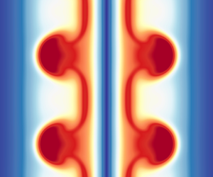
Figure 1. (a) Linear growth rate $\sigma$ as a function of the axial wavenumber $k$ for $Ro=-4$ and different Reynolds numbers: $Re=150$, $500$, $1000$, $2000$ and $3000$. The red circles indicate the maximum growth rate and corresponding most amplified axial wavenumber $k$. (b) Velocity components $(\tilde u,\tilde v,\tilde w)$ of the eigenmodes as functions of $r$ for $k=8.6$ (blue lines) and $k=23$ (black lines), for $Re=2000$ and $Ro=-4$. (c) Same as (b), but the velocity components are rescaled as $(\tilde u/\sqrt {k},\tilde v/\sqrt {k},\tilde w)$ and plotted as functions of $\tilde r=(r-r_0)\sqrt {k}$.

Figure 1(b) displays the eigenmodes for $Re=2000$ for two wavenumbers: $k=8.6$ and $k=23$. As in Yim et al. (Reference Yim, Billant and Gallaire2020), the eigenmode is normalized so that the maximum absolute vertical velocity is unity: $\max ( | \tilde w | )=1$. It can be seen that the eigenmode tends to be more localized as $k$ increases and the amplitudes of the horizontal velocity components increase with $k$.

3.1. Formulation

The first task in order to carry out a weakly nonlinear analysis is to identify some conditions under which the instability is only marginally unstable. There are several possible configurations: first, the Rossby number can be considered close to the critical Rossby numbers $Ro_c=-1$ or $Ro_c'=\exp (2)$; second, $Ro$ can be considered arbitrary but $Re$ close to the critical Reynolds number $Re_c$ (figure 1); or, third, $Ro$ and $Re$ can be considered arbitrary but the axial wavenumber $k$ can be assumed to be close to the viscous cut-off $k_c$ where the growth rate vanishes (figure 1). Since the Rossby number $Ro=-4$ investigated in Yim et al. (Reference Yim, Billant and Gallaire2020) is relatively far from $Ro_c=-1$, we will consider herein the second configuration, i.e. the Reynolds number $Re$ is assumed to be close to $Re_c$ so that the eigenmode at the most unstable wavenumber $k$ for this Reynolds number $Re$ is marginally unstable. However, we will see later that the following analysis will also apply to the third configuration, i.e. near the viscous wavenumber cut-off. Accordingly, the order of magnitude of the growth rate can be used as a small parameter, i.e.

(3.1)\begin{equation} \sigma= \epsilon\tilde{\sigma}, \end{equation}

where $\tilde {\sigma }=O(1)$ and $\epsilon \ll 1$. Even if the Reynolds number is close to $Re_c$, we will consider that it is large such that

(3.2)\begin{equation} \frac{1}{Re}=\frac{\epsilon^2}{\widetilde{Re}}, \end{equation}

with $\widetilde {Re}=O(1)$. This distinguished limit will enable us to take into account the viscous diffusion at leading order. Nevertheless, the following analysis should remain valid if $1/Re \lesssim O(\epsilon ^2)$, i.e if the Reynolds number is larger than imposed by (3.2), but not in the opposite case, $1/Re \gg O(\epsilon ^2)$. Hence the scaling assumptions (3.1) and (3.2) can be combined into the condition $1/\sqrt {Re} \lesssim \sigma \ll 1$, meaning that the growth of the perturbation has to be slow but not too slow compared to the viscous diffusion. A paradoxical implication is that as the Reynolds number decreases (figure 1a), our approach will no longer be valid below a certain Reynolds number even if the growth rate is small, because the condition $1/\sqrt {Re} \lesssim \sigma$ will no longer be fulfilled. For the same reason, if the Rossby number is increased from below towards the critical value $Ro_c=-1$ for a fixed large Reynolds number, the present analysis will cease to be valid when $\sigma$ is typically smaller than $1/\sqrt {Re}$. In summary, we expect the scaling hypotheses (3.1) and (3.2) to be met only in an intermediate range of growth rate for given Reynolds and Rossby numbers. This will be confirmed in § 6 when the predictions of the weakly nonlinear analysis will be compared to DNS.

The scaling (3.2) together with the assumption of being close to the viscous threshold, i.e. $\sigma \simeq \sigma _i-k^2/Re \ll 1$, implies that $k^2/Re=O(1)$ since the maximum growth rate in the inviscid limit $\sigma _i$ is of order unity for $Ro=-4$. In this way, viscous effects act on the perturbation despite the large Reynolds number limit considered in (3.2).This implies that the wavenumber is large:

(3.3)\begin{equation} k=\frac{\tilde k}{\epsilon}, \end{equation}

where $\tilde k=O(1)$. An unstable eigenmode is always accompanied by a stable counterpart with opposite growth rate in the inviscid limit due to time reversibility. Hence if the unstable eigenmode is marginally unstable, then the stable counterpart is also marginally stable and it needs to be taken into account in a weakly nonlinear analysis. However, (3.2) and (3.3) imply that such a stable mode is here strongly damped and does not need to be considered since its growth rate is $\sigma \simeq -\sigma _i-k^2/Re$, which is typically $O(1)$ and negative. For that reason, the resulting amplitude equations will be first order in time and dissipative, while similar inviscid instabilities in nature, such as the baroclinic instability or the Kelvin–Helmholtz instability, have been described by amplitude equations that are second order in time and thus reversible (Drazin Reference Drazin1970; Pedlosky Reference Pedlosky1970; Gibbon & McGuinness Reference Gibbon and McGuinness1981).

In turn, the fact that the wavenumber is large implies that the eigenmode $[\tilde{\boldsymbol {u}},\tilde p](r)$ is strongly localized in a region of width $O(k^{-1/2})=O(\epsilon ^{1/2})$ around a particular radius $r_0$, as shown by Bayly (Reference Bayly1988). Hence the radial derivative is large,

(3.4)\begin{equation} \displaystyle{\frac{\partial {}}{\partial {r}}} = O(k^{1/2}), \end{equation}

meaning that each term of (2.10) needs first to be appropriately scaled before performing a weakly nonlinear analysis. We emphasize that the scaling (3.4) applies only to the perturbation $\hat {\boldsymbol {u}}$ and not to the initial mean flow ${v_0}$. Since the eigenmode is normalized such that $\max (|\tilde w |)=1$, the different velocity components and pressure of the disturbance then scale as (Bayly Reference Bayly1988)

(3.5a–d)\begin{equation} \hat u=O(k^{1/2}),\quad \hat v=O(k^{1/2}),\quad \hat w=O\left(1\right),\quad \hat p=O(k^{{-}1}). \end{equation}

Again, we stress that this scaling does not apply to the mean flow $\bar {v}$. In order to illustrate this scaling, the eigenmodes for $k=8.6$ and $k=23$ are rescaled according to (3.5a–d) and plotted as functions of $(r-r_0)\sqrt {k}$ in figure 1(c). The velocity components for the two wavenumbers collapse, although this is only approximate since $k$ is not so large.

We will use the scaling (3.5a–d) only to obtain the leading-order magnitude of each operator in (2.10) since the linear problem will be solved numerically and not analytically as done by Bayly (Reference Bayly1988). Using (3.4) and (3.5a–d), we have

(3.6a–d)\begin{equation} \mathcal{L}=O(1),\quad \mathcal{N} = O(k), \quad D^2=O(k), \quad \boldsymbol{\nabla}=O(k). \end{equation}

Hence we define the following rescaled variable and operators:

(3.7a–d)\begin{equation} \tilde r= \frac{r-r_0}{\epsilon^{1/2}},\quad \tilde{\mathcal{N}} = \epsilon \mathcal{N}, \quad \tilde D^2=\epsilon D^2, \quad \tilde{\boldsymbol{\nabla}}=\epsilon \boldsymbol{\nabla}, \end{equation}

where the operators with a tilde are of order unity at leading order. These operators could be split into different orders, e.g. $\tilde{\mathcal{N}}=\tilde{\mathcal{N}}_0+\epsilon ^{1/2}\tilde{\mathcal{N}}_1+\cdots$. However, this will not be done, to avoid long algebra. In addition, this is not necessary because the problem will be solved numerically as mentioned already.

Then the governing equations for the perturbation become

(3.8)\begin{gather} \displaystyle{\frac{\partial {\hat{\boldsymbol{u}}}}{\partial {t}}} ={-}\mathcal{L}(\hat{\boldsymbol{u}}) -\epsilon^{{-}1}\,\tilde{\mathcal{N}}( \boldsymbol{ \bar{u}},\hat{\boldsymbol{u}})-\epsilon^{{-}1}\, \tilde{\mathcal{N}}(\hat{\boldsymbol{u}},\boldsymbol{ \bar{u}})- \epsilon^{{-}1}\,\tilde{\mathcal{N}}(\hat{\boldsymbol{u}},\hat{\boldsymbol{u}}) + \epsilon^{{-}1}\, \overline{\tilde{\mathcal{N}}(\hat{\boldsymbol{u}},\hat{\boldsymbol{u}})}, \end{gather}

(3.9)\begin{gather}\tilde{\boldsymbol{\nabla}} \boldsymbol{\cdot} \hat{\boldsymbol{u}} = 0, \end{gather}

The important feature in (3.8) is that the nonlinear terms scale at leading order as $1/\epsilon$ because the axial wavenumber is large. Similarly, the equation for the mean flow (2.9) becomes

(3.10)\begin{equation} \frac{\partial \bar{v}}{\partial t} = \displaystyle{\frac{\epsilon}{\widetilde{Re}}}\,\tilde D^2 \bar{v}+ \displaystyle{\frac{\epsilon^2}{\widetilde{Re}}} D^2 v_0 - \epsilon^{{-}1}\,\overline{\tilde{\mathcal{N}}(\hat{\boldsymbol{u}},\hat{\boldsymbol{u}})} \boldsymbol{\cdot}\boldsymbol{e}_\theta. \end{equation}

We can remark that the viscous diffusion of the mean flows $\bar {v}$ and $v_0$ are not of the same order because the former varies over $\tilde r$ according to (3.4), in contrast to the latter, which varies over $r$.

Nevertheless, (3.8)–(3.10) can be rewritten in a form close to the original (2.9)–(2.11) by simply rescaling the variables as $\overline v = \epsilon \overline v'$ and $[\hat{\boldsymbol {u}},\hat p] = \epsilon [\hat{\boldsymbol {u}}',\hat p']$. This leads to

(3.11)\begin{gather} \displaystyle{\frac{\partial {\hat{\boldsymbol{u}}'}}{\partial {t}}} ={-}\mathcal{L}(\hat{\boldsymbol{u}}') - \tilde{\mathcal{N}}( \boldsymbol{\bar{u}'},\hat{\boldsymbol{u}}')-\tilde{\mathcal{N}}(\hat{\boldsymbol{u}}',\boldsymbol{ \bar{u}'})- \tilde{\mathcal{N}}(\hat{\boldsymbol{u}}',\hat{\boldsymbol{u}}') + \overline{\tilde{\mathcal{N}}(\hat{\boldsymbol{u}}',\hat{\boldsymbol{u}}')}, \end{gather}

(3.12)\begin{gather}\tilde{\boldsymbol{\nabla}} \boldsymbol{\cdot} \hat{\boldsymbol{u}}' = 0, \end{gather}

(3.13)\begin{gather}\frac{\partial \overline{v'}}{\partial t} = \displaystyle{\frac{\epsilon}{\widetilde{Re}}}\,\tilde D^2 \bar{v}'+\displaystyle{\frac{\epsilon}{\widetilde{Re}}}\,D^2 v_0 - \overline{\tilde{\mathcal{N}}(\hat{\boldsymbol{u}}',\hat{\boldsymbol{u}}')}\boldsymbol{\cdot}\boldsymbol{e}_\theta. \end{gather}

The governing equations are now in a suitable form to carry out the weakly nonlinear analysis. To do so, we expand the time, the mean flow and the perturbation as follows:

(3.14)\begin{gather} \displaystyle{\frac{\partial {}}{\partial {t}}} = \displaystyle{\frac{\partial {}}{\partial {t_0}}}+\epsilon\,\displaystyle{\frac{\partial {}}{\partial {t_1}}}+ \epsilon^2\,\displaystyle{\frac{\partial {}}{\partial {t_2}}}+\cdots, \end{gather}

(3.15)\begin{gather}\overline v' = \epsilon \bar{v}_{1}+ \epsilon^2 \bar{v}_{2} +\cdots, \end{gather}

(3.16)\begin{gather}{}[\hat{\boldsymbol{u}}',\hat p'] = \epsilon [\hat{\boldsymbol{u}}_1, \hat p_1]+ \epsilon^{2} [\hat{\boldsymbol{u}}_2, \hat p_2] + \cdots. \end{gather}

In the following, the first-order mean flow will be further decomposed into two parts:

(3.17)\begin{equation} \bar{v}_{1}= \bar{v}_{11}(\tilde r,t_1)+\bar{v}_{10}(r,t_0), \end{equation}

where $\bar {v}_{10}$ will vary over $r$ due to the viscous diffusion of the base flow, whereas $\bar {v}_{11}$ will vary over $\tilde r$ due to its own viscous diffusion and the Reynolds stresses due to the perturbation.

Finally, we stress that we will consider a single axial wavenumber, i.e. no spatial modulation will be taken into account in the present analysis. The DNS performed by Yim et al. (Reference Yim, Billant and Gallaire2020) for $Ro=-4$ and $Re=2000$ initialized by the eigenmode of the most amplified wavenumber has indeed demonstrated the absence of spatial modulation. This will be shown again for $Re=500$ in § 6.

3.2. Order $\epsilon$

At order $\epsilon$, (3.11)–(3.13) reduce to

(3.18)\begin{gather} \displaystyle{\frac{\partial {\hat{\boldsymbol{u}}_1}}{\partial {t_0}}}={-}\mathcal{L}(\hat{\boldsymbol{u}}_1), \end{gather}

(3.19)\begin{gather}\tilde{\boldsymbol{\nabla}} \boldsymbol{\cdot} \hat{\boldsymbol{u}}_1 =0, \end{gather}

(3.20)\begin{gather}\frac{\partial\bar{v}_{10}}{\partial t_0} = \displaystyle{\frac{1}{\widetilde{Re}}}\,D^2 v_0. \end{gather}

The solution of (3.18)–(3.19) is taken as the most unstable eigenmode:

(3.21)\begin{equation} \hat{\boldsymbol{u}}_1=\tilde{\boldsymbol{u}}_{1} (\tilde r)\exp (\mathrm{i} k z+ \sigma t_0)+c . c.. \end{equation}

However, since the growth rate is assumed to be small, $\sigma =\epsilon \tilde \sigma$, we can rewrite (3.21) as

(3.22)\begin{equation} \hat{\boldsymbol{u}}_1=A(t_1)\,\tilde{\boldsymbol{u}}_{1} (\tilde r)\exp (\mathrm{i} k z)+c.c., \end{equation}

where $A$ is an amplitude varying over the slow time $t_1$. By defining the shift-operator (Meliga, Chomaz & Sipp Reference Meliga, Chomaz and Sipp2009)

(3.23)\begin{equation} \tilde{\mathcal{L}}=\mathcal{L} -\epsilon \tilde \sigma, \end{equation}

we can approximate $\mathcal {L}$ in (3.18) by $\tilde{\mathcal{L}}$, while the complementary $O(\epsilon )$ term will appear only at next order. In other words, (3.18) becomes

(3.24)\begin{equation} \displaystyle{\frac{\partial {\hat{\boldsymbol{u}}_1}}{\partial {t_0}}}={-}\tilde{\mathcal{L}}(\hat{\boldsymbol{u}}_1)+O(\epsilon)=0. \end{equation}

Hence the eigenvalues of the operator $\tilde{\mathcal{L}}$ correspond to those of $\mathcal {L}$ shifted by $\epsilon \tilde \sigma$, whereas the eigenmodes remain identical.

Instead of using the shift-operator $\tilde{\mathcal{L}}$, one could alternatively expand the operator $\mathcal {L}$ around the critical Reynolds number $Re_c(k)$ for a given wavenumber $k$, i.e. $\mathcal {L}(Re)=\mathcal {L}(Re_c)+(Re-Re_c)\,\partial \mathcal {L}/\partial Re+\cdots$, and assume $Re-Re_c=O(\epsilon )$. Then, the truly marginally stable operator $\mathcal {L}(Re_c)$ would arise at leading order. The predictions of the amplitude equations derived by these two different methods have been compared by Gallaire et al. (Reference Gallaire, Boujo, Mantic-Lugo, Arratia, Thiria and Meliga2016) in the case of the supercritical Hopf bifurcation in the cylinder wake. They agree in the weakly nonlinear regime, but differ when the control parameter is far from threshold. Here, we have preferred the shift-operator method because it does not require us to compute additional operators such as $\partial \mathcal {L}/\partial Re$. In addition, the choice of a particular marginally unstable point is implicit and virtual when using a shift-operator since, in practice, it does not appear explicitly in the calculations. Therefore, the same weakly nonlinear analysis applies by considering another neutral point as long as the characteristics of the eigenvalue spectrum and the magnitudes of the parameters are similar. In particular, we will see that the resulting amplitude equations are also valid when the wavenumber $k$ is close to the viscous cut-off $k_c$ but $Re$ is far from $Re_c$.

Finally, the solution of (3.20) is simply $\bar {v}_{10}=4(r^2-2)r\exp (-r^2)\,t_0/\widetilde {Re}$. The other component of the mean flow, $\bar {v}_{11}$, remains free at this order and will be determined only at next order.

3.3. Order $\epsilon ^2$

At order $\epsilon ^{2}$, (3.11)–(3.13) become

(3.25)\begin{align} \displaystyle{\frac{\partial {\hat{\boldsymbol{u}}_2}}{\partial {t_0}}}+\tilde{\mathcal{L}}(\hat{\boldsymbol{u}}_2)&={-}\tilde{\mathcal{N}}(\bar{v}_{11}\boldsymbol{e}_\theta,\hat{\boldsymbol{u}}_1)- \tilde{\mathcal{N}}(\hat{\boldsymbol{u}}_1,\bar{v}_{11}\boldsymbol{e}_\theta) -\tilde{\mathcal{N}}(\hat{\boldsymbol{u}}_{1},\hat{\boldsymbol{u}}_1) + \overline{\tilde{\mathcal{N}}(\hat{\boldsymbol{u}}_{1},\hat{\boldsymbol{u}}_1)} \nonumber\\ &\quad +\tilde{\sigma} \hat{\boldsymbol{u}}_{1}-\displaystyle{\frac{\partial {\hat{\boldsymbol{u}}_{1}}}{\partial {t_1}}}, \end{align}

(3.26)\begin{gather} \tilde{\boldsymbol{\nabla}} \boldsymbol{\cdot} \hat{\boldsymbol{u}}_2 =0, \end{gather}

(3.27)\begin{gather}\frac{\partial \bar{v}_{11}}{\partial t_1} = \displaystyle{\frac{1}{\widetilde{Re}}}\,\tilde D^2 \bar{v}_{11} - \overline{\tilde{\mathcal{N}}(\hat{\boldsymbol{u}}_1,\hat{\boldsymbol{u}}_1)}\boldsymbol{\cdot}\boldsymbol{e}_\theta . \end{gather}

It should be pointed out that only the mean-flow component $\bar {v}_{11}\boldsymbol {e}_\theta$ appears in (3.25) because $\bar {v}_{10}$ varies over $r$, i.e. more slowly than $\bar {v}_{11}$, since it originates from the viscous diffusion of $v_0$.

Using (3.22), (3.27) can be rewritten as

(3.28)\begin{equation} \displaystyle{\frac{\partial {\bar{v}_{11}}}{\partial {t_1}}} = |A|^2f_{11} + \frac{1}{\widetilde{Re}}\,\tilde D^2 \bar{v}_{11}, \end{equation}

where

(3.29)\begin{equation} f_{11} ={-}\left(\tilde{\mathcal{N}}^{({-}1)}(\tilde{\boldsymbol{u}}_{1},\tilde{\boldsymbol{u}}_{1} ^*)+ \tilde{\mathcal{N}}^{(1)} (\tilde{\boldsymbol{u}}_{1} ^*,\tilde{\boldsymbol{u}}_{1} )\right)\boldsymbol{\cdot}\boldsymbol{e}_\theta, \end{equation}

with $\tilde{\mathcal{N}}^{(n)}$ corresponding to $\tilde{\mathcal{N}}$ with $\partial /\partial {z}$ replaced by $\mathrm {i} n k$. The star denotes the complex conjugate.

The nonlinear terms in the right-hand side of (3.25) comprise first and second harmonics. Hence the solution $\hat {\boldsymbol {u}}_2$ is sought in the form

(3.30)\begin{equation} {\hat{\boldsymbol{u}}_2 = \tilde{\boldsymbol{u}}_{21}(\tilde r, t_1) \exp(\mathrm{i} k z) +\tilde{\boldsymbol{u}}_{22}(\tilde r, t_1) \exp(2 \mathrm{i} k z )} + c.c., \end{equation}

giving for each component

(3.31)\begin{gather} \tilde{\mathcal{L}}^{(1)}(\tilde{\boldsymbol{u}}_{21} ) = \tilde{\sigma} A\tilde{\boldsymbol{u}}_{1} -\displaystyle{\frac{\partial {A}}{\partial {t_1}}}\,\tilde{\boldsymbol{u}}_{1} - {A\left(\tilde{\mathcal{N}}^{(1)}(\bar{v}_{11}\boldsymbol{e}_\theta,\tilde{\boldsymbol{u}}_{1} )+\tilde{\mathcal{N}}^{(0)} (\tilde{\boldsymbol{u}}_{1},\bar{v}_{11}\boldsymbol{e}_\theta) \right)}, \end{gather}

(3.32)\begin{gather}\tilde{\mathcal{L}}^{(2)}(\tilde{\boldsymbol{u}}_{22}) ={-}A^2\,\tilde{\mathcal{N}}^{(1)}(\tilde{\boldsymbol{u}}_{1},\tilde{\boldsymbol{u}}_{1}), \end{gather}

where $\tilde{\mathcal{L}}^{(n)}$ corresponds to $\tilde{\mathcal{L}}$ with $\partial /\partial {z}$ replaced by $\mathrm {i} n k$. The compatibility condition to find a solution of (3.31) gives (Manneville Reference Manneville1990; Sipp & Lebedev Reference Sipp and Lebedev2007; Meliga et al. Reference Meliga, Chomaz and Sipp2009)

(3.33)\begin{equation} \displaystyle{\frac{\partial {A}}{\partial {t_1}}} = \tilde{\sigma} A-{\tilde B A}, \end{equation}

where

(3.34)\begin{equation} \tilde B (t_1)=\frac{\left\langle\tilde{\boldsymbol{u}}_{1}^{\dagger}, \tilde{\mathcal{N}}^{(1)} (\bar{v}_{11}\boldsymbol{e}_\theta,\tilde{\boldsymbol{u}}_{1} )+ \tilde{\mathcal{N}}^{(0)}(\tilde{\boldsymbol{u}}_{1}, \bar{v}_{11}\boldsymbol{e}_\theta) \right\rangle}{\left\langle\tilde{\boldsymbol{u}}_{1}^{\dagger},\tilde{\boldsymbol{u}}_{1} \right\rangle}, \end{equation}

where $\tilde{\boldsymbol{u}}_{1}^{\dagger}$ is the solution of the adjoint operator $\tilde{\mathcal{L}}^{(1){\dagger} }$ defined by

(3.35)\begin{equation} \langle \boldsymbol{u}^{\dagger}, \tilde{\mathcal{L}}^{(1)}\left( \boldsymbol{u} \right)\rangle=\langle \boldsymbol{u}, \tilde{\mathcal{L}}^{(1){\dagger}}( \boldsymbol{u}^{\dagger} )\rangle^*, \end{equation}

where the scalar product is given by

(3.36)\begin{equation} \langle \boldsymbol{u}^{\dagger},\boldsymbol{u}\rangle = \int_0^{\infty} (u^{\dagger} u^*+v^{\dagger} v^*+w^{\dagger} w^*) r\,\mathrm{d}r. \end{equation}

The adjoint operator reads $\tilde{\mathcal{L}}^{\dagger} =\mathcal {L}^{\dagger} -\epsilon \tilde \sigma$, where

(3.37)\begin{equation} \mathcal{L}^{\dagger}(\hat{\boldsymbol{u}}^{\dagger}) = (\zeta_0+2\,Ro^{{-}1})\hat v^{\dagger}\boldsymbol{e}_r - 2(\varOmega_0+Ro^{{-}1})\hat u^{\dagger}\boldsymbol{e}_\theta + \rho^{{-}1}\,\boldsymbol{\nabla} \hat{p}^{\dagger}{-}Re^{{-}1}\,\nabla^2 \hat{\boldsymbol{u}}^{\dagger},\end{equation}

with $\boldsymbol {\nabla } \boldsymbol {\cdot } \hat{\boldsymbol {u}}^{\dagger} =0$ and the same boundary conditions as for the direct problem.

The amplitude equation (3.33) shows that the leading nonlinear effect comes from the first-order mean-flow correction $\bar {v}_{11}$ through $B$, whereas a nonlinear term due to harmonics would be obtained only at the next order in $\epsilon$ from the interaction between $\tilde{\boldsymbol{u}}_{22}$ and $\hat {\boldsymbol {u}}_1$. In contrast to the Stuart–Landau equation, the nonlinear effects due to the mean flow and harmonics operate here at different orders because the mean-flow correction $\bar {v}_{11}$ is of order $O(\epsilon )$, like the leading-order perturbation $\hat {\boldsymbol {u}}_1$ (see (3.15)–(3.17)). Such scaling comes from the fact that the mean-flow correction $\bar {v}_{11}$ is neutral at leading order due to the assumption of a large Reynolds number. The existence of such a neutral mode is related to the fact that the growth rate nearly vanishes for $k=0$ (figure 1a). In fact, a close-up would show that the growth rate is slightly negative for $k=0$. In the usual derivation of the Stuart–Landau equation, viscous effects are not considered small so that the Reynolds stresses in the mean flow equation are equilibrated at leading order by viscous effects. This implies that the mean-flow correction is then not neutral and is of order $O(\epsilon ^2)$, i.e. one order smaller than the perturbation. This will be discussed further in the next subsection.

In summary, the evolution of the amplitude $A$ can be determined from (3.33) together with (3.28) and (3.34). The mean flow also evolves because of the viscous diffusion of the initial flow according to (3.20). However, this evolution does not affect the evolution of $A$ at leading order.

3.4. Final amplitude equations

In practice, (3.20), (3.28), (3.33) and (3.34) can now be rescaled and expressed in terms of the time $t$ and the original operators $\mathcal {N}$ and $D^2$. For simplicity, (3.20) and (3.28) can also be merged into a single equation, giving the system

(3.38)\begin{gather} \displaystyle{\frac{\partial {\bar{v}_{1}}}{\partial {t}}} = |A|^2\,f_{1} + \frac{1}{Re}\,D^2 (\bar{v}_{1}+v_0), \end{gather}

(3.39)\begin{gather}\displaystyle{\frac{\partial {A}}{\partial {t}}} = \sigma A-{BA}, \end{gather}

where

(3.40)\begin{gather} f_{1} ={-}\left(\mathcal{N}^{({-}1)}(\tilde{\boldsymbol{u}}_{1},\tilde{\boldsymbol{u}}_{1} ^*)+\mathcal{N}^{(1)}(\tilde{\boldsymbol{u}}_{1}^*,\tilde{\boldsymbol{u}}_{1})\right)\boldsymbol{\cdot} \boldsymbol{e}_\theta, \end{gather}

(3.41)\begin{gather}B=\frac{\left\langle\tilde{\boldsymbol{u}}_{1}^{\dagger},\mathcal{N}^{(1)}(\bar{v}_{1}\boldsymbol{e}_\theta,\tilde{\boldsymbol{u}}_{1})+ \mathcal{N}^{(0)}(\tilde{\boldsymbol{u}}_{1},\bar{v}_{1}\boldsymbol{e}_\theta)\right\rangle}{\left\langle\tilde{\boldsymbol{u}}_{1}^{\dagger},\tilde{\boldsymbol{u}}_{1} \right\rangle}. \end{gather}

We emphasize that almost the same equations as (3.38)–(3.39) would have been obtained if the fact that the perturbation varies rapidly over the radial coordinate had not been taken into account. The only difference is that the viscous diffusion of $\bar {v}_{1}$ would not be present in (3.38). When this term is neglected, the problem can be reduced further to only two coupled amplitude equations by deriving $B$ with respect to $t$:

(3.42)\begin{gather} {\displaystyle{\frac{\partial {B}}{\partial {t}}}} =\mu_0\,|A|^2 + \frac{\mu}{Re} , \end{gather}

(3.43)\begin{gather}{\displaystyle{\frac{\partial {A}}{\partial {t}}}} = {\sigma A-BA}, \end{gather}

where

(3.44)\begin{gather} {\mu_0} =\frac{\left\langle\tilde{\boldsymbol{u}}_{1} ^{\dagger} , \mathcal{N}^{(1)}(f_{1}\boldsymbol{e}_\theta,\tilde{\boldsymbol{u}}_{1} ) + \mathcal{N}^{(0)}(\tilde{\boldsymbol{u}}_{1},f_{1}\boldsymbol{e}_\theta) \right\rangle} {\left\langle\tilde{\boldsymbol{u}}_{1} ^{\dagger},\tilde{\boldsymbol{u}}_{1} \right\rangle}, \end{gather}

(3.45)\begin{gather}\mu = \frac{\left\langle\tilde{\boldsymbol{u}}_{1} ^{\dagger}, \mathcal{N}^{(1)}(D^2v_0\boldsymbol{e}_\theta,\tilde{\boldsymbol{u}}_{1}) + \mathcal{N}^{(0)}(\tilde{\boldsymbol{u}}_{1} ,D^2v_0\boldsymbol{e}_\theta) \right\rangle}{\left \langle\tilde{\boldsymbol{u}}_{1}^{\dagger},\tilde{\boldsymbol{u}}_{1} \right\rangle}. \end{gather}

By combining (3.42) and (3.38) without the viscous diffusion of $\bar {v}_{1}$, one can eliminate $A$ and then integrate (3.38) to obtain explicitly the mean-flow correction

(3.46)\begin{equation} \bar{v}_{1} =\frac{B}{\mu_0}\,f_{1} + \frac{t}{Re} \left(D^2 v_0 - \frac{\mu }{\mu_0}\,f_{1}\right). \end{equation}

The amplitude equations (3.42)–(3.43) involve an amplitude $B$ in addition to $A$, like the $AB$ equations for non-dissipative instabilities (Pedlosky Reference Pedlosky1970; Gibbon & McGuinness Reference Gibbon and McGuinness1981) or like the Ginzburg–Landau equation coupled to a mean field in dissipative systems (Siggia & Zippelius Reference Siggia and Zippelius1981; Coullet & Fauve Reference Coullet and Fauve1985; Renardy & Renardy Reference Renardy and Renardy1993; Barthelet & Charru Reference Barthelet and Charru1998; Charru Reference Charru2011). In the first case, the amplitude $B$ is also a measure of the mean-flow correction resulting from nonlinear effects as in (3.42)–(3.43), but the equations are second order in time and reversible. In the second case, the equations are first order in time as in (3.42)–(3.43), but the amplitude $B$ originates from Galilean invariance and is measuring a slowly modulated mean drift in the direction along which the pattern is periodic. Both cases are therefore different from (3.42)–(3.43), and to our knowledge, these equations, although simple, do not seem to have been derived before.

The particular form of (3.38)–(3.39), or the simplified (3.42)–(3.43), is closely related to the fact that the viscous dissipation of the mean flow, which is by essence due to only horizontal shear, is weak since $Re$ is large. In contrast, the viscous dissipation of the three-dimensional perturbation, which is mostly due to vertical shear, is of order unity thanks to the assumption $k^2/Re=O(1)$ (see § 3.1). For this reason, we have at the same time a three-dimensional perturbation with a small growth rate and a mean-flow correction that is also nearly neutral. This differs, for example, from the primary instability of the Taylor–Couette flow (Davey Reference Davey1962), where the viscous dissipation of the mean-flow correction is not weak when the perturbation is marginally unstable because the axial wavenumber $k$ and the Reynolds number are considered of order unity. As mentioned already in § 3.3, this is equivalent to the case where the term $\partial \bar {v}_{1}/\partial t$ would be negligible compared to the viscous term in (3.38). Then an approximation of $\bar {v}_{1}$ could be obtained directly by equating the right-hand side of (3.38) to zero. In other words, the mean-flow correction would be slaved to the three-dimensional perturbation (Manneville Reference Manneville1990). The amplitude $B$ would then be linearly related to $|A|^2$, and (3.39) would become a classical Stuart–Landau equation (Stuart Reference Stuart1960). Actually, this is exactly one of the approximations used by Stuart (Reference Stuart1958) in his first approach to describe weakly nonlinear saturation of instabilities.

The values of the coefficients $\mu _0$ and $\mu$ are given in table 1 for several values of the wavenumber and Reynolds number, for $Ro=-4$. They are always both positive, meaning that $B$ is positive, so that the nonlinear term of (3.43) is stabilizing. The evolution predicted by (3.38)–(3.39) or (3.42)–(3.43) for these parameters will be seen in detail later, in § 6. In Appendix B, an analytical solution of (3.42)–(3.43) is derived when the viscous term of (3.42) is neglected. In table 1, it can also be remarked that $\mu _0$ increases with $k$ approximately like $k^2$ when $k \gtrsim 4$, in agreement with the scaling (3.6a–d) since the operator $\mathcal {N}$ is applied twice in its definition (see (3.44) and (3.40)).

Table 1. Values of the coefficients of the amplitude equations (3.42)–(3.43) for different wavenumbers and Reynolds numbers, for $Ro=-4$.

6.1. Validation of the weakly nonlinear analysis for $Re=500$

Figure 2 shows the time evolution of the azimuthal velocity field in DNS for $Re=500$, $Ro=-4$ and initialized by the eigenmode of the most amplified wavenumber $k=4.68$, with amplitude $A_0=0.001$. The growth rate for these parameters is relatively small ($\sigma =0.1436$) and approaches the condition (3.1) assumed to derive the weakly nonlinear model. In addition, the Reynolds number is not too small so that the condition (3.2) is satisfied reasonably as well. For the smaller Reynolds number $Re=150$ (figure 1a), the growth rate and the Reynolds number are smaller so that the condition $1/\sqrt {Re} \lesssim \sigma$ is not fully satisfied. Conversely, for the higher Reynolds number $Re=1000$, the growth rate is larger so that the condition $\sigma \ll 1$ is less well satisfied. Hence the Reynolds number $Re=500$ is a good compromise to test the weakly nonlinear model. As an aside, we note that the conditions $1/\sqrt {Re} \lesssim \sigma \ll 1$ will be satisfied only for higher and higher Reynolds numbers when the Rossby number tends to $Ro_c=-1$ since the maximum growth rate decreases to zero.

Figure 2. Evolution of the azimuthal velocity field $v(r,z,t)$ in DNS for $Ro=-4$, $k=4.68$, $A_0=0.001$ and $Re=500$. The axial length corresponds to ten most amplified wavelengths.

Coming back to figure 2, we see that the perturbations grow and redistribute the azimuthal velocity before decaying. This simulation has been performed over ten wavelengths in order to allow the possible emergence of spatial modulation or the growth of harmonics different from the wavenumber of the initial perturbation. As already reported by Yim et al. (Reference Yim, Billant and Gallaire2020) for other parameters, figure 2 shows clearly that there is no significant growth of wavenumbers other than the one imposed initially. Indeed, the dynamics of the centrifugal instability on a free isolated vortex differs from that on the well-known Taylor–Couette flow (Di Prima & Swinney Reference Di Prima and Swinney1981; Manneville Reference Manneville1990; Charru Reference Charru2011). In the latter flow, the mean azimuthal flow is continuously forced and maintained by the rotation of the cylinders so that if the flow is unstable for a given wavenumber, then spatial modulation and interactions between harmonics have plenty of time to develop. In the case of a free vortex, the centrifugal instability is transient and quite quickly ceases, leaving little time for the development of spatial modulation or for interaction with harmonics. This is the main reason why the weakly nonlinear analysis in § 3 and the semi-linear model SL-1k consider a single axial wavenumber without spatial modulation, in contrast to similar analyses performed for the Taylor–Couette flow.

In order to compare quantitatively this evolution to those predicted by the weakly nonlinear (WNL) and semi-linear (SL-1k) models, three different amplitudes are defined from different velocity components:

(6.1a–c)\begin{equation} A = \max(|w|),\quad A_r = \max(|u|),\quad B_{\bar{v}} = \sqrt{\int_0^r (\bar{V}-v_0)^2 r\,\mathrm{d}r}, \end{equation}

where $\bar {V}-v_0$ is the mean-flow correction, i.e. $\bar {v}$ for the SL-1k model, and $\bar {v}_1$ for the WNL model. The amplitude $A$ corresponds to that defined in the WNL model. The amplitude $A_r$ is proportional to $A$ in the linear regime and, at any time, in the WNL model. However, $A$ and $A_r$ are no longer linearly related in the nonlinear regime in the DNS and the SL-1k model. The use of the additional amplitude $A_r$ should therefore enable a more comprehensive comparison between the models and the DNS than by considering just $A$. The third amplitude, $B_{\bar {v}}$, is a measure of the kinetic energy associated with the mean-flow correction. As seen in figure 3 and observed already by Yim et al. (Reference Yim, Billant and Gallaire2020), the amplitudes $A$ and $A_r$ first grow exponentially, then saturate and decay. In contrast, $B_{\bar {v}}$ grows continuously because of the Reynolds stresses and the viscous diffusion of the mean-flow. From the amplitude equation (3.39), it can be deduced that $A$ is maximum in the WNL model at the time when $B=\sigma$. The evolutions of the amplitudes in the WNL model (solid green lines) are in very good agreement with those in the DNS (dashed red lines) and the SL-1k model (black dash-dotted lines). This validates the asymptotic analysis carried out in § 4. In addition, the dashed green lines show the predictions of the simplified WNL model (3.42)–(3.43), i.e. when the viscous diffusion of the mean-flow correction is not taken into account. We recall that this term would have been neglected in the asymptotic analysis if the fact that the wavenumber $k$ is large for $Re \gg 1$ had not been taken into account. We see that this simplified WNL model departs from the DNS in contrast to the full WNL model (solid green lines).

Figure 3. Comparison of the evolution of the amplitudes (a) $A$, (b) $A_r$, and (c) $B_{\bar {v}}$, between the different models and the DNS for $k=4.68$, $A_0=0.001$, $Re=500$ and $Ro=-4$. The different lines correspond to the pure linear growth $A_0 \exp (\sigma t)$ (light green dotted lines), the WNL model (3.38)–(3.39) (solid green lines), the simplified WNL model (3.42)–(3.43) (dashed green lines), the semi-linear model SL-1k (black dash-dotted lines) and DNS (red dashed lines).

Figure 4 further compares the models to the DNS by showing the evolution of the mean azimuthal velocity profiles. The WNL mean flow $\bar {V}$ is in very good agreement with the DNS (figure 4a) as well as that in the SL-1k model (figure 4b). After $t=40$, a slight difference between the WNL model and the DNS is, however, visible.

Figure 4. Radial profiles of mean azimuthal velocity $\bar {V}$ at different times for $k=4.68$, $A_0=0.001$, $Re=500$ and $Ro=-4$. (a) Comparison between the DNS (solid lines) and WNL model (3.38)–(3.39) (dashed lines). (b) Comparison between the DNS (solid lines) and SL-1k model (dash-dotted lines).

6.2. Comparison for $Re=2000$

Having validated the WNL and SL-1k models for the most amplified wavenumber for $Re=500$, we now investigate the evolutions of various wavenumbers for a stronger unstable case, $Re=2000$, still for the same Rossby number $Ro=-4$. Figures 5 and 6 show the time evolution of the azimuthal velocity field in DNS for two different axial wavenumbers: $k=8.6$ and $k=2$. The first value corresponds to the most amplified wavenumber for $Re=2000$ (figure 1). For these simulations, an axial domain corresponding to a single wavelength has been chosen since Yim et al. (Reference Yim, Billant and Gallaire2020) and figure 2 showed the absence of significant spatial modulation during the evolution of the centrifugal instability. For both wavenumbers, mushroom-shaped perturbations grow and redistribute the azimuthal velocity before decaying. As expected, this occurs more slowly for $k=2$ (figure 6) than for $k=8.6$ (figure 5). In addition, for $k=2$, the mushrooms deform into chevrons at $t=60$, indicating the significant growth of higher axial harmonics.

Figure 5. Evolution of the azimuthal velocity field $v(r,z,t)$ in DNS for $Ro=-4$, $k=8.6$, $A_0=0.001$ and $Re=2000$. Two wavelengths are displayed, although the DNS has actually been performed over only one wavelength.

Figure 6. Similar to figure 5, but for $k=2$.

Figure 7 shows the evolution of the amplitudes $A$, $A_r$ and $B_{\bar {v}}$ for the two axial wavenumbers $k=8.6$, $k=2$, and also for $k=23$. The latter wavenumber is close to the viscous cut-off for $Re=2000$ and has a small growth rate $\sigma =0.0386$ (figure 1a). The time evolution of the azimuthal velocity field in these DNS exhibits only weak vertical modulations (at most, as for $t=20$ in figure 6) and is therefore not shown. The purpose of this simulation is to test again the WNL analysis. Actually, it is much easier to fulfil the assumptions (3.1) and (3.2) near the viscous wavenumber cut-off for large Reynolds number. Indeed, with the Reynolds number fixed to a large value, the particular wavenumber studied can be chosen simply so that its growth rate satisfies $1/\sqrt {Re} \lesssim \sigma \ll 1$.

Figure 7. Comparison of the evolution of the amplitudes (a,d,g) $A$, (b,e,h) $A_r$, and (c,f,i) $B_{\bar {v}}$, between the different models and the DNS for different axial wavenumbers: (a–c) $k=23$, (d–f), $k=8.6$, (g–i) $k=2$, for $A_0=0.001$, $Re=2000$ and $Ro=-4$. The different lines correspond to the pure linear growth $A_0 \exp (\sigma t)$ (light green dotted lines), the WNL model (3.38)–(3.39) (solid green lines), the simplified WNL model (3.42)–(3.43) (dashed green lines), the semi-linear model SL-1k (black dash-dotted lines) and DNS (red dashed lines).

As can be seen in figures 7(a–c), the evolutions of the amplitudes in the WNL model (solid green lines) are in excellent agreement with those in the DNS (dashed red lines) and the SL-1k model (black dash-dotted lines). Hence the asymptotic analysis carried out in § 4 is also valid close to the viscous cut-off wavenumber for $Re$ far from $Re_c$. In addition, the dashed green lines show that the predictions of the simplified WNL model (3.42)–(3.43) depart slightly from the DNS in contrast to the full WNL model (solid green lines). Note that DNS with axial size corresponding to several wavelengths for this wavenumber would certainly exhibit the growth of lower wavenumbers since they are more unstable.

For the most amplified wavenumber, $k=8.6$ (figures 7d–f), there exist more significant differences between the WNL and SL-1k models and the DNS. The WNL model (3.38)–(3.39) predicts that the mean flow amplitude grows and then saturates, in good qualitative agreement with the DNS, but it underestimates the maximum value of $B_{\bar {v}}$ (figure 7f) and the peaks of the amplitudes $A$ and $A_r$ (figures 7d,e). Such a departure is not surprising since the assumption of a small growth rate used in the asymptotic analysis is no longer satisfied for $k=8.6$. In contrast, the SL-1k model is in better quantitative agreement with the DNS in terms of the three amplitudes, although some differences are also visible after $t=20$. The greater ability of the SL-1k model comes from the fact that the spatial structure of the perturbation is not frozen, unlike in the WNL model.

Surprisingly, we can notice that $A$ and $A_r$ are maximum around $t=20$ for both $k=8.6$ and $k=23$, even though the growth rate varies by almost a factor $6$ (figure 7). Since $A$ is maximum when $\sigma =B$ in the WNL model, it can be deduced that the corresponding time $t=t_m$ depends not only on the growth rate but also on the speed at which $B$ grows. The analytical solution derived in Appendix B when the viscous decay of the mean flow is neglected shows that the time $t_m$ depends on only $\sigma$ and $\mu _0A_0^2$. When $A_0=0.001$ as in figure 7, we have approximately $\sigma ^2 \gg \mu _0A_0^2$, so that $t_m \simeq \ln (4\sigma ^2/(\mu _0A_0^2))/(2\sigma )$. The variations of the growth rate $\sigma$ and the parameter $4\sigma ^2/(\mu _0A_0^2)$ tend to compensate when $k$ is varied from $k=8.6$ to $k=23$ (table 1) so that $t_m$ varies very little.

For $k=2$ (figures 7g–i), the amplitude $A$ of the WNL model predicts surprisingly well the first peak of the DNS. The mean-flow amplitude $B_{\bar {v}}$ is also reasonably well predicted by the WNL model (3.38)–(3.39), but the peak of $A_r$ is underestimated. For this value of $k$, we see that the predictions of the SL-1k model are close to those of the WNL model, and not particularly better. In addition, we can notice the presence of several peaks in the DNS for both $A$ and $A_r$. In Appendix A, they are shown to originate from the growth of higher harmonics, whereas by essence, the SL-1k and WNL models take into account a single harmonic.

Finally, it can be remarked that the amplitudes $A$ and $A_r$ in the simplified WNL model (3.42)–(3.43) are very close to the complete WNL model (3.38)–(3.39) for all three wavenumbers for $Re=2000$ (figure 7). In contrast, there exist differences between the two models regarding $B_{\bar {v}}$ for $k=8.6$ and $k=2$, with, paradoxically, a better agreement of the simplified model with the DNS for $k=8.6$. However, we do not have any particular explanation for this, and in any case, we will see below that even if $B_{\bar {v}}$ is close in the DNS and the WNL model, the profiles of the mean flow $\bar {V}$ differ strongly.

Figure 8 further compares the models to the DNS by showing the evolution of the mean azimuthal velocity profiles for $Re=2000$ for the three wavenumbers. For $k=23$, the WNL mean flow is in very good agreement with the DNS (figure 8a) as well as the SL-1k model (figure 8b). In contrast, we can see in figures 8(c,e) that the mean-flow profiles predicted by the WNL model differ largely from the DNS for both $k=8.6$ and $k=2$. The predictions of the SL-1k model are in much better agreement with the DNS (figures 8d,f). This is due to the fact that the spatial structure of the growing unstable perturbation is free to evolve in the SL-1k model and can adapt to the change of the mean flow, whereas in the WNL model, the perturbation at leading order always keeps the spatial structure of the eigenmode of the initial mean flow. As an illustration, figure 9 shows that the radial profiles of the vertical velocity in the WNL and SL-1k models, i.e. $A\tilde w_1$ and $w_1$, respectively, remain always very close for $k=23$ but differ for $k=8.6$ for $t \ge 20$.

Figure 8. Radial profiles of mean azimuthal velocity $\bar {V}$ at different times for different wavenumbers: (a,b) $k=23$, (c,d) $k=8.6$, and (e,f) $k=2$, for $Re=2000$ and $Ro=-4$. (a,c,e) Comparison between the DNS (solid lines) and WNL model (3.38)–(3.39) (dashed lines). (b,d,f) Comparison between the DNS (solid lines) and SL-1k model (dash-dotted lines).

Figure 9. Comparison between the vertical velocity profile in the WNL model, $A\tilde w_1$ (dashed line), and in the SL-1k model, $w_1$ (solid line) for (a) $k=23$, and (b) $k=8.6$, for $Re=2000$ and $Ro=-4$.

The evolutions of the three amplitudes $A$, $A_r$, $B_{\bar {v}}$ of the WNL model for $Re=2000$ are summarized in figure 10(a–c) for various wavenumbers. The time at which the amplitudes $A$ and $A_r$ reach their maxima is minimum around the most amplified wavenumber $k_{max}=8.6$. Interestingly, the overall value of the maximum amplitude is reached not when $k=k_{max}$ but for a lower wavenumber that depends on the amplitude considered. For $A$, the maximum value is reached for $k=2$, while for $A_r$, it is around $k=5$. Such a difference is possible because the ratio $\max (\tilde w_1)/\max (\tilde u_1)=A_{max}/A_{r\, max}$ is different for each eigenmode and thus for each value of $k$.

Figure 10. Evolutions of the amplitudes (a) $A$, (b) $A_r$ and (c) $B_{\bar {v}}$ in the WNL model (3.38)–(3.39) as functions of time for different wavenumbers $k$, for $A_0=0.001$, $Re=2000$ and $Ro=-4$. Maxima of the amplitudes (d) $A$, (e) $A_r$ and (f) $B_{\bar {v}}(t_{end})$ as functions of $k$, with $t_{end}=100$. The symbols are green crosses for the WNL model (3.38)–(3.39), red circles for the DNS, and plus symbols for the SL-1k model).

The maximum values of the amplitudes for each $k$ are compared to the DNS and the SL-1k model in figures 10(d–f). We can see that there is a good agreement with the DNS and the SL-1k model regarding $A_{max}$ (figure 10d). In the DNS, the amplitude $A_{max}$ does not decrease with $k$ when $k \le 2$, in contrast to the WNL and SL-1k models. For $k$ of order unity, the evolution of $A$ exhibits several peaks in the DNS, as seen in figure 7(a); and for $k \lesssim 2$, the overall maximum is reached by the second peak. Since this second peak is due to the growth of higher harmonics (see Appendix A), it cannot be captured by the WNL and SL-1k models, which take into account a single harmonic.

The agreement between the WNL model and the DNS is not very good regarding $A_r$ when $k \lesssim 15$ (figure 10e). Nevertheless, the maximum amplitude $A_{r,max}$ is reached around $k\sim 3\unicode{x2013}5$ for both the DNS and the WNL and SL-1k models. The amplitude $A_r$ of the SL-1k model agrees much better with the DNS. Finally, figure 10(f) shows that the amplitude of the mean flow at $t=t_{end}=100$ is almost independent of $k$ for $1 \le k \le 10$, meaning that the global effect of the instability on the mean vortex profile is the same even if $A_{max}$ and $A_{r,max}$ vary with $k$. Again, we can see that the SL-1k model is in better agreement with the DNS than the WNL model for $k \lesssim 10$. Note that the amplitude $B_{\bar {v}}$ is considered at the particular time $t_{end}=100$ because in addition to the rapid evolution towards saturation due to the centrifugal instability, it slowly evolves due to the viscous diffusion of the mean flow. At the time $t_{end}=100$, the instability has grown and just ceased for most wavenumbers. Hence it measures mostly the effect of the centrifugal instability and not the diffusion of the mean flow.

Figure 11 displays similar comparisons when the wavenumber is fixed at $k=23$, but the initial amplitude $A_0$ varies. As can be seen, the maximum amplitudes $A_{max}$ and $A_{r,max}$ increase with $A_0$. However, $B_{\bar {v}}(t_{end})$ is almost independent of $A_0$. We can see that the agreement is very good for this case, as expected, since the perturbations are marginally unstable for $k=23$ as assumed in the WNL analysis.

Figure 11. Evolutions of the amplitudes (a) $A$, (b) $A_r$ and (c) $B_{\bar {v}}$ in the WNL model (3.38)–(3.39) as functions of time for different initial amplitudes $A_0 = [0.0005:0.001:0.0045]$ for $k=23$, $Re=2000$ and $Ro=-4$. Maxima of the amplitudes (d) $A$, (e) $A_r$ and (f) $B_{\bar {v}}(t_{end})$ as functions of $A_0$, with $t_{end}=100$. The symbols are green crosses for the WNL model (3.38)–(3.39), red circles for the DNS, and plus symbols for theSL-1k model.