


1. Introduction
Hydrogen is considered a very attractive carbon-free energy vector in the ongoing efforts to mitigate emissions of greenhouse gases and reduce atmospheric pollution from heat and power applications (Chu & Majumdar Reference Chu and Majumdar2012). However, while hydrogen combustion intrinsically results in zero carbon emissions, its reactivity is considerably higher and the burning rate is faster than those of conventional hydrocarbon-based fuels and, in combination with improper design or operation of the combustion system, these factors can lead to very high flame temperatures and unacceptable emissions of nitric oxides (NO $_{x}$) from the dissociation of atmospheric nitrogen. Therefore, clean and efficient operation of hydrogen-fired gas turbines and combustion engines is typically implemented at fuel-lean premixed combustion conditions to control the flame temperature and the formation of undesired atmospheric pollutants (NO $_{x}$). From a more fundamental combustion perspective, hydrogen is a peculiar fuel because of its fast molecular diffusion relative to the diffusion of heat, resulting in a sub-unity Lewis number ( $\mathrm {Le}_{H_2} \sim 0.3$). Early studies on the fundamental properties of the hydrogen combustion process revealed that the low Lewis number induces thermo-diffusive instabilities in lean premixed hydrogen/air laminar flames and leads to the occurrence of characteristic cellular burning patterns (Zel'dovich Reference Zel'dovich1944; Markstein Reference Markstein1949). In these thermo-diffusively unstable premixed flames, preferential diffusion of the highly diffusive deficient reactant locally amplifies the burning rate in positively curved portions of the flame front (featuring convex curvature to the reactant side of the flame). A subsequent theoretical study by Zel'dovich et al. (Reference Zel'dovich, Barenblatt, Librovich and Makhviladze1985) postulated that these regions of locally enhanced burning play a key role in turbulent premixed flame propagation for mixtures characterized by a sub-unity Lewis number. More recent experimental investigations (Bradley et al. Reference Bradley, Sheppart, Woolley, Greenhalgh and Lockett2000; Kido et al. Reference Kido, Nakahara, Nakashima and Hashimoto2002; Bradley et al. Reference Bradley, Lawes, Liu, Verhelst and Woolley2007) and direct numerical simulation (DNS) with detailed chemical kinetics and molecular transport (Lipatnikov & Chomiak Reference Lipatnikov and Chomiak2002, Reference Lipatnikov and Chomiak2005; Day et al. Reference Day, Bell, Bremer, Pascucci, Beckner and Lijewski2009; Aspden, Day & Bell Reference Aspden, Day and Bell2011) have studied the effect of thermo-diffusive instabilities and unsteady stretch on the turbulent burning velocity of hydrogen/air flames. Finally, two very recent DNS studies (Rieth et al. Reference Rieth, Gruber, Williams and Chen2021; Rieth, Gruber & Chen Reference Rieth, Gruber and Chen2023) have revealed that the thermo-diffusive instability of lean premixed hydrogen flames is greatly augmented by pressure, resulting in a strong enhancement of the turbulent burning rate and significantly accelerating the flame front propagation for increasing pressure.
Crucially, because of their tendency to develop thermo-diffusive instabilities, turbulent hydrogen premixed flames are significantly faster than hydrocarbon flames, and therefore they are more prone to flashback, i.e. detrimental upstream propagation away from the intended stabilization location. Flashback occurs as a result of several superimposing physical processes, as reviewed by Kalantari & McDonell (Reference Kalantari and McDonell2017), and boundary layer flashback, i.e. upstream flame propagation within the near-wall low-velocity region of the flow, is considered a primary concern in the design of hydrogen combustion systems.
Numerous experimental studies have investigated the boundary layer flashback in unconfined and confined flame configurations (Lewis & von Elbe Reference Lewis and von Elbe1943; Bollinger & Edse Reference Bollinger and Edse1956; Fine Reference Fine1958; Daniele, Jansohn & Boulouchos Reference Daniele, Jansohn and Boulouchos2010; Eichler, Baumgartner & Sattelmayer Reference Eichler, Baumgartner and Sattelmayer2011; Eichler & Sattelmayer Reference Eichler and Sattelmayer2012; Duan, Shaffer & McDonell Reference Duan, Shaffer and McDonell2013a; Duan et al. Reference Duan, Shaffer, McDonell, Baumgartner and Sattelmayer2013b; Baumgartner, Boeck & Sattelmayer Reference Baumgartner, Boeck and Sattelmayer2015; Ebi & Clemens Reference Ebi and Clemens2016; Kalantari, Sullivan-Lewis & McDonell Reference Kalantari, Sullivan-Lewis and McDonell2016; Hoferichter & Sattelmayer Reference Hoferichter and Sattelmayer2017; Schneider & Steinberg Reference Schneider and Steinberg2018, Reference Schneider and Steinberg2020; Goldmann & Dinkelacker Reference Goldmann and Dinkelacker2021, Reference Goldmann and Dinkelacker2022). The earliest experimental study of boundary layer flashback can be traced back to the seminal experiment conducted by Lewis & von Elbe (Reference Lewis and von Elbe1943), who developed a ‘critical velocity gradient’ model to predict flame flashback. This model is based on the competition between the undisturbed boundary layer velocity and the burning velocity near the wall at a quenching distance, which neglects the flame–flow interaction. The model predicts upstream flame propagation if the burning velocity is greater than the boundary layer velocity at a distance from the wall corresponding to the quenching distance, otherwise, the flame is either statistically stationary or advected downstream by the flow. In unconfined flame configurations, for the onset of the flashback, the upstream flow field is not significantly impacted by the flames (Kalantari & McDonell Reference Kalantari and McDonell2017), and the flow velocity profile remains approximately undisturbed upstream of the flame front. Therefore, the ‘critical velocity gradient’ model is reported to be able to predict flashback in unconfined flame configurations (Khitrin et al. Reference Khitrin, Moin, Smirnov and Shevchuk1965).
Recent experimental studies reported that, once a flame retreats into an enclosure (i.e. a confined reactive flow configuration), the influence of the flame on the approaching flow and on the heat transfer again impacts flashback behaviour (Eichler et al. Reference Eichler, Baumgartner and Sattelmayer2011; Eichler & Sattelmayer Reference Eichler and Sattelmayer2012; Duan et al. Reference Duan, Shaffer and McDonell2013a,Reference Duan, Shaffer, McDonell, Baumgartner and Sattelmayerb; Baumgartner et al. Reference Baumgartner, Boeck and Sattelmayer2015; Ebi & Clemens Reference Ebi and Clemens2016; Kalantari et al. Reference Kalantari, Sullivan-Lewis and McDonell2016; Ranjan, Ebi & Clemens Reference Ranjan, Ebi and Clemens2019). There are several concurrent reasons causing the flame to retreat into an enclosure, such as tip temperature (Eichler et al. Reference Eichler, Baumgartner and Sattelmayer2011; Duan et al. Reference Duan, Shaffer and McDonell2013a,Reference Duan, Shaffer, McDonell, Baumgartner and Sattelmayerb; Kalantari et al. Reference Kalantari, Sullivan-Lewis and McDonell2016), operation pressure (Daniele et al. Reference Daniele, Jansohn and Boulouchos2010; Kalantari et al. Reference Kalantari, Sullivan-Lewis and McDonell2016) and combustion dynamics (Eichler et al. Reference Eichler, Baumgartner and Sattelmayer2011). Kalantari et al. (Reference Kalantari, Sullivan-Lewis and McDonell2016) developed a correlation based on the Buckingham  ${\rm \pi}$ theorem to systematically capture the effects of those interacting parameters. An experimental study of flashback limits for confined and unconfined configurations was conducted by Eichler et al. (Reference Eichler, Baumgartner and Sattelmayer2011), which showed that the confined flame has significantly higher flashback propensity than the unconfined flame regardless of tip temperature and material. As a result of a joint experimental (Eichler & Sattelmayer Reference Eichler and Sattelmayer2012) and numerical (Gruber et al. Reference Gruber, Chen, Valiev and Law2012) effort, the presence of reverse-flow regions immediately upstream of positively curved sections of the flame front during flashback in confined-flow configurations was revealed. Accordingly, the ‘critical velocity gradient’ model is not able to accurately predict flashback in confined-flow configurations. An experiment of flashback in a swirling bluff-body flame was performed by Heeger et al. (Reference Heeger, Gordon, Tummers, Sattelmayer and Dreizler2010), who found the rise of static pressure in the streamwise direction that induces boundary layer separation and enables the flame to propagate upstream. Baumgartner et al. (Reference Baumgartner, Boeck and Sattelmayer2015) performed an experimental study of the transition from a stable flame to flashback into a duct, where the velocity profile of the burner flow is distorted during the transition. Clemens et al. (Ebi & Clemens Reference Ebi and Clemens2016; Ranjan et al. Reference Ranjan, Ebi and Clemens2019) conducted experiments of boundary layer flashback of a swirling flame in a mixing tube with a bluff body, and observed the reverse-flow pockets associated with positively curved portions of the flame front (bulges). The above experimental studies concluded that flashback in a confined reactive flow configuration is significantly influenced by the interactions between the flame and the approaching flow. However, it is practically very challenging to conduct laboratory measurements and obtain experimental insights into the interaction between a three-dimensional (3-D) flame and flow structures.
The flame and flow structures can be reconstructed using high-fidelity numerical simulations. Boundary layer flashback has been investigated numerically in the literature (Lee & T'ien Reference Lee and T'ien1982; Kurdyumov, Fernández & Liñán Reference Kurdyumov, Fernández and Liñán2000; Kurdyumov et al. Reference Kurdyumov, Fernández-Tarrazo, Truffaut, Quinard, Wangher and Searby2007; Gruber et al. Reference Gruber, Chen, Valiev and Law2012, Reference Gruber, Kerstein, Valiev, Law, Kolla and Chen2015; Karimi et al. Reference Karimi, Heeger, Christodoulou and Dreizler2015; Endres & Sattelmayer Reference Endres and Sattelmayer2018, Reference Endres and Sattelmayer2019; Bailey & Richardson Reference Bailey and Richardson2021; Xia et al. Reference Xia, Han, Wei, Zhang, Wang, Huang and Hasse2023). A two-dimensional (2-D) simulation of laminar boundary layer flashback considering the pressure enhancement using a single-step chemical reaction was performed by Lee & T'ien (Reference Lee and T'ien1982), which showed that flame-induced pressure enhancement influences the incoming flow. Gruber et al. (Reference Gruber, Chen, Valiev and Law2012) carried out DNS of boundary layer flashback in fully developed turbulent channel flows. The data completeness provided by the DNS clearly revealed the causal relationship between the low-velocity streaks of the turbulent boundary layer and the backflow regions that occur immediately upstream of flame bulges. Thereafter, Gruber et al. (Reference Gruber, Kerstein, Valiev, Law, Kolla and Chen2015) proposed a flashback model that takes into account the effect of adverse pressure blockage. The model is able to capture the main feature of the flame shape accurately and performs better for the fuel-lean case with a lower Damköhler number. More recently, Xia et al. (Reference Xia, Han, Wei, Zhang, Wang, Huang and Hasse2023) performed large-eddy simulations (LES) of flashback in a bluff-body swirl burner under different thermal boundary conditions, based on the experiments by Clemens et al. (Ebi & Clemens Reference Ebi and Clemens2016; Ranjan et al. Reference Ranjan, Ebi and Clemens2019). There are two modes of flashback (upstream propagation of a swirling flame tongue and upstream propagation of non-swirling flame bulges) at a wall temperature of  $T_w=500$ K. In the first mode, the large-scale flame tongue induces the deflection of streamlines upstream of the flame sheet, which dominates the swirling motion of the flame tongue. In the second mode, small-scale flame bulges cause the occurrence of backflow regions and facilitate flashback.
The occurrence of backflow regions in boundary layer flashback is a consequence of the flame-induced pressure enhancement (Gruber et al. Reference Gruber, Chen, Valiev and Law2012). Previous studies (Eichler & Sattelmayer Reference Eichler and Sattelmayer2012; Lieuwen Reference Lieuwen2012; Baumgartner Reference Baumgartner2014) derived a simple expression for the pressure loss across the flame, i.e.  $\Delta p =p_1-p_2=\rho _2u_2^2-\rho _1u_1^2 \approx S_L^2\rho _1(T_2/T_1-1)$, where the subscript ‘1’ denotes properties on the reactant side and ‘2’ the product side. $S_L$ is the laminar flame velocity, $\rho$ is the density, u is the velocity, p is the pressure and T is the temperature. This expression was extended to turbulent premixed flames in order to estimate $\Delta p$ (Hoferichter, Hirsch & Sattelmayer Reference Hoferichter, Hirsch and Sattelmayer2017). A predictive model, which is based on Stratford's criterion for boundary layer separation (Stratford Reference Stratford1959), was also proposed to evaluate the flashback limits of confined flames by Hoferichter et al. (Reference Hoferichter, Hirsch and Sattelmayer2017). Björnsson, Klein & Tober (Reference Björnsson, Klein and Tober2021) improved Hoferichter's model and showed a better prediction accuracy at higher preheat temperature conditions. LES of boundary layer flashback in a confined channel were performed by Endres & Sattelmayer (Reference Endres and Sattelmayer2018, Reference Endres and Sattelmayer2019) indicating that the pressure rise and adverse pressure gradient observed in boundary layer flashback cannot be simply derived by 1-D expressions. Finally, Novoselov, Ebi & Noiray (Reference Novoselov, Ebi and Noiray2022) has proposed a flashback model based on the extinction limits of strained flames. Despite the many above-mentioned studies, the underlying mechanism that controls the pressure increase and the formation of an adverse pressure gradient at the leading edge of flames undergoing boundary layer flashback remains elusive.
The effects of an adverse pressure gradient on a non-reacting turbulent boundary layer have been widely studied (Kline et al. Reference Kline, Reynolds, Schraub and Runstadler1967; Spalart & Watmuff Reference Spalart and Watmuff1993; Skåre & Krogstad Reference Skåre and Krogstad1994; Krogstad & Skåre Reference Krogstad and Skåre1995; Na & Moin Reference Na and Moin1998; Aubertine & Eaton Reference Aubertine and Eaton2005; Lee & Sung Reference Lee and Sung2009). The adverse pressure gradient influences the parameters of the turbulent boundary layer and impacts the coherent vortical structures. Spalart & Watmuff (Reference Spalart and Watmuff1993) suggested that the velocity decreases in the buffer and logarithmic layers when an adverse pressure gradient exists. In the experiments by Skåre & Krogstad (Reference Skåre and Krogstad1994), the authors found that turbulent kinetic energy is influenced by a strong adverse pressure gradient, and the production of turbulent kinetic energy has a second peak in the outer region. Lee & Sung (Reference Lee and Sung2009) reported DNS of turbulent boundary layers subjected to adverse pressure gradients. It was found that an adverse pressure gradient extends low-momentum regions and augments the inclination angles of the vortical structures. In these studies of non-reacting turbulent flows, the adverse pressure gradient was artificially set to be uniform in the spanwise direction, while the flame-induced adverse pressure gradient exists in the local region where the flame is convex towards the reactants (Gruber et al. Reference Gruber, Chen, Valiev and Law2012). Therefore, the adverse pressure gradient induced by combustion is expected to be different from that of the non-reacting turbulent boundary layer. Considering that the interaction between turbulence and flame plays an important role in boundary layer flashback, it is of significance to explore the effects of a flame-induced adverse pressure gradient on the turbulent structures in turbulent boundary layer flashback, which motivates this work.
In this context, the flame–flow interactions in turbulent boundary layer flashback are investigated using DNS and novel results of flame flashback are reported. Particularly, the features of boundary layer flashback are analysed quantitatively with the flame displacement and flashback speed, and the role of curvature on the flame flashback is revealed. The underlying mechanism that leads to the flame-induced adverse pressure gradient at the leading edge of flame bulges during flashback is explained by examining various terms of the pressure transport equation. The effects of flame flashback on boundary layer turbulence are examined in terms of coherent vertical structure orientations with and without combustion.
The remainder of the paper is organized as follows. First, the DNS configuration featuring lean hydrogen/air premixed flame flashback in a turbulent boundary layer is described in § 2. Second, the results and discussion are presented in § 3. Finally, the conclusions are drawn in § 4.
2. Configuration and numerical methods
In the present study, the configuration of turbulent boundary layer lean premixed H $_2$/air combustion over a flat plate is considered. A schematic of the DNS configuration is shown in figure 1. The equivalence ratio of the reactants is $\phi =0.8$. Lean combustion has been commonly employed in industrial configurations due to the advantages of low emissions and high efficiency (Dunn-Rankin Reference Dunn-Rankin2011). The reactant temperature is $T_\infty =500$ K, and the ambient pressure is $p_0=2$ atm. The selected temperature and pressure are similar to those in the experiments (Kalantari, Sullivan-Lewis & McDonell Reference Kalantari, Sullivan-Lewis and McDonell2015; Kalantari, Auwaijan & McDonell Reference Kalantari, Auwaijan and McDonell2019). The corresponding laminar flame thickness $\delta _L$ is 0.202 mm and laminar flame velocity $S_L$ is $3.84\,{\rm m}\,{\rm s}^{-1}$, which are respectively calculated as $\delta _L=(T_2-T_1)/(\partial T/\partial x)_{max}$ and $S_L=-\int ^{+\infty }_{-\infty }\dot \omega _F \,{\rm d} x/\rho _1Y_F^1$ (Poinsot & Veynante Reference Poinsot and Veynante2005), where $T_1$ and $T_2$ are the temperature of the reactants and products, respectively, $\rho _1$ is the density of the reactants, $Y_F^1$ is the fuel mass fraction of the reactants and $\dot \omega _F$ is the fuel reaction rate. The free-stream velocity of the boundary layer is $U_\infty =40\,{\rm m}\,{\rm s}^{-1}$. Note that the flow conditions are close to those in the near-wall region of a combustion chamber. The simulations include the main DNS where the boundary layer flashback occurs and the auxiliary DNS which provides the inflow for the main DNS.

Figure 1. Schematic of the configuration.
The domain size of the main DNS is  $L_x \times L_y \times L_z = 20 \times 10 \times 15\,{\rm mm}^3$, where $L_x$, $L_y$ and $L_z$ is the domain length in the streamwise, $x$, wall-normal, $y$, and spanwise, $z$, directions, respectively. The boundary conditions are non-reflecting in the $x$ direction and periodic in the $z$ direction. A no-slip wall boundary is used at $y=0$ and a non-reflecting outflow boundary is used at $y=L_y$. The wall boundary condition is isothermal at $0\le x\le L_x-L_{ad}$ with a wall temperature of $T_w = 500\,{\rm K}$ and is adiabatic at $L_x-L_{ad}< x\le L_x$, where $L_{ad}=5$ mm is the length of the adiabatic wall, as shown in figure 1. The thermal conditions of the wall are similar to those of the experiment by Eichler et al. (Reference Eichler, Baumgartner and Sattelmayer2011), where the flame is stabilized at the approximately adiabatic ceramic tile before propagating along the approximately isothermal steel wall (Eichler et al. Reference Eichler, Baumgartner and Sattelmayer2011; Endres & Sattelmayer Reference Endres and Sattelmayer2018). The adiabatic wall boundary is adapted to help the stabilization of 2-D laminar flames, which will be discussed shortly. The effects of radiative heat transfer are ignored to simplify the physical problem and to focus on the flame–flow interactions during the boundary layer flashback, which is similar to Gruber et al. (Reference Gruber, Sankaran, Hawkes and Chen2010, Reference Gruber, Chen, Valiev and Law2012) and Wang et al. (Reference Wang, Wang, Luo, Hawkes, Chen and Fan2021b). The grid is uniform in the streamwise and spanwise directions with $\Delta x = \Delta z = 20\,\mathrm {\mu }{\rm m}$. The grid is refined in the near-wall region with $\Delta y_{min} = 12\,\mathrm {\mu }{\rm m}$ to capture the near-wall turbulence, and is gradually stretched outside of the wall with $\Delta y < 20\,\mathrm {\mu }{\rm m}$ when $y<\delta$, where $\delta =4.6$ mm is the boundary layer thickness of the inflow turbulence. Therefore, the ratio of laminar flame thickness $\delta _L$ to the grid size is larger than 10 everywhere in the boundary layer. The normalized grid size is $\Delta x^+=\Delta z^+=1.6$ and $\Delta y_{min}^+=0.9$, where the superscript ‘+’ indicates normalization by the viscous length scale $\delta _v$, which is $12.9\,\mathrm {\mu }{\rm m}$, of the turbulent boundary layer. There are 11 points within $y^+=10$, which satisfies the requirements for resolving the viscous sublayer (Moser, Kim & Mansour Reference Moser, Kim and Mansour1999; Chen et al. Reference Chen, Wang, Luo and Fan2021; Wang et al. Reference Wang, Wang, Luo, Hawkes, Chen and Fan2021b). Therefore, both the flame and flow structures are well resolved by the DNS. The resultant grid number of the DNS is $N_x \times N_y \times N_z = 1000 \times 480 \times 750$.
The turbulence imposed at the inlet ( $x=0$) is obtained by the temporal sampling of a spatially developing turbulent boundary layer at a fixed streamwise location from an auxiliary DNS. In the auxiliary case, the transition of the spatially developing boundary layer is triggered by the trip-wire method (Wang et al. Reference Wang, Wang, Luo, Hawkes, Chen and Fan2021b). The boundary conditions of the auxiliary case are non-reflecting in the $x$ direction and periodic in the $z$ direction. The boundary conditions are no-slip isothermal wall and non-reflecting outflow at $y=0$ and $y=L_y^{aux}$, respectively. The domain size of the auxiliary DNS is $L_x^{aux} \times L_y^{aux} \times L_z^{aux} = 160 \times 15 \times 15\,{\rm mm}^3$. The grid is uniform in the $x$ and $z$ directions ( $\Delta x^+=7.8$ and $\Delta z^+=5.8$). The grids are stretched in the wall-normal direction with $\Delta y^+_{min} =0.9$ at the wall. There are 11 points within $y^+=10$. The axial plane with friction Reynolds number $Re_\tau =360$ was temporally sampled at a streamwise location of $x=120$ mm in the auxiliary DNS to provide the inflow for the main DNS. The friction Reynolds number is defined as $Re_\tau = \rho _wu_\tau \delta /\mu _w$, where $\rho _w$ and $\mu _w$ are fluid density and viscosity at the wall. The friction velocity $u_\tau$ is defined as $u_\tau =\sqrt {\tau _w/\rho _w}$, where $\tau _w$ is the mean wall stress. Figure 2 shows the profiles of normalized mean streamwise velocity and Reynolds stress components along with the wall-normal direction at the sampling plane. The classical wall law and the DNS data of incompressible turbulent boundary layer at the same friction Reynolds number of Schlatter & Örlü (Reference Schlatter and Örlü2010) are also presented for comparison. As can be seen, the profiles of the streamwise velocity and normal stress components in the present DNS agree well with those in Schlatter & Örlü (Reference Schlatter and Örlü2010). However, discrepancies are observed for the shear stress component. Note that the DNS data in Schlatter & Örlü (Reference Schlatter and Örlü2010) are based on an incompressible boundary layer, while in the present work, a compressible solver is used, which might be responsible for the difference between the two studies.

Figure 2. (a) Profile of mean streamwise velocity along with the wall-normal direction. (b) Profiles of Reynolds stress components along the wall-normal direction. Symbols denote the DNS data in Schlatter & Örlü (Reference Schlatter and Örlü2010).
The instantaneous distribution of vorticity magnitude from a region in the  $x$–
$x$– $y$ plane of the auxiliary DNS is displayed in figure 3. The dashed line represents the location of the sampling plane with $Re_\tau =360$. The dotted line denotes the boundary layer thickness from this plane, where $\delta =4.6$ mm. As can be seen, the flow is basically laminar in the region beyond the boundary layer thickness. Therefore, $L_y=10$ mm is sufficient for the main DNS to reduce the computational cost.

Figure 3. Instantaneous distribution of vorticity magnitude ( ${\rm s}^{-1}$) of the turbulent flow at an $x$–
$x$– $y$ plane for the auxiliary DNS. The dashed line indicates the location of the sampling plane with $Re_\tau =360$. The dotted line denotes the boundary layer thickness at $x=120$ mm.
A 2-D simulation of a laminar premixed flame with a free-stream velocity of  $40\,{\rm m}\,{\rm s}^{-1}$ and a boundary layer thickness of $\delta =0.2$ mm was carried out. The 2-D laminar flame, as shown in figure 4, is stabilized at the adiabatic/isothermal wall boundary, i.e. the streamwise location of $x = L_x - L_{ad}$, due to the high free-stream velocity and small boundary layer thickness. The results of the 2-D laminar flame were used to provide the initial conditions of scalars for the 3-D DNS, including temperature and species mass fractions. The boundary layer turbulent flow from the auxiliary DNS was used as the initial velocity field. The laminar flame is wrinkled by turbulence and propagates upstream. Note that the increase in flame speed due to turbulence promoting flashback that is not observed in the corresponding laminar flame. Moreover, the boundary layer thickness of the inflow turbulence is much larger than that of the 2-D laminar flow, which also facilitates the flame flashback. After $0.2\tau _f$, the 3-D turbulent flame propagates upstream in a quasi-stationary manner, where $\tau _f$ is the flow-through time defined as $\tau _f=L_x/U_\infty$. At $t=1.4\tau _f$, the most upstream location of the flame front is approximately $x=5$ mm. The flame statistics shown in this paper are collected from $0.2\tau _f$ to $1.4\tau _f$.

Figure 4. Distributions of (a) temperature, mass fraction of (b) hydrogen and (c) oxygen for the stabilized 2-D boundary layer flame.
The present DNS was performed using the DNS code, ‘S3D’ (Chen et al. Reference Chen2009), which solves the Navier–Stokes equation for compressible reacting flow. An eighth-order central differencing scheme was employed for spatial derivatives. A fourth-order six-stage explicit Runge–Kutta method (Kennedy & Carpenter Reference Kennedy and Carpenter1994) was used for time advancement. A tenth-order filter was employed to diminish high-frequency oscillations (Kennedy & Carpenter Reference Kennedy and Carpenter1994). A 9 species and 19-step mechanism for H $_2$ combustion by Li et al. (Reference Li, Zhao, Kazakov and Dryer2004) was used in the present DNS. Constant species Lewis numbers ( $Le$) were employed for transport properties, which has been widely used in combustion modelling (Hawkes & Chen Reference Hawkes and Chen2004; Sankaran et al. Reference Sankaran, Hawkes, Chen, Lu and Law2007; Wang et al. Reference Wang, Wang, Luo, Hawkes, Chen and Fan2021b). The Lewis numbers of different species are determined from a fit to mixture-averaged transport properties in a corresponding laminar premixed flame. The resultant species Lewis numbers are provided in table 1. As shown in figure 5, the agreement between the laminar flame profiles obtained using different transport models is excellent.
Table 1. Lewis number for different species.

Figure 5. The temperature and species mass fraction profiles of the laminar premixed flame calculated using different transport models.
A non-reacting DNS case was also performed for comparison by turning off the chemical reaction. Otherwise, the set-up of the non-reacting DNS is the same as that of the reacting DNS. We note that, in the non-reacting case of the main DNS, the boundary layer thickness increases from 4.6 mm at the inlet to 4.8 mm at the outlet. Therefore, the change of the boundary layer thickness for the reacting case during flame flashback is considered small.
3. Results and discussion
In this section, the general characteristics of the turbulent boundary layer flashback are first presented. Then, the budget terms of the pressure transport equation are analysed and the mechanism of the adverse pressure gradient is revealed. Finally, the effect of combustion on the turbulent boundary layer structures is explored.
3.1. General characteristics of the boundary layer flashback
The temporal evolution of the flame and flow over a flat plate is demonstrated in figure 6. The flame front is denoted by the isosurface of  $c=0.7$, where $c$ is the progress variable defined as $c=(Y_{H_2}-Y_{{H_2},u})/(Y_{{H_2},b}-Y_{{H_2},u})$, where $Y_{{H_2},u}$ and $Y_{{H_2},b}$ is the mass fraction of hydrogen in the reactants and products, respectively. The backflow regions, i.e. regions with negative streamwise velocity, are represented by the isosurface of $u=0\,{\rm m}\,{\rm s}^{-1}$, where $u$ is the streamwise velocity. The coherent vortical structures are characterized by the isosurface of $\lambda _2=-6\,{\rm s}^{-1}$. Here, $\lambda _2$ is the second eigenvalue of ${\boldsymbol S}^2+{\boldsymbol \varOmega }^2$ (Jeong & Hussain Reference Jeong and Hussain1995), where ${\boldsymbol S}$ and ${\boldsymbol \varOmega }$ are the symmetric and antisymmetric parts of the velocity gradient tensor
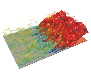
  $\boldsymbol {\nabla }{\boldsymbol u}$, respectively. It is seen that the flame propagates upstream as time advances, indicating the occurrence of boundary layer flashback. There are complex interactions between the flame front and boundary layer turbulence. The flame is rather wrinkled by boundary layer turbulence, and turbulence is also modified by the flame, where backflow regions with negative streamwise velocity are observed.

Figure 6. Temporal evolution of the premixed flame with the instantaneous distribution of the flame front (represented by red isosurface) and the backflow region (represented by blue isosurface). The boundary layer turbulence (characterized by  $\lambda _2=-6\,{\rm s}^{-1}$) is shown and coloured by streamwise velocity; (a) $\text {Time} = 0.21\tau _f$, (b) $\text {Time} = 0.435\tau _f$, (c) $\text {Time} = 0.66\tau _f$, (d) $\text {Time} = 0.90\tau _f$, (e) $\text {Time} = 1.14\tau _f$, ( f) $\text {Time} = 1.38\tau _f$.
The instantaneous distribution of the flame front and vortical structures in an enlarged region is shown in figure 7. It is clear that the backflow regions are located upstream of the flame bulges that are convex towards the reactants, which was also observed in previous studies (Heeger et al. Reference Heeger, Gordon, Tummers, Sattelmayer and Dreizler2010; Eichler & Sattelmayer Reference Eichler and Sattelmayer2012; Gruber et al. Reference Gruber, Chen, Valiev and Law2012; Ebi & Clemens Reference Ebi and Clemens2016; Schneider & Steinberg Reference Schneider and Steinberg2020). The wrinkling of the flame is characterized by the flame curvature  $\boldsymbol {\nabla } \boldsymbol {\cdot } {\boldsymbol n}$, which is positive (negative) when the curvature centre is in the products (reactants), where ${\boldsymbol n}$ is the flame-normal vector defined as ${\boldsymbol n}=-\boldsymbol {\nabla } c /|\boldsymbol {\nabla } c|$. It can be seen that positive curvature is dominant as the flame propagates upstream.

Figure 7. The instantaneous distribution of the flame front (represented by red isosurface) and the backflow region (represented by blue isosurface). The boundary layer turbulence (characterized by  $\lambda _2=-6\,{\rm s}^{-1}$) are shown and coloured by streamwise velocity.
In the following, the displacement speed of the flame front and its components are analysed and compared with the flow velocity in the flame-normal direction to quantify the boundary layer flashback behaviour. The displacement speed of the flame front  $S_d$ is defined as (Chen & Im Reference Chen and Im1998)
 \begin{equation} S_d=\frac{1}{\boldsymbol{\nabla} c}\frac{{\rm D} c}{{\rm D} t}=\frac{\dot\omega_c}{\rho |\boldsymbol{\nabla} c|}+\frac{1}{\rho |\boldsymbol{\nabla} c|}\frac{\partial}{\partial x_i} \left(\rho D_c \frac{\partial c}{\partial x_i}\right), \end{equation}
where  $\dot \omega _c$ and $D_c$ are the reaction rate and the mass diffusivity of the progress variable, respectively. The parameter $S_d$ can be further decomposed into three components as (Wang, Hawkes & Chen Reference Wang, Hawkes and Chen2017a; Wang et al. Reference Wang, Hawkes, Chen, Zhou, Li and Aldén2017b)
 \begin{equation} S_d= \underbrace{\frac{\dot\omega_c}{\rho |\boldsymbol{\nabla} c|}}_{S_{d,r}} \underbrace{+\frac{1}{\rho |\boldsymbol{\nabla} c|}\frac{\partial}{\partial n} \left(\rho D_c \frac{\partial c}{\partial n}\right)}_{S_{d,n}} \underbrace{-D_c\boldsymbol{\nabla} \boldsymbol{\cdot} {\boldsymbol n}}_{S_{d,c}}, \end{equation}
where  $S_{d,r}$, $S_{d,n}$ and $S_{d,c}$ are the reaction, normal diffusion and curvature components, respectively. The flame displacement speed is weighted by density to account for the thermal expansion effects across the flame as $S_d^*=\rho S_d/\rho _u$, where $\rho _u$ is the density of the reactants. The boundary layer flashback is a consequence of the competition between the flame displacement speed $S_d$ and the flow velocity in the flame-normal direction ${\boldsymbol u}\boldsymbol {\cdot } {\boldsymbol n}$. Therefore, a flashback speed is introduced in the present work, which is defined as $S_f = S_d+{\boldsymbol u}\boldsymbol {\cdot } {\boldsymbol n}$. Note that the concept of $S_f$ is consistent with the absolute flame speed relative to the laboratory frame (Poinsot & Veynante Reference Poinsot and Veynante2005). According to the definition, when the flame displacement speed $S_d$ is balanced by the flow velocity in the flame-normal direction, i.e. $S_f = S_d+{\boldsymbol u}\boldsymbol {\cdot } {\boldsymbol n} = 0$, the flame appears statistically stationary in the laboratory coordinate system; when $S_f > 0$ ( $S_f < 0$), the flame propagates upstream (retreats downstream).
Figure 8 shows the normalized density-weighted displacement speed and its components, flow velocity in the flame-normal direction and flashback velocity conditionally averaged on the flame front as a function of the wall-normal distance  $y^+$. The results of the conditional mean curvature are also plotted. Here, the displacement speed is estimated on the isosurface of $c=0.7$, which corresponds to the location of the maximum heat release rate.

Figure 8. Conditional means as a function of normalized wall-normal distance  $y^+$ of the following quantities: $S_d^*/S_L$, $S_{d,r}^*/S_L$, $S_{d,n}^*/S_L$, $S_{d,c}^*/S_L$, $-({\boldsymbol u}\boldsymbol {\cdot } {\boldsymbol n})^*/S_L$, $S_f^*/S_L$ and $(\boldsymbol {\nabla } \boldsymbol {\cdot } {\boldsymbol n})\delta _L$.
It can be seen that the value of  $S_d^*/S_L$ is non-zero at $y^+=0$, although the reaction rate of hydrogen is negligible near the wall due to the low wall temperature. The conditional mean of $S_d^*/S_L$ first increases with increasing $y^+$, and then levels off in the logarithmic region ( $y^+>30$), approaching unity. The findings are consistent with the flame speed analysis reported by Gruber et al. (Reference Gruber, Chen, Valiev and Law2012). To better understand the behaviour of the displacement speed, its components are also analysed. As can be seen, the conditional mean of the reaction component $S_{d,r}^*$ is zero at the wall, confirming that the reaction of hydrogen can be neglected. The conditional mean of $S_{d,r}^*$ increases with increasing wall-normal distance before reaching its peak around $y^+=10$, then it decreases and plateaus around $y^+=30$. As mentioned earlier, lean hydrogen combustion is susceptible to thermo-diffusive instability. Figure 8 shows that positive curvature dominates in the buffer layer and has a maximum value at $y^+=10$, which corresponds to the flame bulges that are convex towards the reactants in the near-wall region, as shown in figure 7. Therefore, the hydrogen reaction is enhanced at positively curved regions, resulting in the peak of $S_{d,r}^*$ near $y^+=10$. In contrast, a local minimum of the normal diffusion and curvature components occurs at $y^+=10$, which is correlated with the local maximum curvature. Away from the wall with large values of $y^+$, the mean curvature is near zero and the flame speed is close to the laminar value. Overall, the reaction component is dominant over the normal diffusion and curvature components, resulting in a positive displacement speed. It is also found that the conditional mean of $S_f^*$ is positive for all values of $y^+$, which indicates the flame propagates upstream and the flame flashback occurs.
Figure 9 shows the density-weighted  $S_d$, ${\boldsymbol u}\boldsymbol {\cdot } {\boldsymbol n}$ and $S_f$ conditioned on $\boldsymbol {\nabla } \boldsymbol {\cdot } {\boldsymbol n}$ and the probability density function (p.d.f.) of $\boldsymbol {\nabla } \boldsymbol {\cdot } {\boldsymbol n}$. The statistics are collected in the buffer layer, i.e. $5< y^+<30$ and conditioned on the flame front. It is clear that the p.d.f. of curvature is positively skewed, and positive curvature of the flame front is dominant in the buffer layer, which is consistent with the observed flame bulges in the near-wall region, as shown in figure 7. The displacement speed is negatively correlated with curvature, which was also observed in previous DNS results (Chakraborty & Cant Reference Chakraborty and Cant2005) for turbulent flames with low Lewis numbers. The conditional mean of the flow velocity in the flame-normal direction is positively correlated with curvature, which is explained as follows. As shown in figure 7, the backflow regions are ahead of flame bulges with positive curvature. The probability of finding positive values of ${\boldsymbol u}\boldsymbol {\cdot } {\boldsymbol n}$ is higher at flame bulges, which results in an increased value of ${\boldsymbol u}\boldsymbol {\cdot } {\boldsymbol n}$ with increasing $\boldsymbol {\nabla } \boldsymbol {\cdot } {\boldsymbol n}$. However, ${\boldsymbol u}\boldsymbol {\cdot } {\boldsymbol n}$ is overall negative as the mean flow direction is misaligned with the mean flame-normal direction. Finally, it is seen that the flashback speed, $S_f$, is higher in positively curved regions than in negatively curved regions. Therefore, the flame flashback is faster in regions with positive curvatures, consistent with the observations in figure 7. Overall, the DNS results showed that backflow regions are ahead of flame bulges, which impacts the flashback behaviours of the boundary layer flame. In the following, the mechanism of the occurrence of backflow is explored.

Figure 9. Normalized density-weighted  $S_d$, $S_f$ and ${\boldsymbol u}\boldsymbol {\cdot } {\boldsymbol n}$ conditionally averaged on the flame curvature in the buffer layer. The blue line denotes the p.d.f. of the normalized curvature.
3.2. Budget analysis of the pressure transport equation
Combustion in the boundary layer may result in an adverse pressure gradient ( ${\rm d} p/{\rm d} x>0$), which can potentially lead to flow separation or backflow (Lee & T'ien Reference Lee and T'ien1982; Gruber et al. Reference Gruber, Chen, Valiev and Law2012; Lieuwen Reference Lieuwen2012). The occurrence of backflow in the present study was already discussed in § 3.1, and in this section, this phenomenon is further scrutinized. To investigate the general characteristics of the increase of pressure leading to the flow separation, a 2-D laminar case with flashback is simulated. In this case, the boundary layer thickness is $\delta =0.5$ mm, which is larger than that of the 2-D laminar case as described in § 2, promoting the occurrence of flame flashback. The instantaneous distribution of pressure upstream of a flame bulge for the 2-D laminar case with flame flashback is shown in figure 10. The backflow region and the heat release rate are indicated by the black dashed and red solid isolines, respectively. The streamlines are also displayed. It is seen that the streamlines are reversed in the backflow region, while they are lifted upward in the region above the leading edge. The pressure increases at the leading edge of the flame bulge, resulting in an adverse pressure gradient with ${\rm d} p/{\rm d} x>0$, which was also reported in previous studies (Lee & T'ien Reference Lee and T'ien1982; Eichler & Sattelmayer Reference Eichler and Sattelmayer2012; Gruber et al. Reference Gruber, Chen, Valiev and Law2012). The occurrence of the backflow region is related to the adverse pressure gradient (Gruber et al. Reference Gruber, Chen, Valiev and Law2012). The underlying mechanism of the appearance of adverse pressure gradients ahead of flame bulges is not well understood from the literature. Gruber et al. (Reference Gruber, Chen, Valiev and Law2012) suggested that Darrieus–Landau hydrodynamic instability (Williams Reference Williams1985) plays a critical role in the formation of the backflow region and affects the near-wall pressure field. In the present study, the pressure behaviour is investigated by analysing the budget terms of the pressure transport equation, which is derived by substituting the state equation, $p=\rho RT$, into the conservation equation for energy (see Appendix A for the derivation). The final form of the pressure transport equation is written as
 \begin{align} \frac{\partial p}{\partial t}=& \underbrace{-u_i\frac{\partial p}{\partial x_i}}_{T0} \underbrace{-\gamma p\frac{\partial u_i}{\partial x_i}}_{T1} \underbrace{+\frac{R}{C_v}\dot \omega_T}_{T2} \underbrace{+\frac{R}{C_v}\frac{\partial}{\partial x_i}\left(\lambda \frac{\partial T}{\partial x_i}\right)}_{T3}\nonumber\\ &\quad \underbrace{-\frac{R}{C_v}\left(\rho \sum_{k=1}^N V_{k,i}Y_k C_{p,k}\frac{\partial T}{\partial x_i}\right)}_{T4} \underbrace{+\frac{R}{C_v}\tau_{ij}\frac{\partial u_i}{\partial x_j}}_{T5}, \end{align}
where  $\gamma$ is the ratio of the constant pressure specific heat $C_p$ to the constant volume specific heat $C_v$, $R$ is the ideal gas constant, $\dot \omega _T$ is the heat release rate, $\lambda$ is the thermal conductivity, $V_{k,i}$ is the species diffusion velocity in the $i$th direction for the $k$th species, $N$ is the number of species, $Y_k$ is the mass fraction of the $k$th species and $\tau _{ij}$ is the viscous tensor. The terms on the right-hand side of the equation are the convection term ( $T0$), dilatation term ( $T1$), reaction term ( $T2$), thermal diffusion term ( $T3$), species diffusion term ( $T4$) and viscous term ( $T5$).

Figure 10. Instantaneous distribution of normalized pressure in an  $x$–
$x$– $y$ plane with a flame bulge for the 2-D case with flashback. The white lines indicate the streamlines. The black dashed line and red isolines denote the backflow region and the heat release rate, respectively. The black solid line is used to extract the budget terms of the pressure transport equation. The length of the black line is 0.4 mm.
For the 2-D laminar case with flashback, the budget terms of the pressure transport equation along the solid black line in figure 10 are analysed and the profiles are shown in figure 11. The black solid line is chosen so that it is aligned with the flame-normal direction, which captures the evident variations of the pressure and its budget terms. The transient term,  $\partial p/\partial t$, is the sum of $T0$ to $T5$. As can be seen, the dilatation term ( $T1$), reaction term ( $T2$) and thermal diffusion term ( $T3$) are the main contributors to the pressure variation, while the species diffusion term and viscous term are negligible in the region of interest. Near the location of the maximum pressure, it is found that the positive thermal diffusion term is dominant over the dilatation term and reaction term, which results in a net positive value on the right-hand side of (3.3). Therefore, the pressure increases and reaches its maximum. It is interesting to see from an enlarged region in figure 11(b) that, on the reactant side with small values of $x$, the dilatation term is positive and is roughly balanced by the negative thermal diffusion term. Close to the product side with large values of $x$, it is observed that both the dilatation term and reaction term are negative and large, which results in a net reduction of the pressure. From the above analysis, it is concluded that the positive thermal diffusion term and dilatation term near the leading edge of the flame bulge are responsible for the increase of pressure, resulting in the observed adverse pressure gradient and backflow.

Figure 11. Budget terms of the pressure transport equation extracted from the black line in figure 10.
The characteristics of pressure in the more complex 3-D turbulent case are presented. Figure 12(a) shows the top view of the 3-D turbulent boundary layer flashback. It can be seen the flame is rather wrinkled in the spanwise direction. Similar observations were also made by Gruber et al. (Reference Gruber, Chen, Valiev and Law2012, Reference Gruber, Kerstein, Valiev, Law, Kolla and Chen2015), and it was concluded that the initial wrinkling of the flame surface is triggered by the boundary layer streak structure. In addition, the backflow regions exist upstream of flame bulges. The distributions of pressure and its transport budget terms of the 3-D turbulent case are examined in a typical  $x$–
$x$– $z$ plane in the buffer region ( $y^+\approx 27$ with $y=0.348$ mm), and are shown in figure 12(b–h). The isolines of $c=0.01$ and $c=0.7$ are indicated by dashed and solid black isolines, respectively. It is noted that the pressure is high in front of the upstream flame bulges that are convex towards the reactants, while it is low in the downstream cusps of the flame that are convex towards the products. The contours of pressure budget terms indicate that $T1$,
$T1$,  $T2$ and $T3$ are the main contributors to pressure change. The values of $T1$ and $T2$ are generally negative, while the value of $T3$ is positive.

Figure 12. Instantaneous contours of (a) flame front and  $\lambda _2$ vortex, (b) normalized pressure and (c–h) budget terms of the pressure transport equation in an $x$–
$x$– $z$ plane. The dashed and solid black lines in (b–h) denote the isosurfaces of $c=0.01$ and $c=0.7$, respectively. The red solid line indicates the isoline of $u=0\,{\rm m}\,{\rm s}^{-1}$ (backflow region); (b) $p/p_0$, (c) $T_0$, (d) $T_1$, (e) $T_2$, ( f) $T_3$, (g) $T_4$, (h) $T_5$.
Figure 13 shows the instantaneous distribution of normalized pressure in a typical  $x$–
$x$– $y$ plane for the 3-D turbulent case. It is interesting to see that the distribution of the pressure is similar to that for the 2-D laminar case with flashback, as shown in figure 10. To evaluate the contributions of various terms of the pressure transport equation in the 3-D turbulent case, the profiles of the pressure budget terms extracted from the black lines of figure 13 are displayed in figure 14. As can be seen, the trends of various terms are not sensitive to the choice of the lines. It is noted that the variation of pressure is more complex compared with the 2-D laminar case. Consistent with the scenario in the 2-D laminar case, the positive dilatation term ( $T1$) and thermal diffusion term ( $T3$) are responsible for the increase of pressure in front of the flame, which results in the adverse pressure gradient.

Figure 13. Instantaneous distribution of normalized pressure in a typical  $x$–
$x$– $y$ plane with a flame bulge for the 3-D case. The white lines indicate the streamlines. The black dashed line and red isolines denote the backflow region and the heat release rate, respectively. Three lines are used to extract the budget terms of the pressure transport equation. The value of wall-normal distance is $y^+ =18$, 24 and 30 mm for lines A, B and C, respectively.

Figure 14. Budget terms of the pressure transport equation extracted from the black lines in figure 13: (a) line A, (b) line B and (c) line C.
3.3. The effects of combustion on turbulent boundary layer
The flame-induced adverse pressure gradient leads to the local boundary layer separation (backflow regions) in front of the flame bulges towards the reactants and affects the flow structures, which can be understood by examining the velocity profiles. The mean streamwise velocity  $\bar {u}^+$ along the wall-normal distance $y^+$ at the time instant of $0.825 \tau _f$ is shown in figure 15. Note that the mean streamwise velocity is computed using samples in the spanwise direction. The most upstream location of the mean flame for this timing is at $x=11.8$ mm. It is noted that, in the near-wall region, the mean streamwise velocity is lower than the non-reacting case in front of the flame ( $x=8$ mm), which means the streamwise velocity is reduced by the adverse pressure gradient in front of the flame. Due to the flow acceleration by thermal effects, the mean velocity profile at $x=11.8$ mm is higher than that in the non-reacting case in the viscous sublayer. In the downstream region ( $x=13$ mm), the mean velocity is higher than that in the non-reacting case in the viscous sublayer and buffer region.

Figure 15. The profiles of mean streamwise velocity along the wall-normal distance for the reacting and non-reacting cases. The average is conditioned on the spanwise direction for the reacting case and time is  $0.825\tau _f$. The average is conditioned on time and the spanwise direction for the non-reacting case.
The boundary layer separation and reattachment along the streamwise direction can impact the mean skin-friction coefficient  $C_f$ (Spalart & Watmuff Reference Spalart and Watmuff1993; Aubertine & Eaton Reference Aubertine and Eaton2005), which is given as
 \begin{equation} C_f = \frac{\tau_w}{\frac{1}{2}\rho_wU_\infty^2} = \frac{\mu \dfrac{{\rm d}\bar{u}}{{\rm d} y}|_{y=0}}{\frac{1}{2}\rho_wU_\infty^2}, \end{equation}
where  $\tau _w$ is the mean wall stress, $\rho _w$ is the density of the reactants at the height of $y=0$ and $U_\infty$ is the inflow free-stream velocity. Figure 16 shows the distributions of mean skin-friction coefficient $C_f$ along the streamwise direction for the reacting and non-reacting cases. As can be seen, in the non-reacting case, $C_f$ is around $4.5\times 10^{-3}$ along the streamwise direction. Note that, although the non-reacting case is a spatially evolving turbulent boundary layer, the spatial development of the boundary layer turbulence is slow, so that the statistics of various quantities do not vary evidently in the streamwise direction of the computational domain. Therefore, the value of $C_f$ can be regarded as constant along the streamwise direction. This value is close to that for a zero-pressure-gradient fully developed boundary layer flow in Li, Luo & Fan (Reference Li, Luo and Fan2016). In the reacting case, the distributions of $C_f$ decrease with $x$, reach a negative minimum value around the reacting region and then increase on the product side. In front of the reaction region, the flame-induced adverse pressure gradient leads to the boundary layer separation and low mean streamwise velocity near the wall, which results in a small value of $\tau _w$ and $C_f$. While on the product side, combustion dilatation accelerates the mean streamwise velocity, contributing to the increase of $\tau _w$ and $C_f$, and the boundary layer reattaches to the wall.

Figure 16. The profiles of mean skin-friction coefficient  $C_f$ along the streamwise direction for the reacting and non-reacting cases. The average is conditioned on the spanwise direction for the reacting case, and on time and the spanwise direction for the non-reacting case.
To further understand the flame–flow interactions, the influence of the flame-induced adverse pressure gradient on the turbulent boundary layer vortical structures is investigated. Figure 17 shows the coherent vortical structures of the turbulent boundary layer, which are represented by the  $\lambda _2=-6\,{\rm s}^{-1}$ isosurface and coloured by the streamwise velocity for both the reacting and non-reacting cases. The flame front of the reacting case is also shown. The data of visualization are extracted from the same time instant for the two cases. The classical boundary layer turbulent structures with hairpin vortices are observed for both cases in figure 17. Comparing the results of the two cases, it is noted that the vortical structures are lifted in the reacting case near and downstream of the backflow region, with the angle between the coherent vortical structures and the wall-normal vector ${\boldsymbol n}_{wall}$ being obviously smaller in the reacting case than that in the non-reacting case. The orientations of coherent vortical structures are further quantified in the following.

Figure 17. Instantaneous contours of turbulent boundary layer coherent vortical structures (represented by  $\lambda _2=-6\,{\rm s}^{-1}$ isosurface and coloured by streamwise velocity) for the (a) reacting and (b) non-reacting cases. The red isosurface denotes the flame front (represented by $c=0.7$).
Figure 18 shows a schematic of vortex filaments in boundary layer turbulence, where two characteristic angles are defined, including the elevation angle ( $\theta _e$), i.e. the angle formed with the wall plane, and the projection angle ( $\theta _{zx}$) in the wall plane. Obviously, the elevation angle varies from $-{\rm \pi} /2$ to ${\rm \pi} /2$, and the projection angle from $-{\rm \pi}$ to ${\rm \pi}$. By convention, the projection angle is measured with respect to the positive $z$ direction. The statistics of the characteristic angles are examined in terms of the p.d.f. and it is worth noting that, for an isotropic distribution of a unit vector, the p.d.f. of the elevation angle $P(\theta _e)$ is $\cos \theta _e/2$ and that of the projection angle $P(\theta _{zx})$ is $1/2{\rm \pi}$ (Wang et al. Reference Wang, Hawkes, Ren, Chen, Luo and Fan2021a). To avoid biasing towards small values of $\theta _e$, a scaled p.d.f. for $\theta _e$ is introduced (Pirozzoli, Bernardini & Grasso Reference Pirozzoli, Bernardini and Grasso2008)
 \begin{equation} \tilde{P}(\theta_e)=\frac{P(\theta_e)/{\cos}\theta_e}{\int_{-{\rm \pi}/2}^{{\rm \pi}/2} P(\theta_e)/{\cos}\theta_e \,{\rm{d}}\theta_e} \end{equation}
which yields  $\tilde {P}(\theta _e) = 1/{\rm \pi}$ for an isotropic distribution of a unit vector. In the present study, coherent vortical structures are identified in regions where the magnitude of $\lambda _2$ exceeds a suitable threshold. Although not shown here, this threshold results in similar vortices as those using the threshold by Pirozzoli et al. (Reference Pirozzoli, Bernardini and Grasso2008). Once the vortical structures are educed, the p.d.f.s of characteristic angles using the $\boldsymbol \omega$-criterion are calculated, where ${\boldsymbol \omega }$ is the vorticity vector.

Figure 18. Schematic of vortex filaments in boundary layer turbulence.
The p.d.f.s of  $\theta _e$ and $\theta _{zx}$ are displayed in figure 19. The DNS results from a supersonic turbulent boundary layer by Pirozzoli et al. (Reference Pirozzoli, Bernardini and Grasso2008) are also shown for comparison. It is seen that the p.d.f. of $\theta _e$ in the present work is in a good agreement with that in Pirozzoli et al. (Reference Pirozzoli, Bernardini and Grasso2008). Particularly, the p.d.f. peaks near $\theta _e = \pm 45^\circ$ in both studies, confirming the existence of hairpin vortices. The probability is the lowest when $\theta _e = \pm 90^\circ$. As for the p.d.f. of $\theta _{zx}$, it is seen that the probability is the lowest when $\theta _{zx} = 0^\circ$ in both studies. However, the peak of the p.d.f. in the present study is near $\theta _{zx} = \pm 90^\circ$ while that in Pirozzoli et al. (Reference Pirozzoli, Bernardini and Grasso2008) is near $\theta _{zx} = \pm 60^\circ$. Figure 20 compares the p.d.f.s of $\theta _e$ and $\theta _{zx}$ for the non-reacting and reacting cases. As can be seen, the p.d.f.s of $\theta _{zx}$ are very similar between the two cases. However, the p.d.f.s of $\theta _{e}$ are considerably different. Specifically, in the reacting case, the elevation angle is generally larger than that in the non-reacting case, so that the probability of finding large values of $\theta _{e}$ is higher for the reacting case. The results are consistent with the visualization of boundary layer turbulence in figure 17, where the coherent vortical structures are lifted in the reacting case.

Figure 19. The p.d.f.s of the characteristic angles for the non-reacting case: (a)  $\theta _e$ and (b) $\theta _{zx}$ in the logarithmic region. The DNS results of Pirozzoli et al. (Reference Pirozzoli, Bernardini and Grasso2008) are also included.

Figure 20. The p.d.f.s of the characteristic angles for the non-reacting and reacting cases: (a)  $\theta _e$ and (b) $\theta _{zx}$ in the logarithmic region.
The effects of combustion on the boundary layer turbulence are further examined based on the sign of velocity fluctuations in the Reynolds stress component  $\overline {u^\prime v^\prime }$. Four events, i.e. Q1 ( $u^\prime >0$, $v^\prime >0$), Q2 ( $u^\prime <0$, $v^\prime >0$), Q3 ( $u^\prime <0$, $v^\prime <0$) and Q4 ( $u^\prime >0$, $v^\prime <0$), can be identified (Willmarth & Lu Reference Willmarth and Lu1972; Krogstad & Skåre Reference Krogstad and Skåre1995), where Q1 and Q3 indicate the outward and inward interactions, respectively, while Q2 and Q4 correspond to the ejection and sweep events, respectively (Willmarth & Lu Reference Willmarth and Lu1972). Note that the Q2 event (ejection event) transports low-speed fluid away from the wall, while the Q4 event (sweep event) transports high-speed fluid into the inner layer (Corino & Brodkey Reference Corino and Brodkey1969). Figure 21 shows the fractions of the four events along with $y^+$ for the reacting and non-reacting cases. It can be seen that the total contributions of the ejection and sweep events are comparable in both the reacting and non-reacting cases. However, the fraction of the ejection event is larger than that of the sweep event in the reacting case, while the fractions of the two events are similar in the non-reacting case. The fraction of the ejection event (sweep event) is higher (lower) for the reacting case than that for the non-reacting case across the boundary layer. The suppression of the sweep event in the reacting case leads to an extension of the low-velocity regions in the near-wall region, which facilitates the occurrence of the boundary layer flashback.

Figure 21. Fractions of different events along with the wall-normal distance. The solid and dashed lines indicate the results from the reacting case and the non-reacting case, respectively.
4. Conclusions
In the present work, DNS of lean hydrogen/air premixed flame flashback in boundary layer turbulence was performed. The characteristics of flame flashback, the underlying mechanisms of the adverse pressure gradient at the leading edge of flame bulges and the effects of combustion on the turbulent boundary layer structures were explored. The main findings are summarized as follows.
First, the features of boundary layer flashback are analysed quantitatively in terms of the flame displacement speed  $S_d$, and the role of curvature on the flame flashback is revealed. The displacement speed has been decomposed into various components to understand the boundary layer flashback behaviours. It was shown that thermo-diffusive instability plays an important role in the present lean hydrogen/air premixed flame so that the reaction component of the displacement speed is larger in flame bulges with positive curvature. A flashback speed defined as $S_f = S_d + {\boldsymbol u}\boldsymbol {\cdot } {\boldsymbol n}$ is used to characterize the flame flashback, which is also larger in regions with positive curvature due to the existence of backflow.
Second, the backflow phenomenon is related to the flame-induced adverse pressure gradient in the flow. The mechanism of adverse pressure gradient was, for the first time, explored through the analysis of the pressure transport equation, which showed that the positive dilatation and thermal diffusivity terms near the leading edge of flame bulges are the main reason for the increase of pressure, and the resultant adverse pressure gradient. The trends of various terms are not sensitive to the choice of the wall-normal location.
Finally, the influence of combustion on the boundary layer turbulence was examined. The mean streamwise velocity and skin-friction coefficient are damped by the flame-induced adverse pressure gradient. It was found that the turbulent boundary layer coherent vortical structures are lifted near and downstream of the backflow region, which was quantified using the elevation angle of the vorticity vector. It was shown that the elevation angle is generally larger in the reacting case than that in the non-reacting case. Four events based on the analysis of the Reynolds stress component  $\overline {u^\prime v^\prime }$ were studied, and it was shown that the ejection event is stronger due to combustion while the sweep event is weaker, which facilitates the occurrence of flame flashback.
Funding
This work was supported by the National Natural Science Foundation of China (Grant Nos. 51836007, 52022091 and 51976185) and the Fundamental Research Funds for the Central Universities (Grant No. 2021FZZX001-10).
Declaration of interests
The authors report no conflict of interest.
Appendix A. Transport equation for pressure
The conservation equation for energy in the temperature form is written as (Poinsot & Veynante Reference Poinsot and Veynante2005)
 \begin{equation} \rho{C_p}\frac{{\mathrm D}{T}}{{\mathrm D}t} = {\dot \omega}_T+\frac{{\mathrm D}p}{{\mathrm D}t}+\frac{\partial}{\partial x_i}\left(\lambda \frac{\partial T}{\partial x_i}\right)-\rho\sum_{k=1}^{N}V_{k,i}Y_k C_{p,k} \frac{\partial T}{\partial x_i}+\tau_{ij}\frac{\partial u_i}{x_j}, \end{equation}
where  ${{\mathrm D}T}/{{\mathrm D}t}={\partial T}/{\partial t}+u_i{\partial T}/{\partial x_i}$ and ${{\mathrm D}p}/{{\mathrm D}t}={\partial p}/{\partial t}+u_i{\partial p}/{\partial x_i}$. Alternatively, the equation can also be expressed as
 \begin{equation} \rho{C_p}\frac{{\mathrm D}{T}}{{\mathrm D}t}-\frac{{\mathrm D}p}{{\mathrm D}t} = {\dot \omega}_T+\frac{\partial}{\partial x_i}\left(\lambda \frac{\partial T}{\partial x_i}\right)-\rho\sum_{k=1}^{N}V_{k,i}Y_k C_{p,k} \frac{\partial T}{\partial x_i}+\tau_{ij}\frac{\partial u_i}{x_j}. \end{equation}
Using the state equation  ${p = \rho RT}$, the following relationship is derived:
 \begin{equation} \frac{{\mathrm D}{p}}{{\mathrm D}t} = RT\frac{{\mathrm D}{\rho}}{{\mathrm D}t} + R\rho\frac{{\mathrm D}{T}}{{\mathrm D}t} ={-}p\frac{{\partial u_i}}{{\partial x_i}} + R\rho\frac{{\mathrm D}{T}}{{\mathrm D}t}. \end{equation}
Therefore
 \begin{equation} \rho{C_p}\frac{{\mathrm D}{T}}{{\mathrm D}t} = \frac{C_p}{R}\frac{{\mathrm D}{p}}{{\mathrm D}t}+\frac{C_p}{R}p\frac{{\partial u_i}}{{\partial x_i}}. \end{equation}
Subtracting  ${\mathrm D}{p}/{\mathrm D}t$ from both sides of (A4), we obtain
 \begin{equation} \rho{C_p}\frac{{\mathrm D}{T}}{{\mathrm D}t} - \frac{{\mathrm D}{p}}{{\mathrm D}t} = \frac{C_v}{R}\frac{{\mathrm D}{p}}{{\mathrm D}t}+\frac{C_p}{R}p\frac{{\partial u_i}}{{\partial x_i}} = \frac{C_v}{R}\left(\frac{{\mathrm D}{p}}{{\mathrm D}t} + \gamma{p}\frac{{\partial u_i}}{{\partial x_i}}\right). \end{equation}
Combining (A2) and (A5), the following is obtained:
 \begin{equation} \frac{C_v}{R}\left(\frac{{\mathrm D}{p}}{{\mathrm D}t} + \gamma{p}\frac{{\partial u_i}}{{\partial x_i}}\right) = {\dot \omega}_T+\frac{\partial}{\partial x_i}\left(\lambda \frac{\partial T}{\partial x_i}\right)-\rho\sum_{k=1}^{N}V_{k,i}Y_k C_{p,k} \frac{\partial T}{\partial x_i}+\tau_{ij}\frac{\partial u_i}{x_j}. \end{equation}
Finally, the transport equation for pressure is expressed as
 \begin{align} \frac{\partial p}{\partial t}+u_i\frac{\partial p}{\partial x_i}+\gamma{p}\frac{\partial u_i}{\partial x_i} = \frac{R}{C_v}{\dot \omega}_T+\frac{R}{C_v}\frac{\partial}{\partial x_i}\left(\lambda \frac{\partial T}{\partial x_i}\right)-\frac{R}{C_v}\rho\sum_{k=1}^{N}V_{k,i}Y_k C_{p,k} \frac{\partial T}{\partial x_i}+\frac{R}{C_v}\tau_{ij}\frac{\partial u_i}{x_j}. \end{align}


