


1. Introduction
For almost four decades up to the 1990s, high-redshift radio galaxies were the most distant galaxies known (Stern & Spinrad Reference Stern and Spinrad1999). Since the advent of deep optical surveys and the dropout technique (e.g. Steidel et al. Reference Steidel, Adelberger, Giavalisco, Dickinson and Pettini1999), other selection techniques have overtaken radio, finding both the largest numbers and the most distant galaxies. The stiff competition from optical surveys has also slowed down the search for the most distant radio galaxies; while the radio galaxy TN J0924-2201 was the second most distant galaxy known at the time of its discovery ( $z=5.19$ van Breugel et al. Reference van Breugel, De Breuck, Stanford, Stern, Röttgering and Miley1999), it was quickly overtaken by many optically selected galaxies. It remained the most distant radio-selected galaxy known for two decades until the discovery of TGSS J1530+1049 at
  $z=5.72$ (Saxena et al. Reference Saxena2018b). However, this radio galaxy is less luminous than the bulk of the classical powerful radio galaxies (Miley & De Breuck Reference Miley and De Breuck2008). While TGSS J1530+1049 may represent a larger population at these redshifts, the more luminous radio galaxies are important to study in their own right. Decades of research have demonstrated that the most powerful high-redshift radio galaxies are hosted by massive galaxies (Seymour et al. Reference Seymour2007; De Breuck et al. Reference De Breuck2010), with the most massive black holes (Nesvadba et al. Reference Nesvadba, Drouart, De Breuck, Best, Seymour and Vernet2017; Drouart et al. Reference Drouart2014) in the most massive dark matter over-densities (Galametz et al. Reference Galametz2012; Mayo et al. Reference Mayo, Vernet, De Breuck, Galametz, Seymour and Stern2012). Furthermore, should a radio galaxy be detected at
  $z>6.5$ it would be possible to search absorption by neutral hydrogen in the Epoch of Reionisation (EoR) against this background source (e.g. Carilli et al. Reference Carilli, Gnedin, Furlanetto and Owen2004; Ciardi et al. Reference Ciardi2015).
It is difficult to find radio-loud active galactic nuclei (AGN) at the highest redshifts because they are both optically faint and intrinsically rare. While wide-field optical surveys are now finding quasars out to  $z=7.5$ (Bañados et al. Reference Bañados2018a), the most distant powerful (
 $L_{\rm 500\,MHz}>10^{27}\,\text{WHz}^{-1}$) radio-loud sources do not currently reach above
  $z\sim 6$ (e.g. McGreer et al. Reference McGreer, Becker, Helfand and White2006; Zeimann et al. Reference Zeimann, White, Becker, Hodge, Stanford and Richards2011; Bañados et al. Reference Bañados, Carilli, Walter, Momjian, Decarli, Farina, Mazzucchelli and Venemans2018b). Most radio-loud AGN are obscured type 2 sources, hence are much harder to find than the bright type 1 (unobscured) AGN. Furthermore, the difficulty in finding such sources is possibly related to the sharp decline in the AGN luminosity function at
  $z>3$ (e.g. Best et al. Reference Best, Ker, Simpson, Rigby and Sabater2014), the reasons for which are not clear.
As powerful radio galaxies at  $z>5$ are so rare, the best way to find them is from the widest surveys. Here, radio surveys still have an advantage over optical surveys, as several of the former have all-sky coverage. The most difficult part of the identification is that these radio surveys contain hundreds of thousands objects, while their redshift determination remains very time consuming and can only be done on a few tens of optimal candidates. It is therefore crucial to have an efficient down-selection directly in the radio. The most popular technique is the selection by means of their ultra-steep radio spectra (e.g. Blumenthal & Miley Reference Blumenthal and Miley1979; Rottgering et al. Reference Rottgering, Lacy, Miley, Chambers and Saunders1994; De Breuck et al. Reference De Breuck, van Breugel, Röttgering and Miley2000, Reference De Breuck, Tang, de Bruyn, Röttgering and van Breugel2002, Reference De Breuck, Hunstead, Sadler, Rocca-Volmerange and Klamer2004; Broderick et al. Reference Broderick, Bryant, Hunstead, Sadler and Murphy2007; Saxena et al. Reference Saxena2018a). This empirical technique relies on the steepening of the observed spectral indices with redshift, which is due to a fixed concave shape and/or an evolution with redshift of the radio spectral shape (e.g. Klamer et al. Reference Klamer, Ekers, Bryant, Hunstead, Sadler and De Breuck2006; Ker et al. Reference Ker, Best, Rigby, Röttgering and Gendre2012). While these ultra-steep spectrum (USS) search techniques have been efficient in finding the most distant radio galaxies, they do offer a biased and incomplete view of the full population of radio-loud AGN as the selection function is not well understood (e.g. Barthel Reference Barthel1989). Another disadvantage of this technique is that it requires observations at two frequencies in surveys that are well matched in spatial resolution and depth.
In this paper, we present results from a pilot survey of powerful high-redshift radio galaxies using the Galactic and Extra-galactic All-sky Murchison Wide-field Array (GLEAM) surveyFootnote a (Wayth et al. Reference Wayth2015) observed with the Murchison Wide-field Array (MWA; Lonsdale et al. Reference Lonsdale2009; Tingay et al. Reference Tingay2013). The main advantage of this survey is that it provides spectral information over a wide bandwidth at low frequencies. Hence, this survey allows one to conduct an efficient selection based on the actual shape of the radio spectral energy distribution (SED), rather than having to rely on a single spectral index. We introduce our new selection technique in Section 2, and then our near-infrared (NIR), the Australian Telescope Compact Array (ATCA) and Atacama Large Millimetre Array (ALMA) follow-up observations in Section 3. In Section 4, we present the first results of our pilot survey. We discuss our results in Section 5, and conclude this paper in Section 6.
2. Defining a sample to select  $\textbf{\textit{z}}\boldsymbol >\textbf{5}$ radio galaxies

The GLEAM survey is an all-sky low-frequency radio survey performed by the MWA, which provides 20 photometric data-points in the 70–230 MHz range. The final resolution is in the 2–6 arcmin range for an average rms noise of  $\sim30\,\text{mJy beam}^{-1}$ at 151 MHz. Sources are detected in a broadband high-resolution image across 170–230 MHz and then flux densities are measured in the 20 8 MHz sub-bands with prioritised positions. The extra-galactic first data release (Hurley-Walker et al. Reference Hurley-Walker2017) contains 307 455 radio components above
  $5\sigma$ with 99.97% reliability. We refer the reader to that paper for a complete description of the data processing, source finding, and catalogue release.
We made our original selection using the third internal data release (IDR3, 2016 March) available to the MWA consortium at that time. Hence, the data in Figure 1 and Table 1 differ a little from the public data of Hurley-Walker et al. (Reference Hurley-Walker2017). These differences are small, but we described them in more detail in Appendix A. Below, we described our selection method.
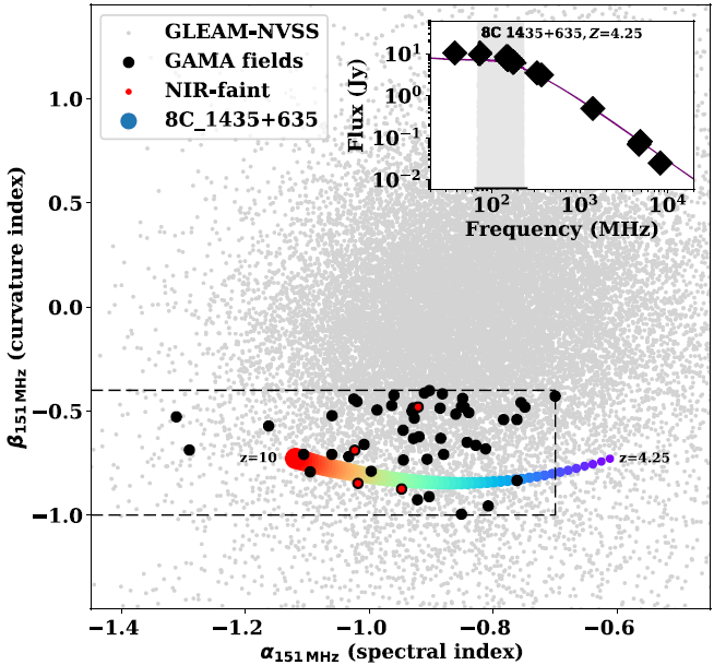
Figure 1. The GLEAM-derived spectral index,  $\alpha$, versus curvature term,
  $\beta$, for our full GLEAM-NVSS matched catalogue (grey points). The dashed lines represent our
  $\alpha\text{/}\beta$ selection criteria. The black points are the 52 sources in the GAMA survey fields and in red, the four high-redshift candidates with faint or no K-band detections in the GAMA 9 h field. The track shows the modelled
  $\alpha\text{/}\beta$ values for the powerful radio galaxy 8C 1435+635 (with its SED presented in the inset) when shifted from its redshift of
  $z=4.25$ up to
  $z=10$. The grey area in the inset corresponds to the GLEAM frequency coverage.
Table 1. Summary of our selection criteria conducted on the IDR3 GLEAM catalogue. Using the public GLEAM release will give slightly different numbers (see Appendix A). See Section 2.3 for more details.
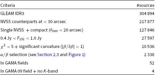
2.1. Isolated and compact sources
We cross-matched the GLEAM catalogue with the NRAO VLA Sky Survey (NVSS; Condon et al. Reference Condon, Cotton, Greisen, Yin, Perley, Taylor and Broderick1998) catalogue using a cross-matching radius of 30 arcsec. The higher resolution of NVSS (45 arcsec) allows us to retain only sources that are relatively compact, with a single component and isolated (no other NVSS component within search radius). We apply a flux density cut of  $0.4\,\text{Jy}<{F}_{\rm 151\,MHz}<1\,\text{Jy}$ in order to (a) remove the brightest sources in the sample (more likely to be at lower redshift and/or extended) and (b) ensure we are only selecting the most powerful radio galaxies at
  $z>5$ as well as maintaining sufficient signal to noise to reliably fit the MWA SED (see Section 2.2).
2.2. MWA SED fitting
We perform a second-order polynomial fit in log space to the GLEAM data, following the equation:
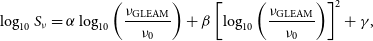 \begin{equation}{\rm log}_{10}\,S_{\nu} = \alpha\,{\rm log}_{10} \left(\frac{\nu_{\rm GLEAM}}{\nu_{0}}\right) + \beta\left[{\rm log}_{10} \left(\frac{\nu_{\rm GLEAM}}{\nu_{0}}\right)\right]^2 + \gamma,\end{equation}
where  $S_{\nu}$ is the flux density in each sub-band,
  $\nu_{\rm GLEAM}$ is the corresponding central frequency,
  $\nu_{0}$ is the central frequency of the total GLEAM frequency coverage (151 MHz), and
  $\alpha,\beta,\gamma$ are the coefficients of the polynomial terms:
  $\alpha$ for the spectral index and
  $\beta$ for the curvature term. The re-normalisation with
  $\nu_{0}$ permits a curvature estimate within the GLEAM frequency range (70–230 MHz). We note that a fraction of the sources are better represented by a first-order polynomial (better
  $\chi^2$). However, in the particular case of power-law spectra, the curvature (
 $\beta$) for these sources will be close to zero and is filtered out during the spectral selection (see next sub-section).
2.3. Spectral selection
In order to further optimise our selection, we make use of the knowledge of one of the largest sample of powerful high-redshift radio galaxies to date. A significant fraction of the sources at  $z>3.5$ in the ‘HeRGÉ’ sample (Seymour et al. Reference Seymour2007; De Breuck et al. Reference De Breuck2010) present a flattening in their radio SED when moving to the lowest frequencies (Drouart et al. in prep). We use one of these sources, 8C 1435+635 (at
  $z=4.25$ see the inset in Figure 1) to predict the
  $\alpha$ and
  $\beta$ at higher redshift (coloured line in Figure 1). We see that the track passes through the
  $-1.0<\beta<-0.4$ region and generally presents a steep spectral index with
  $\alpha<-0.7$ (expected as the sources in the HeRGÉ sample were selected for their steep spectrum and radio luminosity). We therefore isolate this part of the parameter space to select our candidates. We also apply the criteria of
  $\chi^2<5$ and
  $|\beta/\delta\beta|>1$ to ensure that we select source with robust fitting and a significantly curved SED.
2.4. Pilot project on the GAMA 09 field
Finally, we focus on the Galaxy And Mass Assembly (GAMA) survey (Driver et al. Reference Driver2009) where a wealth of multi-wavelength data is available to further isolate the most promising candidates. When considering the 5 GAMA fields together, only 52 sources are left. We visually inspected each source with a JHK image from the VIKING survey (Arnaboldi et al. Reference Arnaboldi, Neeser, Parker, Rosati, Lombardi, Dietrich and Hummel2007). The VIKING  $5\sigma$ sensitivity, mag
  $K_s(\rm AB)=22.1$, is ideally suited to eliminate any lower redshift sources due to the well-established K–z relationship (Rocca-Volmerange et al. Reference Rocca-Volmerange, Le Borgne, De Breuck, Fioc and Moy2004) for powerful radio galaxies. After isolating sources which present no, or very faint NIR, counterparts within a few arc-seconds of the GLEAM position, and restricting ourselves to the GAMA 9 h field (hereafter G09) in order to optimise our ALMA follow-up, we are left with four high-z candidates (see Table 2).
Table 2. Summary of our candidate high-redshift radio galaxies including original IDR3 name, final GLEAM name (both preceded by ‘GLEAM’), short name for this paper, IDR3 151 MHz flux density, and the best fit  $\alpha/\beta/\chi^2$ parameters using the IDR3 data.
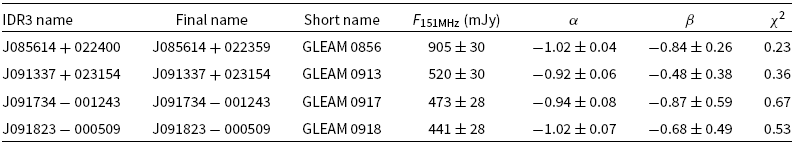
Note the source positions are given by their name with uncertainties of 3–5′′.
To identify the host galaxies, we obtained the following observations: (i) a moderately deep  $K_s$-band imaging with the HAWK-I instrument on the Very Large Telescope (VLT) in order to confirm the location of the host in NIR, not detected in the VIKING data (see Section 3.1), (ii) ATCA continuum imaging at 5.5, 9.0, 17, and 19 GHz to complete the radio SED coverage to over four decades in frequency (see Section 3.2), and (iii) an ALMA Band 3 spectral scan (84–115 GHz, Section 3.3) to obtain simultaneously a deep, sub-arcsecond resolution continuum image to identify the host galaxy in the HAWK-I
  $K_s$ imaging, and to obtain the redshift via the molecular emission lines—the method the South Pole Telescope (SPT) team used for strongly lensed sub-millimetre (sub-mm) galaxies (Weiß et al. Reference Weiß2013; Strandet et al. Reference Strandet2016).
3. Follow-up data
3.1. NIR follow-up observations
Our ESO/HAWK-I programme (0101.A-0571A, PI Drouart) was observed between 2018 April and June in service mode. It consisted of two sets of exposure in  $K_s$-band, centred on CHIP1 (bottom-left quadrant). The total exposure time on each source reaches 1 h. We processed the data with the esorex tool and followed the standard processing recipe described in the HAWK-I manual v2.4.3 for each run. The final mosaics were created using the Montage package v5.0.0 and montage-wrapper v0.9.9 with all options set to their default values. We present the
  $K_s$-band images of our sources in Figure 2. Finally, we perform an aperture photometry based on the positions of host galaxies found in the HAWK-I images and confirmed by the ALMA continuum emission. Flux densities at these positions were extracted from the VIKING zY JHK bands using the phot.utils package v0.5. These flux densities are reported in Table 3 and the resultant SEDs presented in Figure 3a.
Table 3. NIR flux densities from our HAWK-I  $K_s$ and the VIKING zY JHK images. The aperture photometry radius is defined from the HAWK-I
  $K_s$-band images. The upper limits are the
  $3\sigma$ values from the corresponding image. Flux densities are not corrected for galactic extinction which is very low towards the GAMA 09 field.
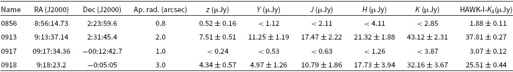
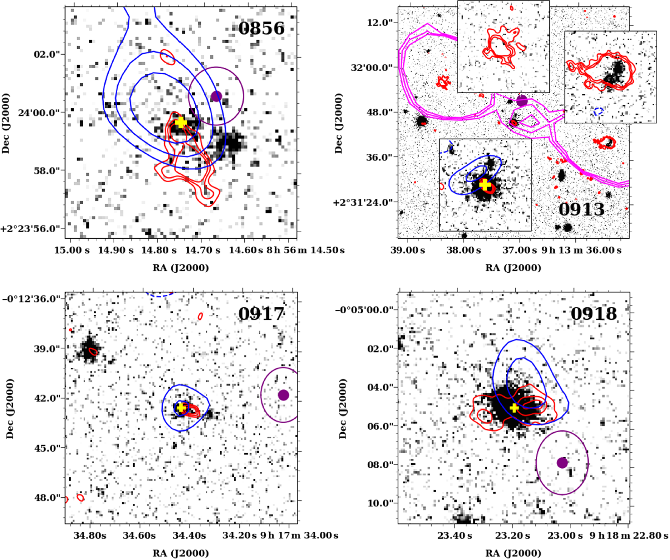
Figure 2.  $K_s$-band gray-scale VLT/HAWK-I images of our four GLEAM-selected targets with the continuum and line ALMA data overlaid as red and blue contours, respectively. The yellow cross indicates the coordinates for the ALMA spectra presented in Figure 4, and the purple circles are the GLEAM IDR3 position with their uncertainties as ellipses. The red contours represent the ALMA continuum emission (at
  $3, 4, 5, 10, 15\sigma$ with
 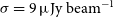 $\sigma=9\,\upmu\text{Jy beam}^{-1}$) later. The blue contours show, at lower resolution (see Section 3.3 and 4.1), the integrated detected lines in the spectra (see Figure 4) as follows (solid for positive signal, dashed for negative). 0856 (top left), the blue contours are the average-stacked CO emission at
  $2\sigma$,
  $3\sigma,$ and
  $4\sigma$ with
  $\sigma=140\,\upmu\text{Jy beam}^{-1}$. 0913 (top right), the blue contours are the detected line at 108 (at
  $-2, 2, 3\sigma$ with
  $\sigma=140\,\upmu\text{Jy beam}^{-1}$, see also Section 4.3). Note this image covers a much larger field of view (
 ${\sim} 1\,\textrm{arcmin}$) compared to other images. We overlay the 19 GHz ATCA image as magenta contours at
  $3, 4, 5\sigma$ with
  $\sigma=70\,\mu\text{Jy beam}^{-1}$. The insets show a close-up of the core and lobes. 0917 (bottom left), the blue contours are the average-stacked CO lines at
  $2, 3\sigma$ with
  $\sigma=160\,\mu\text{Jy beam}^{-1}$. 0918 (bottom right), the blue contours shows the CO line at
  $2, 3\sigma$ with
  $\sigma=160\,\mu\text{Jy beam}^{-1}$.
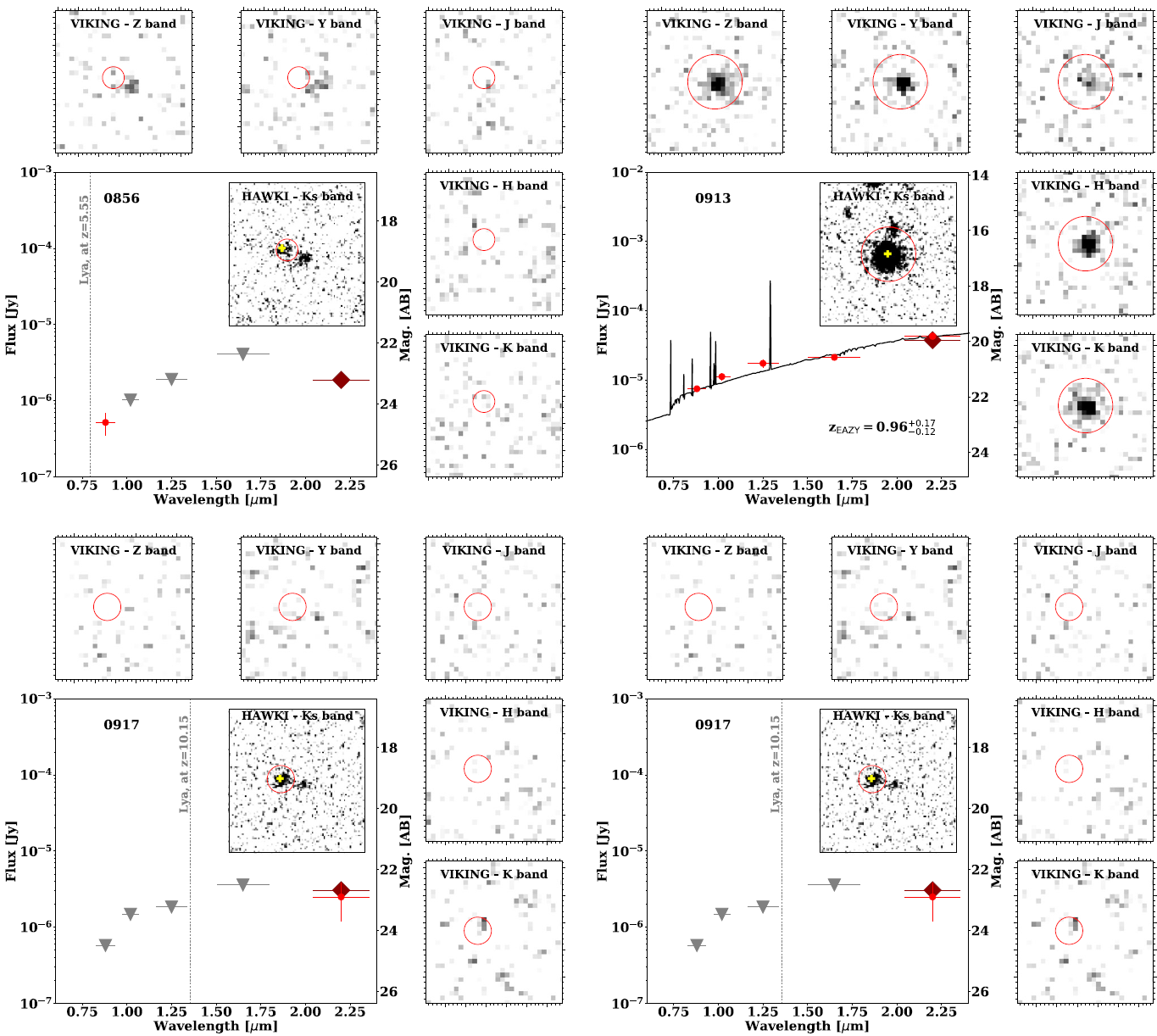
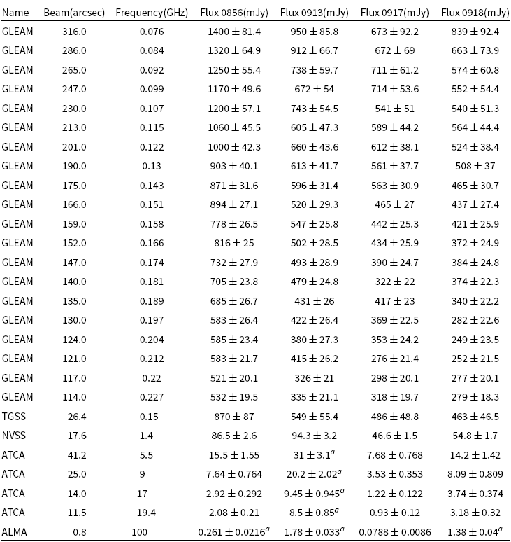
Figure 3. The NIR SEDs for our four sources with insets presenting each of the corresponding NIR images. We report the flux density (or  $3\,\sigma$ upper limit) for each band in Table 3. The circles in the insets are the apertures defined from the HAWK-I images (close insert) and also applied to the VIKING images (outer inserts). The dark large diamonds are the HAWK-I measurements. The grey symbols report the VIKING
  $3\sigma$-sensitivity in the case of non-detections. The horizontal error bars are the FWHM of the bands (zY JHK). The yellow crosses indicate the coordinates for the extraction of the ALMA spectra presented in Figure 4. For the two sources with potential confirmed redshifts (0856 and 0917), we indicate the observed wavelength of the Lyman-
 $\alpha$ line. For the two other sources (0913 and 0918), we present the best fit model for photometric redshift determination performed with eazy (see Section 4.2.2).
3.2. ATCA follow-up observations
To fill the spectral gap between 1.4 GHz and the ALMA observations at 100 GHz, we followed up the sources with the ATCA (Frater, Brooks, & Whiteoak Reference Frater, Brooks and Whiteoak1992) over a 5 h period on 2018 December 2 under the project code CX420. Using the Compact Array Broadband Backend (Wilson et al. Reference Wilson2011), 2.048 GHz bandwidth observations were conducted at nominal central frequencies of 5.5, 9.0, 17.0, and 19.0 GHz in the compact H168 array configuration. For the 5.5 and 9.0 GHz observations, we used PKS 1934-638 to establish an absolute flux density consistent with the Baars et al. (Reference Baars, Genzel, Pauliny-Toth and Witzel1977) standard (Partridge et al. Reference Partridge, López-Caniego, Perley, Stevens, Butler, Rocha, Walter and Zacchei2016) as well as to derive our bandpass correction. For the 17.0 and 19.0 GHz data, we used PKS B0420-014 to produce our bandpass correction. Across all observing frequencies, we targeted 0906+015 for phase calibration at least once every 10 min.
The data were calibrated and imaged using the miriad software package (Sault, Teuben, & Wright Reference Sault, Teuben and Wright1995) following standard procedures. They were loaded into miriad using atlod and flagged for RFI using the guided automated flagging pgflag task. During this stage, it was revealed that much of the 19.0 GHz data suffered from a broadband RFI, likely from a nearby satellite. As a consequence about 1 000 channels were flagged near the centre of the band. Next an initial bandpass and flux scale were established for the 5.5 and 9.0 GHz data with mfcal and gpcal using the calibrator PKS 1934-638 as a reference spectrum. These solutions were then gpcopyed over to the 0906+015 and time-varying phase solution was estimated using gpcal. Finally, mfboot was used to correct for any percentage-level flux scaling mismatch, and these solutions were used for the four sources. A similar procedure was used when calibrating the 17.0 and 19 GHz data, except mfcal used PKS B0420-014 to produce bandpass corrections. These were subsequently copied over to PKS 1934-638 and steps following the procedure outlined above were carried out. To allow any frequency dependent terms to be accounted for, nfbin was set to two for all appropriate calibration tasks.
Images were created using invert with a Briggs robust parameter of 2 (equivalent to a natural weighting). We did not include the 6th ATCA antenna, separated by  $\sim4.5\,\text{km}$ from the central core of the H168 array. Owing to the large fractional bandwidth of the data, the wideband imaging deconvolution task mfclean (Sault & Wieringa Reference Sault and Wieringa1994) was used. Next, restor and linmos were used together to deconvolve telescope artefacts and apply primary beam corrections while accounting for the spectral index terms constrained by mfclean for each of the clean components. The final sensitivity on the images reaches typically the
 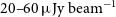 $20\text{--}60\,\upmu\text{Jy beam}^{-1}$ level and the final synthesised beam goes from
  $48\,\textrm{arcsec}\times 34\,\textrm{arcsec}$ to
  $13\,\textrm{arcsec}\times 9\,\textrm{arcsec}$ from 5.5 to 19 GHz, respectively. Finally, we ran aegean (Hancock, Trott, & Hurley-Walker Reference Hancock, Trott and Hurley-Walker2018) on each image to extract the flux observed in the continuum images and report the total flux densities in Table 4.
Table 4. Radio flux density summary for our four radio galaxies. The reported GLEAM values below are from the public release, not IDR3.
a The flux densities are the sum of multiple components.
3.3. ALMA Band 3 follow-up observations
As our four sources were close together in G09, we could optimise our observing strategy by sharing overheads. Our main goal is to detect one or more CO lines in order to determine a secure redshift. At  $z>5$, we expect two or more lines in the full frequency range. Our project 2017.1.00719.S was observed on 2018 January 25 and 26 in configuration C43-5 (total
  $\sim6\,\text{h}$) and with a high perceptible water vapour (PWV) of 5.2 and 6.5 mm, respectively. We requested a spectral scan in Band 3, covering the 84–115 GHz range with five different tunings. All processing is performed with casa in version 5.3.0 (McMullin et al. Reference McMullin, Waters, Schiebel, Young and Golap2007). We inspect the visibilities to check for extra-flagging with the plotmscasa routine, merge the five sub-cubes at different frequencies (tunings) into a single cube per source.
3.3.1. Continuum image and flux extraction
We created a 30 GHz-continuum (total ALMA bandwidth) centred at  $\nu_{\rm sky}=100\,\text{GHz}$ image using natural weighting in order to maximise sensitivity for each source. The final images present an averaged synthesised beam of
  $0.7\,\textrm{arcsec}\times0.8\,\textrm{arcsec}$, a noise of about
  $9\,\upmu\text{Jy beam}^{-1}$, and are presented as red contours in Figure 2. We ran Aegean with all default parameters to derive the photometry and report the results in Table 4.
3.3.2. Spectral cubes, spectrum extraction, and line detection
As the expected line strength was low and the atmospheric conditions non-optimal (high PWV, see Section 3.3), we decided to taper our data by a 3 arcsec Gaussian beam in order to minimise the noise contribution of the longest baselines (our longest baselines are 1.4 km) in order to increase our signal to noise for detection. We also smoothed the data in frequency space from 20 to 80 MHz channels. The corresponding final sensitivity in the inverted cubes is 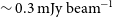 $\sim0.3\,\text{mJy beam}^{-1}$ for 80 MHz-width channels.
The  $K_s$-band imaging was key to finding the host galaxies, and we therefore extracted spectra over
  $0.8\,\textrm{arcsec}$ radius centred on the
  $K_s$ positions. From this, we subtracted a background spectrum created from a sky annulus (radius of
  $3.5$–
 $5.5\,\textrm{arcsec}$). We present the spectra in Figure 4. We then ran a 1D line-finder (sslfFootnote b) with a low threshold for line detection (
 $\text{f}_{\rm thres}>3\sigma$ and line width larger than four channels). The only exception is 0917, where we used a lower threshold (
 $\text{f}_{\rm thres}>2.5\sigma$, see Section 4.3). We found weak emission lines in these spectra, and we verified they were also successfully detected in higher resolution spectra with 20, 35, 40, 60, and 75 MHz channel-width. We describe the method for the redshift determination in Section 4.3.
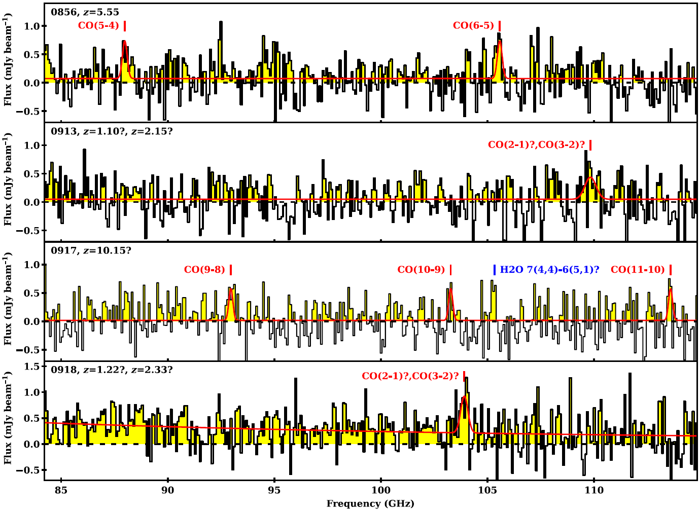
Figure 4. The ALMA spectra with an 80 MHz resolution for our four sources extracted from the positions of the hosts as seen in the  $K_s$-band images. Table 5 reports the line flux densities. We also present the fitting of a simple model for the observed lines. In the case of a possible redshift solution, we indicate the corresponding line transitions. See Section 4.3 for more details on the fitting and the redshift determination.
4. Results
Due to the complex nature of our sources and our multi-wavelength dataset, we will present our results in the following order. First, we will review individual morphology from our continuum emission (Figure 2). Second, we will present the spectral information through their SEDs. Third, we will determine the redshifts of our sources from their ALMA spectra and previously introduced information, and finally, we explore their NIR and radio properties.
4.1. Multi-wavelength morphologies
GLEAM 0856: The  $K_s$-band image reveals two sources. The resolved ALMA continuum (red contours) consists of an extended component (with a
  $>5\sigma$ peak) over 2–3 arcsec. Two very faint extensions eastward and southward are also detected at the
  $3\sigma$-level. The ALMA emission is associated with the eastern
  $K_s$-band source. We therefore consider this source to be the host of the radio galaxy and extract our ALMA spectrum from this position. This interpretation is supported by weak radio emission (
 $2\sigma$) 2 arcsec north of the host galaxy and opposite the extended radio component. The stacked CO emission covers the host galaxy but extends in the direction of the weak northern radio emission.
GLEAM 0913: This radio source is the most extended of our sample in the radio (see Figure 2). The ALMA continuum image presents three components with a total separation of  $\sim+35\,\textrm{arcsec}$. These components appear to be related as the 19 GHz ATCA morphology (magenta contours) is consistent with a lobe-core-lobe morphology.
The identification of the host galaxy is straightforward as the central radio component is co-located with a bright source in the  $K_s$ band (see the inset of Figure 2). The corresponding NIR source is actually detected in the VIKING images but was offset
  $\sim 6\,\textrm{arcsec}$ to the north of our low-frequency centroid radio position (see purple circle in Figure 2). This demonstrates that higher resolution continuum data are essential to identify the host galaxy. We also show the moment 0 map of the ALMA spectral line at 109.89 GHz as blue contours in the insets.
GLEAM 0917: This source is the faintest of our sample in both NIR and radio. We see a faint continuum at 100 GHz, detected at the 5 $\sigma$-level. We also see two faint sources in the
  $K_s$ image with the eastern one associated with the ALMA continuum detection which we identify as the host galaxy. The ALMA spectrum shows four weak lines, which we discuss in more detail in Section 4.3. We present the average-stacked lines as the blue contours and see a detection centred on our object.
GLEAM 0918: The  $K_s$ image shows a bright source co-located with a double source in the ALMA continuum, likely corresponding to two synchrotron lobes. This host galaxy also has a detection in the VIKING data but was misidentified due to the low-resolution radio data (note the large offset of 6 arcsec of the GLEAM position from this
  $K_s$ source). The higher resolution ALMA data have allowed us to unambiguously identify this source with the VIKING counterpart. Only one line is detected in the ALMA spectra, indicating likely a lower redshift source (as suggested by the strong VIKING detection).
4.2. Radio and optical SEDs
4.2.1. Radio broadband SEDs
The complete radio SED from 76 MHz to 100 GHz for each source is presented in Figure 5 and Table 4. Note that an absolute calibration uncertainty is added in quadrature to each data-point uncertainty. We assume 8% for GLEAM (Hurley-Walker et al. Reference Hurley-Walker2017), 3% for NVSS (Condon et al. Reference Condon, Cotton, Greisen, Yin, Perley, Taylor and Broderick1998), and 10% for ALMA.
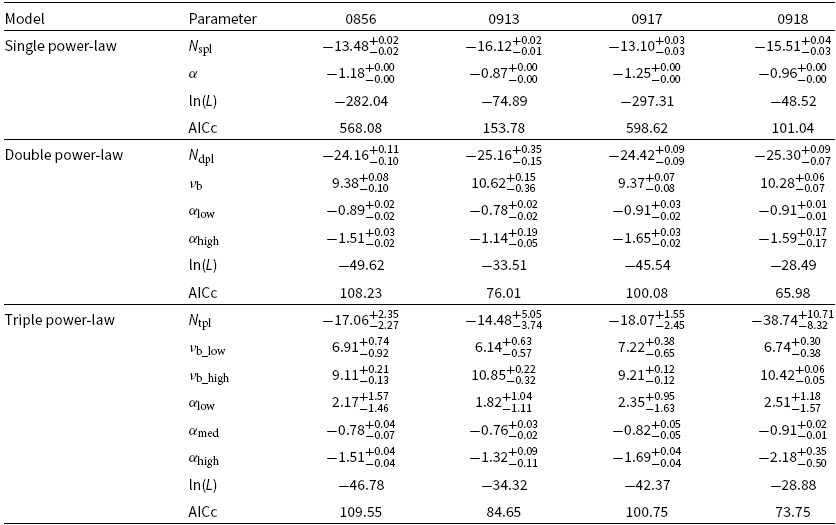
We perform SED fitting in order to characterise the break frequencies and change of spectral indices across the four decades in frequency for the total integrated emission. We use the SED fitting code MrMoose (Drouart & Falkendal Reference Drouart and Falkendal2018), using three different models to fit the data: a simple power-law, a double power-law with a break frequency, and a triple power-law with a double break frequency. We define the functions as followsFootnote c:
 \begin{eqnarray}S_\nu^{\rm spl}&=&N_{\rm spl}(\nu_{\rm obs})^{\alpha}, \end{eqnarray}
 \begin{eqnarray}S_\nu^{\rm dpl}&=&N_{\rm dpl}(\nu_{\rm obs})^{\alpha_{\rm low}}\left(\frac{\nu_{\rm obs}}{\nu_{\rm b}}\right)^{\alpha_{\rm low}-\alpha_{\rm high}}, \end{eqnarray}
 \begin{eqnarray}S_\nu^{\rm tpl}&=&N_{\rm tpl}(\nu_{\rm obs})^{\alpha_{\rm low}} \nonumber \\[3pt] & & \times\left[1+\left(\frac{\nu_{\rm obs}}{\nu_{\rm b\_ low}}\right)^{|\alpha_{\rm low}-\alpha_{\rm med}|}\right]^{\rm sgn(\alpha_{\rm med}-\alpha_{low})}\nonumber \\[3pt]& & \times\left[1+\left(\frac{\nu_{\rm obs}}{\nu_{\rm b\_high}}\right)^{|\alpha_{\rm med}-\alpha_{\rm high}|}\right]^{\rm sgn(\alpha_{\rm high}-\alpha_{\rm med})}\end{eqnarray}
where  $\nu_{\rm obs}$ is the observed frequency,
  $\nu_{\rm b}$,
  $\nu_{\rm b\_low}$, and
  $\nu_{\rm b\_high}$ the break frequencies,
  $\alpha$,
  $\alpha_{\rm low}$,
  $\alpha_{\rm med}$, and
  $\alpha_{\rm high}$ the spectral indexes, and sgn referring to the sign of the operation. Note the absolute value for the spectral index difference.
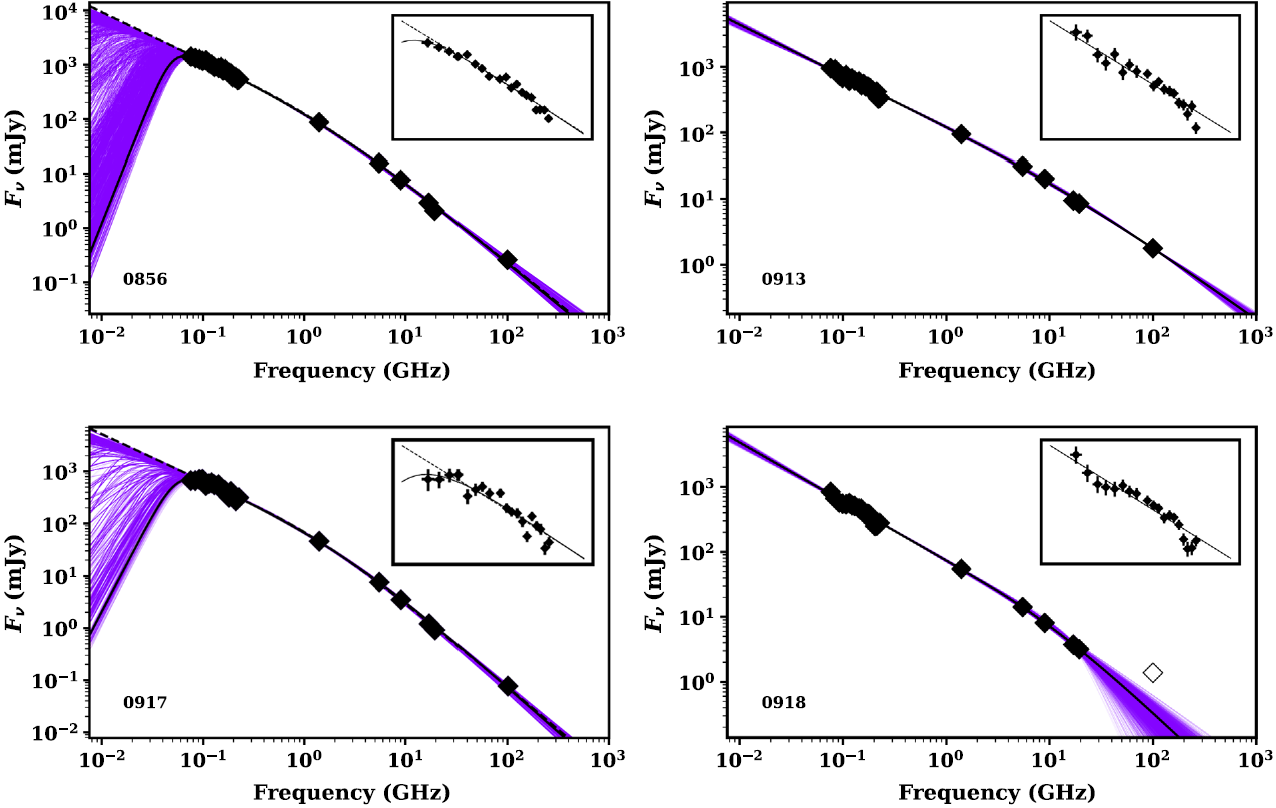
Figure 5. The observed-frame radio SED for each source fitted with the triple power-law model for 0856 and 0917 and the double power-law model for 0913 and 0918 (all plotted as solid black lines). Uncertainties are plotted, but are hidden by the symbols. The uncertainty is represented by the scatter in the purple lines (see Section 4.2.1). For 0856 and 0917, we also present the best fit for the double power-law as a black-dashed line. The data in each SED, with number of data points in parentheses, comprise, from low to high frequency, MWA (20), TGSS (1), NVSS (1), ATCA (4), and ALMA (1). Note the open diamond for the ALMA data for 0918 is not included in our fit (see Section 4.2.1). Note that uncertainties are plotted, but are smaller than the symbol size. The insets are a zoom on the MWA data with the best fit(s) from the wider SED overlaid.
We are interested here in the SED from the total flux emission (sum of all components, see Table 4), and therefore only focus on models with differing numbers of power-laws. Characterising the physical processes at work further is beyond the scope of this paper, especially given that only one source has a definite redshift (see Section 4.3). We compare the relative likelihood for each model with the Akaike Information Criteria (AICc; Akaike Reference Akaike1974; Burnham & Anderson Reference Burnham and Anderson2002) which is defined as:
 \begin{equation}{\rm AICc} = 2k-2{\rm ln}(L) + \frac{2k(k+1)}{(n-k-1)},\end{equation}
where n the number of data points, k the number of free parameters, and ln(L) the maximum of the likelihood function (calculated with MrMoose). Note the first term, 2k, penalising the addition of free parameter and the last term an added correction in the case of small sample sizes (this can be seen as an extra penalty for an increased number of free parameters on small samples). We report the results of the fitting in Table 6 and plot the preferred model in Figure 5.
The AICc criteria indicate that the model which best represents the sources overall is the double power-law model. Moreover, it is clear that the triple power-law, while providing a good fit, does not improve significantly the AICc for 0918 and 0913 even with the curvature in the MWA frequency bands. As for 0856 and 0917, the AICc scores are similar for the double and triple power-law models which indicate that both models are equally preferred. We note that the best fit for the triple power-law reproduces the curvature in the MWA data, albeit with a large uncertainty on the spectral slope at lower frequency,  $\nu<70\,\text{MHz}$, where the fit is unconstrained. For all sources, we measure a double power-law break frequency in the 2–42 GHz range (note how the ATCA data provide for a strong constraint here). The lower frequency spectral index is moderately steep with
  $\alpha<-0.7$ and in reasonable agreement with the GLEAM-only spectral index from our polynomial fit used in Section 2. The higher frequency spectral index is systematically steeper by
  $\Delta(\alpha)=0.36-0.7$.
In the case of 0918, the ALMA continuum point is not included in the model fitting as it would imply an up-turn/flattening of the radio SED or a separate component. This could be due to either a separate synchrotron component with a very high-frequency turn-over or possible inverse Compton emission from the lobes. Without further data, it is impossible to model either possibility.
Table 5. ALMA spectra line measurements: detected and fitted. The detections have a central frequency, peak flux, and width all with uncertainties. The fitted measurements are too all detected lines simultaneously and give a background continuum, amplitude, width, and redshift (all with uncertainties).
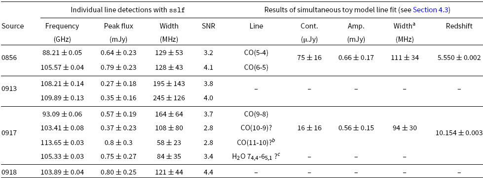
aThe line width here corresponds to 930 ± 120 km s−1 and 750 ± 200 km s−1 when converted into the rest-frame for 0856 and 0917, respectively. bThis line is only detected at very marginal level, note the width being lower than the spectral resolution (80 MHz).cThis line is not fitted simultaneously with the CO lines.
4.2.2. Broadband optical-NIR SEDs
We note that two sources (GLEAM 0913 and 0918) are detected in all VIKING NIR bands due to misidentification arising from the low-frequency, low-resolution radio data (see Section 4.1). Having access to a significant part of the SED, we use the photometric redshift code eazy with default settings (Brammer et al. Reference Brammer, van Dokkum and Coppi2008) to estimate the redshift of these two sources. While presenting large uncertainties, these redshifts are useful when compared with the ALMA spectral line redshift solutions (see next sub-section). We obtain  $z_{\rm 0913}=0.96^{+0.17}_{-0.12}$ and
  $z_{\rm 0918}=0.77^{+0.22}_{-0.26}$ with 68% confidence limits. Of the two other sources, 0856 is weakly detected in z-band and 0917 is not detected in any VIKING band. We can obtain some information on the galaxy host using the K–z relation (see Figure 7 and Section 4.4.1).
4.3. Redshift determination from the ALMA spectra
Given the spectral scan in Band 3 (84–115 GHz), we have three possibilities:
No line is detected in this range and we are either observing a source located at a redshift with no CO line in this range (at
$0.36<z<1.0$ and $1.74<z<2.0$) or a source with molecular lines too faint to be detected,A single line is detected and the redshift solution is ambiguous but constraints may be derived from the absence of other molecular lines, or
Two lines or more are detected across the spectra and the redshift can be unambiguously measured and/or any interloper can be clearly identified.


This is the method used by the SPT team to determine the redshifts of strongly lensed sub-mm galaxies (Weiß et al. Reference Weiß2013; Strandet et al. Reference Strandet2016). Note that while working extraordinary well on lensed sources, thanks to their compactness and magnification, using this technique on un-lensed sources is far more challenging. We designed our sample selection to find multiple lines (if at  $z>3.0$), that is, falling into option (iii) above and therefore obtaining an unambiguous redshift measure.
We examine our lines sequentially in decreasing signal-to-noise order, assuming that we are observing a CO line and therefore predict the frequency of other molecular lines, CO, [CI], and  $\text{H}_2\text{O}$ (using splatalogueFootnote c) for the corresponding redshifts (the vertical bars in Figure 6). We do not consider the HCN and HCO+ lines as they are expected to be much fainter. With even a single line identification, we can exclude certain redshift solutions given that other lines should be detected in our broad frequency range. In the case of multiple line detection, we compare the estimated frequencies with the other detected lines with sslf. Our approach is summarised in Figure 6, where a good match is usually obvious (e.g. 0856). Thus, we perform a fitting on the spectra using this redshift prior, adding the corresponding number of Gaussians required to reproduce the spectra (note that we assume the exact same amplitude and width for all lines). We also add a continuum component as a constant across the frequency range (excepted 0918 where a spectral index is added as a strong gradient is observed in the spectra, see Figure 4 and Table 5). We now review our sources individually, by increasing the order of complexity.
Table 6. Results from the observed-frame radio SED fitting. We report the best fit parameter for each model (single, double, and triple power-law from top to bottom) along with their uncertainties defined as the 25 and 75 percentiles. The break frequencies are given as the log of the frequency in Hz, ln(L) refers to the log of the maximum of the likelihood function used to calculate the AICc criteria (see Equation 5).
GLEAM 0918: A single detected line is centred at 103.89 GHz which would translate to 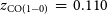 $z_{\rm CO(1-0)} \,=\,0.110$,
 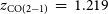 $z_{\rm CO(2-1)} \,=\,1.219$,
 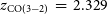 $z_{\rm CO(3-2)} \,=\,2.329$,
 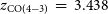 $z_{\rm CO(4-3)} \,=\,3.438$, and
 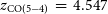 $z_{\rm CO(5-4)} \,=\,4.547$ (see Figure 6). We can discard the
  $z=3.438$ and
  $z=4.547$ solutions as the [CI](1-0) should appear in our frequency range. Conversely, we also can discard the lowest redshift solution (
 $z=0.110$) as the related radio luminosity (see Figure 8),
  $K_s$ luminosity (see Figure 7), and the predicted CO flux (see Figure 9) are not compatible for such a low-redshift source. Hence, this source is at
  $z=1.219$ or
  $z=2.329$. Given the result of the photometric redshift (see Section 4.2.2), the first solution appears the more likely.
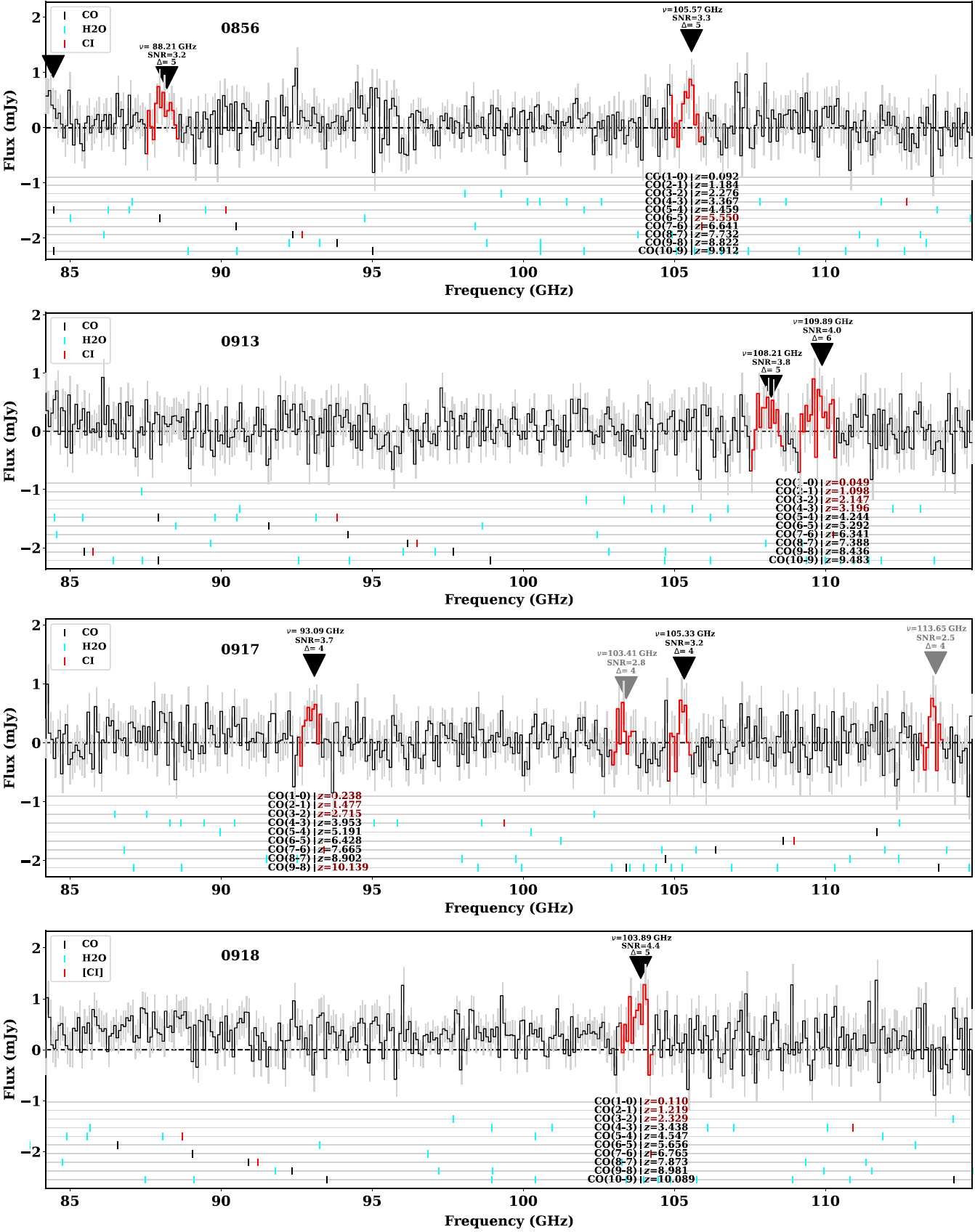
Figure 6. Redshift determination for our four sources from the ALMA spectra. This figure shows the 1D spectra extracted at the position indicated in Figure 2 and presented in Figure 4. The grey error bars are showing the rms per channel. The downward triangles and the red part of the spectra refer to the detection of the lines by sslf (see Section 3.3). The line characteristics are reported above the markers (central frequency, signal-to-noise ratio, and FWHM in number of channels). We highlighted the detections in the 2.5-3 $\sigma$ range in grey for 0917. Taking the highest signal-to-noise line and assuming this is a CO line, the vertical black markers are reporting the combination of the possible redshift along with the prediction of the other transition CO lines, as well as [CI] and
  $\text{H}_2\text{O}$. We highlight the potential redshift solutions in dark red (see section 4.3).
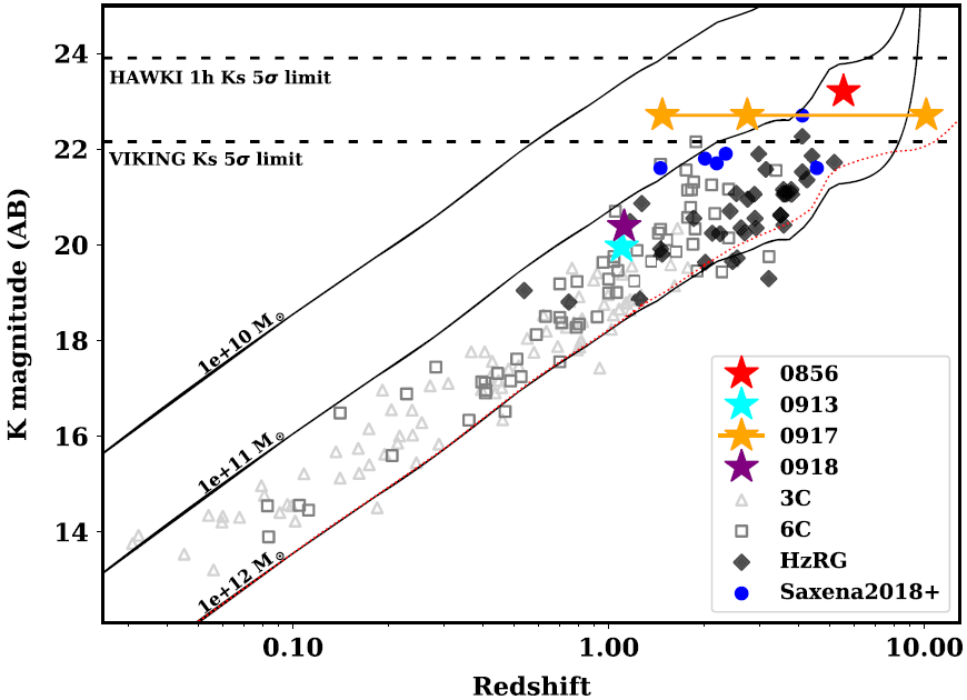
Figure 7. K–z relation diagram showing the observed K–band magnitude against the redshift of known powerful radio galaxies (see legend). Our four candidates are represented with coloured stars and with lines connecting possible redshift solutions from a combined analysis of all the data in hand. The VIKING and HAWK-I detection limits are indicated by dotted lines. The tracks correspond to the elliptical templates from PÉGASE.2 (Fioc & Rocca-Volmerange Reference Fioc and Rocca-Volmerange1997) scaled to reported stellar masses.
Figure 8. Radio luminosity at rest-frame 500 MHz (top) and 3 GHz (bottom) plotted against redshift of samples of powerful high-redshift radio galaxies. We present our four objects as stars with a line connecting multiple redshift solutions. The solid lines are luminosities determined from the SED within our frequency coverage and the dashed line is where an extrapolation is required from our best SED fitting (below the GLEAM limit, at  $<$70 MHz). We also plot the sample from Saxena et al. (Reference Saxena2019), and the quasar from Bañados et al. (Reference Bañados, Carilli, Walter, Momjian, Decarli, Farina, Mazzucchelli and Venemans2018b), recalculated at the relevant frequency from the flux densities and spectral indexes provided.
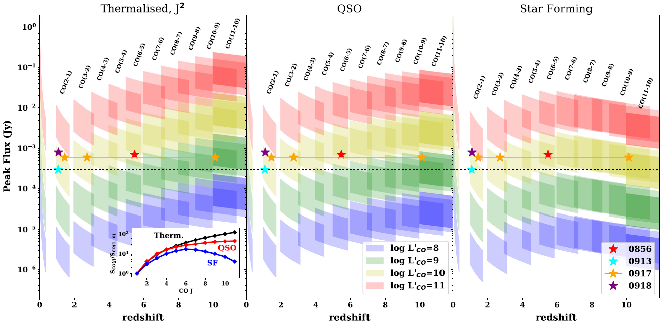
Figure 9. Prediction of CO peak flux density for transitions within ALMA Band 3 depending on (i) the CO SLED (panels left to right), (ii) the intrinsic CO brightness (middle insert) and the width of the line (shaded area), and (iii) the redshift (the x-axis). The stars corresponding to our four sources per the lower right legend. For sources with more than one possible redshift a line connects them. The CO SLEDs (presented in the inset in the lower left) follow a thermalised case ( $\text{J}^2$, left), a typical quasar (centre), and typical star-forming galaxies (right), taken from Carilli & Walter (Reference Carilli and Walter2013).
GLEAM 0913: The two lines detected in 0913 are too close to each other to come from two different CO transitions (and too far apart to have originated from the same source). Overlaying the contours of the two lines on the  $K_s$-band image shows that the 108.21 GHz line is very likely spurious. We therefore do not consider this line anymore. From the 109.89 GHz line, the redshift solutions are
  $z_{\rm CO(1-0)}$ = 0.049,
  $z_{\rm CO(2-1)}$ = 1.098,
  $z_{\rm CO(3-2)}=2.147$, and
  $z_{\rm CO(4-3)}$ = 3.196. Any higher in redshift and we would see a second line in our frequency coverage (either [CI] or a CO transition, see Figure 6). For the same reason as for 0918, we can discard the lowest redshift solution. When comparing these redshift solutions with the phot-z estimate (Figure 3), the solution at
  $z=1.098$ appears most probable. Additionally, no radio source of this size has been observed above
  $z\sim 2.5$ (De Breuck et al. Reference De Breuck2010).
GLEAM 0856: This source is the prototype source that our selection method is designed to find. Two lines are detected at 88.21 and 105.57 GHz. Assuming they are both CO, the redshift is unambiguously determined from the fit as  $z=5.550\pm0.002$ (Table 5).
4.3.1. The complex case of GLEAM 0917
GLEAM 0917 is the most complex spectrum to interpret. If considering only the two lines detected above 3 $\sigma$ at 93.08 and 105.33 GHz, these detections do not provide any redshift solution for a single source (see Figure 6). Alone, the 93.08 GHz line would correspond to
  $z_{\rm CO(2-1)}=1.477$ and
  $z_{\rm CO(3-2)}=2.745$ (we discard the lower redshift CO(1-0) solution as for 0918). However, while not impossible, these redshift solutions present some problems with our NIR SED. The
  $K_s$ magnitude would point to a fainter system. Considering the 105.33 GHz line on its own gives the solutions of
 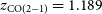 $z_{\rm CO(2-1)}=1.189$ and
 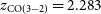 $z_{\rm CO(3-2)}=2.283$. By decreasing the line detection threshold of sslf to 2.5
 $\sigma$, two other lines are detected at 103.41 and 113.65 GHz (indicated by grey triangles in Figure 6). The addition of these two lines along with the 93.08 GHz line does provide a unique redshift solution at
  $z=10.154\pm0.003$ for CO(9-8), CO(10-9), and CO(11-10). However, this possibility comes with various caveats.
Firstly, the width of the lines is not similar; they become narrower with increasing frequency. In particular, the highest frequency line is best fit with a width on par with the one tapered  $80\,\text{MHz}$ bin. We therefore applied the same procedure to our smaller channel-width cubes. The three lines are still detected and still become narrower with increasing frequency. Part of this effect could originate from the noise increase due to the increasing atmospheric opacity (relatively strong towards the end of the band at
  $\nu>110\,\text{GHz}$ in bad weather conditions).
Secondly, to exclude the possibility that these lines are spurious, we generated simulated spectra with the same Gaussian noise rms, but no true signal, and run sslf with the exact same parameters ( $f_{\rm thres}=2.5\sigma$ and line width larger than four channels). Assuming a conservative frequency difference between the central frequency of the different CO transition lines to be a shift of
  $<3$ channel bins with respect to each other (corresponding to a significant shift up to 240 MHz), out of
  $10^6$ simulated spectra only 626 cases (corresponding to a 0.06% chance) are able to reproduce a spectra with three detected ‘lines’ at
  $>2.5\sigma$. Note that this matching makes an assumption neither on the line width (except being larger than four channels to be detected by sslf) nor on the amplitude of the lines. Any further constraints on these parameters will result in an even lower probability. We also note that all physical quantities (described in the following sections), the
  $K_s$ magnitude (Figure 7), the 500 MHz and 3 GHz luminosities (Figure 8), and the CO properties (Figure 9) are consistent with a powerful radio-loud AGN at such an extreme redshift.
Thirdly, the  $z=$10.15 solution would suggest that we are possibly observing a water line at 105.33 GHz. The emission of
  $\text{H}_2\text{O}$ is known to be rather complex to trace given the numerous excitation states available (Werf et al. Reference Werf2011). This line is nonetheless routinely detected at high redshift (Weiß et al. Reference Weiß2013; Wang et al. Reference Wang2013; Gullberg et al. Reference Gullberg2016). Wilson et al. (Reference Wilson2017) combined the sub-mm spectra of a large number of star-forming sources in the
  $0.1<z<4$ range. The closest in frequency for this given redshift is the
  $\text{H}_2\text{O}$
 $7_{4,4}-6_{5,1}$ transition (
 $\nu_{\rm rest}=1172.526\,\text{GHz}$) and is blue-shifted compared to the systemic redshift by
  $\sim300\,\text{km\,s}^{-1}$. However, this line has not been detected at any redshift so far and the condition required to emit such a line would mean we would observe other lines in the full frequency range. The closest observed waterline transition is the
  $\text{H}_2\text{O}$
 $3_{2,1}-3_{1,2}$ (at
  $\nu_{\rm rest}=1162.911\,\text{GHz}$ detected by Wilson et al. Reference Wilson2017). However, this corresponds to a
  $\sim 2500\,\text{km\,s}^{-1}$ blueshift, which appears to be very unlikely. We therefore conclude that this line might be from a different object along the line-of-sight, or perhaps more likely, a spurious detection.
4.4. Interpretation
4.4.1. NIR observations and the K– z relation
The  $K_s$ magnitudes provide us with our first insight of the properties of the sources, as well as helping to solve the case of degenerate redshift solutions as presented in Section 4.3. Figure 7 shows our sources along with samples of powerful radio galaxies samples (3C, 6C, and other HzRGs; Lilly & Longair Reference Lilly and Longair1984; Eales et al. Reference Eales, Rawlings, Law-Green, Cotter and Lacy1997; van Breugel et al. Reference van Breugel, Stanford, Spinrad, Stern and Graham1998). The K–z relation shows that powerful radio galaxies form a correlation in observed K-band and redshift space which is modelled as being due to emission from massive galaxies (
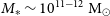 $M_*\sim 10^{11-12}\,{\rm M}_{\odot}$, Rocca-Volmerange et al. Reference Rocca-Volmerange, Le Borgne, De Breuck, Fioc and Moy2004). The classic interpretation of this result is that the most luminous radio galaxies are powered by the most massive black holes lying in the most massive galaxies. Evidence for the large black hole masses comes from Nesvadba et al. (Reference Nesvadba, Lehnert, De Breuck, Gilbert and van Breugel2008) and Drouart et al. (Reference Drouart2014). Hence, from this diagram, and as mentioned previously (Section 4.3), the most likely redshift solutions for 0913 and 0918 appear to be consistent with the main relation. The K–z relation arguably becomes less certain at the redshifts we aim to probe here (
 $z>5$) as the observed K-band shifts from the blue optical to the ultra-violet rest-frame. At these wavelengths, the star-formation properties (star formation rate, age of the stellar population, and dust content) can account for significant differences to the emission. We see that the redshift solutions for 0917 are offset from the main relation. However, no powerful radio galaxy has been detected with
  $K\le 21.5$ at
  $z>5$.
4.4.2. Radio luminosity interpretation
Having access to the radio SED from 70 MHz to 115 GHz, one can determine the rest-frame 500 MHz and 3 GHz luminosities. We show the distribution of these luminosities with redshift in Figure 8 from the SEDs previously shown in Figure 5. Note that the lowest frequency GLEAM data point (70 MHz) allows us to determine the 500 MHz luminosity from data only up to  $z=6.14$. After that we must extrapolate (via our best fit SED in our case) to estimate luminosities at higher redshift. The 3 GHz rest-frame luminosity is not affected by this observational limit.
Figure 8 shows 0913 and 0918 have comparable radio luminosities to the bulk of previous samples of high-z powerful radio galaxies. In the case of 0856, the source also appears very similar to the HeRGÉ sample (De Breuck et al. Reference De Breuck2010) but at higher redshift. For 0917, the luminosity at  $z=10.15$ would be consistent with a very bright source, but nothing abnormally bright when compared with a similar sample at lower redshift. We also note that the break frequency for the four objects differs significantly for the double power-law model. The higher redshift objects (GLEAM 0856 and potentially GLEAM 0917) have lower frequency breaks, consistent with them lying at higher redshift.
4.4.3. Molecular gas properties and predictions
With a measurement of the CO flux, we can explore the properties of the molecular gas. In Figure 9, by assuming a spectral line energy distribution (SLED, the three panels, see insets) and an intrinsic  ${\text{L}^\prime_{\rm CO}}$, we can predict the integrated flux in each of the CO lines as a function of redshift (shaded coloured areas). For each CO transition line, the horizontal span shows the frequency range of the given CO transition accessible with the ALMA Band 3 (84–115 GHz), and the vertical span shows the line width range (limited here to 200–
 $1000\,\text{km\,s}^{-1}$). Note how the negative k-correction—very similar to that observed at sub-mm wavelength (see Blain et al. Reference Blain, Smail, Ivison and Kneib1999)—allows for a relatively constant detection limit with increasing redshift.
We also report our rms sensitivity (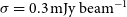 $\sigma=0.3\,\text{mJy beam}^{-1}$ per 80 MHz channel-width) as the black-dotted line. This diagram directly shows that ALMA provides us with easy access down to an intrinsic CO luminosity
  ${\text{L}^\prime_{\rm CO}}=10^{10}{\text{K km s}^{-1}\text{ pc}^{2}}$, relatively independently of the redshift of the source. The final sensitivity is mainly driven by the shape of the SLED and, therefore, the excitation conditions of the source are the dominating factor, especially at the higher redshift end, the stronger the excitation properties, the lower in intrinsic luminosity we can reach. For a given source, the discrimination between the excitation mechanisms will require observations of other CO transitions. One interesting point to note is independently of the intrinsic CO SLED, 0856 seems to lie around
  ${\text{L}^\prime_{\rm CO}}\,=\,10^{10}{\text{K km s}^{-1}\text{ pc}^{2}}$. For 0856 at
  $z=5.55$, we can estimate a
  ${\text{L}^\prime_{\rm CO}}\,=\,4\times10^{10}{\text{K km s}^{-1}\text{ pc}^{2}}$. This value—as well as the line width (
 $930\,\text{km s}^{-1}$) —is very similar to other radio galaxies and quasars at lower and similar redshift (Carilli & Walter Reference Carilli and Walter2013, see their Figure 5).
5. Discussion
5.1. Selection efficiency
Out of four sources observed with ALMA, one can be considered as a bona fide detection of a powerful radio galaxy at  $z=5.55$. For our definition of powerful radio galaxies (
 $L_{\rm 500\,MHz}>10^{27}\,\text{WHz}^{-1}$), with 0856 we have already demonstrated the capability to break the 20-yr-old record from van Breugel et al. (Reference van Breugel, De Breuck, Stanford, Stern, Röttgering and Miley1999).
Moreover, we have a very tentative candidate at  $z=10.15$. We stress that this candidate still requires further observations to be securely confirmed. The two other sources are very likely lower redshift sources (
 $1<z<3$). While using some caution about low-number statistics, we argue that we have detected at least 1/4 sources at
  $z>5$ from our full pilot sample and possibly up to 2/4 (assuming that the 0917 is at least at
  $z>5$)—corresponding to a success rate of between 25 and 50%.
This result is in comparison to Saxena et al. (Reference Saxena2018a), who are probing lower flux densities at low frequency, and found 1 out of 32 sources at  $z>5$ (the aforementioned
  $5.72$ radio galaxy). We note however they found four additional radio galaxies at
  $4<z<5$ (Saxena et al. Reference Saxena2019). Our flux cut,
  $\text{F}_{\rm 151\,MHz}>0.4\,\text{Jy}$ (in comparison to only using a upper limit of
  $\text{F}_{\rm 151\,MHz}\le 0.2\,\text{Jy}$ such as the Saxena et al. Reference Saxena2018b) ensures we select targets with relatively strong continuum emission. This admittedly prevents the detection of intrinsically lower luminosity objects, but our high-flux density limit is of prime importance for the future direct measure of HI absorption at such extreme redshifts. Deeper surveys with the MWA will improve the signal to noise on our sources and make the model fitting across the MWA frequencies more secure.
5.2. Comparison to other high- z AGN samples
When comparing the NIR properties, the  $K_s$ magnitude is consistent with other samples of powerful radio galaxies (see Figure 7), and therefore we are preferentially selecting obscured, type 2 AGN. This result is expected given the selection from weak/non-detection in K-band from the VIKING data. In comparison, the sample of bright QSOs from Bañados et al. (Reference Bañados2016) is qualitatively brighter, in the H = 19–20 mag (AB) range, as expected from their selection to be type 1, unobscured AGN. Note that this QSO sample does not follow the K–z relation (Figure 7) as the AGN outshines the host at optical/NIR wavelength decreasing the observed K-band magnitude. Our selection is also biased to target massive systems: in the
 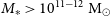 $M_*>10^{11-12}\,{\rm M}_{\odot}$ range (Rocca-Volmerange et al. Reference Rocca-Volmerange, Le Borgne, De Breuck, Fioc and Moy2004). Interestingly, the Saxena et al. (Reference Saxena2019) sample tends to select similar or somewhat less massive systems (
 $M_*=10^{10.8-11.7}{\rm M}_\odot$). Wider NIR photometric coverage is required to more accurately estimate stellar masses for our sample.
Our method is, by design, selecting the brightest radio sources in the sky (see Figure 8), unlike the recent sample described in Saxena et al. (Reference Saxena2019). This makes our sample similar in nature to previously existing samples of powerful radio galaxies (e.g. HeRGÉ, Seymour et al. Reference Seymour2007). Our two  $z>5$ radio galaxies, GLEAM 0856 and GLEAM 0917, have observed frame break frequencies around 1.4 GHz. Hence, we can compare the modelled spectral indices below this frequency to that of the Saxena sample. We find that our radio galaxies have less steep spectra than Saxena, with
  $\alpha_{\rm low}\sim -0.9$ compared to
  $\alpha_{1.4\,{\rm GHz}}^{151\,{\rm MHz}}<-1.4$. However, at higher frequencies, our radio sources have
  $\alpha_{\rm high} \sim -1.6$ which meet the Saxena selection criteria. Hence, our selection appears to favour radio galaxies with a higher rest-frame break frequency than USS selected radio galaxies and therefore potentially younger radio sources (e.g. Turner, Shabala, & Krause Reference Turner, Shabala and Krause2018).
Interestingly, out of the hundreds of optically bright AGN from the Bañados et al. (Reference Bañados2016) sample, a single one (PSO J352.4034-15.3373 at  $z=5.84\pm0.02$ Bañados et al. Reference Bañados, Carilli, Walter, Momjian, Decarli, Farina, Mazzucchelli and Venemans2018b) is detected with a similar luminosity to GLEAM 0856. This source has a comparable low-frequency spectral index to our sample (
 $\alpha_{1.4\,{\rm GHz}}^{150\,{\rm MHz}}=-0.89$), but shows no evidence of steepening at higher redshift with a higher frequency spectral index of
 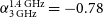 $\alpha_{3\,{\rm GHz}}^{1.4\,{\rm GHz}}=-0.78$. Potentially this up-turn could be indicative of a boosted radio emission from the core, expected for type 1 AGN. Or more likely it could simply be statistical uncertainty as the higher frequency spectral index is determined over a relatively narrow frequency range.
Our selection relies on low-frequency spectral curvature which is only possible from the broadband coverage of the MWA. This curvature is either due to synchrotron self-absorption processes or possibly free-free absorption from the host galaxy or circum-galactic medium. We note that PSO J352.4034-15.3373 does not show the low-frequency curvature seen in our sample which could be due to its selection as an unobscured type 1 galaxy.
No systematic CO follow-up campaigns of samples of  $z>5$ quasars exist as the low-J CO lines are redshifted outside of ALMA Band 3. We therefore compare qualitatively the 0856 properties to some smaller samples or individual objects. When compared to the hyper-luminous obscured quasars sample from Fan et al. (Reference Fan, Knudsen, Fogasy and Drouart2018), 0856 appears relatively similar in term of CO brightness, but maybe on the higher side when compared to line width. If compared with bright sub-mm galaxies, such as the sample presented in Weiß et al. (Reference Weiß2013) and comparing the CO brightness corrected from magnification, 0856 appears also similar. A comparison with the gas-rich star-forming galaxies from Tacconi et al. (Reference Tacconi2010) indicates that 0856 CO brightness is in the higher end of the sample. Finally, if compared to some sources of the HeRGÉ sample (Emonts et al. Reference Emonts2014; Gullberg et al. Reference Gullberg2016), our derived CO brightnesses are a factor of few fainter, but this is mainly due to the sensitivity limit of the low-J CO surveys performed with ATCA.
6. Conclusions
We have presented a new and efficient method to identify and confirm powerful radio-loud AGN at  $z>5$ by taking advantage of the new, low-frequency, all-sky GLEAM survey. We made use of the large frequency coverage (70–230 MHz) to select sources from their spectral index and curvature. In our pilot project, we followed up our best candidates in the G09 field with VLT/HAWK-I, ATCA, and ALMA. Out of our four sources, we successfully detected a source at
  $z=5.55$ and presented a very tentative candidate at
  $z=10.15$, which requires additional data for a robust confirmationFootnote e. Hence, the efficiency of our method of finding
  $z>5.5$ radio galaxies is in the 25–50% range (albeit from small number statistics).
From their radio luminosities, it appears clear that we preferentially select the most powerful radio sources, very similar to the already existing HeRGÉ sample ( $\text{L}_{\rm 500\,MHz}>10^{27}\,\text{W\,Hz}^{-1}$ Seymour et al. Reference Seymour2007). Their faint
  $K_s$ magnitude (preferably selecting obscured type 2 AGN) place our object in the K–z relation, known to pinpoint to the most massive system as any redshift, and consistent with
 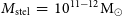 ${M}_{\rm stel}\,=\,10^{11-12}{\rm M}_{\odot}$ elliptical galaxies (Rocca-Volmerange et al. Reference Rocca-Volmerange, Le Borgne, De Breuck, Fioc and Moy2004). Moreover, as we suspect these galaxies harbour the most massive black holes, finding and confirming the redshifts of a larger sample of such sources could in the future present tight constraints on galaxy formation scenarios (e.g. Haiman Reference Haiman2004; Volonteri & Rees Reference Volonteri and Rees2005).
Our method shows that spectroscopy of bright molecular lines will be our only way to confirm routinely the redshift of these sources which are intrinsically fainter in  $K_s$-band before the era of 30-m class telescopes and the James Webb Space Telescope. The hunt for powerful radio galaxies within the EoR continues.
Acknowledgements
GD would like to thank Maria Strandet for her very useful and valuable input on the ALMA spectral extraction and interpretation and Jess Broderick for his careful reading. GD received the support of the ESO Scientific Visitor Programme.
JA acknowledges financial support from the Science and Technology Foundation (FCT, Portugal) through research grants PTDC/FIS-AST/29245/2017, UID/FIS/04434/2013, and UID/FIS/04434/2019.
The National Radio Astronomy Observatory is the facility of the National Science Foundation operated under cooperative agreement by Associated Universities, Inc.
This paper makes use of the following ALMA data: ADS/JAO.ALMA#2017.1.00719.S. ALMA is a partnership of ESO (representing its member states), NSF (USA), and NINS (Japan), together with NRC (Canada), MOST and ASIAA (Taiwan), and KASI (Republic of Korea), in cooperation with the Republic of Chile. The Joint ALMA Observatory is operated by ESO, AUI/NRAO, and NAOJ.
Based on observations made with ESO Telescopes at the La Silla Paranal Observatory under programme ID 0101.A-0571(A). GD would like to thank the user support department at ESO with the help provided with the HAWK-I pipeline.
This scientific work makes use of the Murchison Radio Astronomy Observatory, operated by CSIRO. We acknowledge the Wajarri Yamatji people as the traditional owners of the Observatory site.
The Australia Telescope Compact Array is part of the Australia Telescope National Facility which is funded by the Australian Government for operation as a National Facility managed by CSIRO.
GAMA is a joint European-Australasian project based around a spectroscopic campaign using the Anglo-Australian Telescope. The GAMA input catalogue is based on data taken from the Sloan Digital Sky Survey and the UKIRT Infrared Deep Sky Survey. Complementary imaging of the GAMA regions is being obtained by a number of independent survey programmes including GALEX MIS, VST KiDS, VISTA VIKING, WISE, Herschel-ATLAS, GMRT, and ASKAP providing UV to radio coverage. GAMA is funded by the STFC (UK), the ARC (Australia), the AAO, and the participating institutions. The GAMA website is http://www.gama-survey.org/. Based on observations made with ESO Telescopes at the La Silla Paranal Observatory under programme ID 179.A-2004.
This research has made use of astropy,Footnote f a community-developed core Python package for Astronomy (Collaboration et al. Reference Collaboration2013, Reference Collaboration2018).
This research has made use of NASA Astrophysics Data System.
Facilities: ALMA, ATCA, JVLA, MWA, VISTA, VLT.
Software: astropy, casa, eazy, MrMoose, numpy, scipy, sofia, sslf.
A. Appendix
A.1. GLEAM IDR3 vs the public data release
Our initial source selection was based on the IDR3 version of the GLEAM extra-galactic catalogue available to the MWA consortium. If we apply our selection criteria (described in Section 2) to the public catalogue, we obtain 71 sources (compared to 52) with 28 of each sample overlapping. The principle difference between the samples as a whole when we perform the MWA SED fitting is that the public data have on average an offset  $\delta\beta=-0.3$ compared to IDR3. Hence, public sources will enter our selection criteria and some IDR3 sources will leave it (this is the case for 0856 and 0917). Hence, the MWA sources are measured to be more curved in the public release than in IDR3. This can be explained by the lower frequency fluxes (
 $\nu<110\,\text{MHz}$) being fainter by up to 20% in the public release (due to the improvements in data calibration and processing and a better characterisation of the related uncertainties). For this reason, we recommend using a lower
  $\beta$ interval to reproduce our selection with the public release (e.g.
  $-1.4<\beta<-0.6$). Our highest redshift candidates, 0856 and 0917, are recovered with these parameters. Note that the track for 8C 1435+635 will not move as the curvature of this Northern hemisphere source is not defined by GLEAM data.


