


1. Introduction
Thermal convection manifests not only in various geophysical and astrophysical systems, but also in smaller-scale phenomena ranging from industrial processes to our daily lives such as household heating. One of the classical and probably the most intensively investigated configurations of natural thermal convection is Rayleigh–Bénard convection (RBC) (Bodenschatz, Pesch & Ahlers Reference Bodenschatz, Pesch and Ahlers2000; Ahlers, Grossmann & Lohse Reference Ahlers, Grossmann and Lohse2009; Chillà & Schumacher Reference Chillà and Schumacher2012). In RBC, the heated and cooled surfaces are placed orthogonal to the gravity vector, and the fluid layer is heated from below and cooled from above. Thermal expansion causes warm fluid to rise and cool fluid to sink. At sufficiently large Rayleigh number  ${{Ra}}\equiv \alpha g\varDelta H^3 / (\kappa \nu )$, the resulting turbulent convective flow self-organises through an inverse energy cascade from small-scale thermal turbulence to large flow structures. Here, $\alpha$ is the isobaric thermal expansion coefficient, $\nu$ is the kinematic viscosity, $\kappa$ is the thermal diffusivity, $\varDelta$ is the temperature difference between the heated and cooled surfaces, $H$ is the distance between these surfaces (i.e. the height of the container), and $g$ denotes the acceleration due to gravity. Investigation of thermal convection in low-Prandtl-number fluids (Prandtl numbers ${{Pr}} \ll 1$) is of particular importance for a better understanding of convection on the surfaces of stars, where ${{Pr}}$ can be as low as $10^{-8}$, and in the case of liquid metals, for numerous technical applications, e.g. the advancement of cooling technology (see e.g. Frick et al. Reference Frick, Khalilov, Kolesnichenko, Mamykin, Pakholkov, Pavlinov and Rogozhkin2015; Schumacher, Götzfried & Scheel Reference Schumacher, Götzfried and Scheel2015; Scheel & Schumacher Reference Scheel and Schumacher2016; Teimurazov & Frick Reference Teimurazov and Frick2017; Teimurazov, Frick & Stefani Reference Teimurazov, Frick and Stefani2017; Zürner et al. Reference Zürner, Schindler, Vogt, Eckert and Schumacher2019; Zwirner et al. Reference Zwirner, Khalilov, Kolesnichenko, Mamykin, Mandrykin, Pavlinov, Shestakov, Teimurazov, Frick and Shishkina2020a, Reference Zwirner, Emran, Schindler, Singh, Eckert, Vogt and Shishkina2022; Pandey et al. Reference Pandey, Krasnov, Sreenivasan and Schumacher2022).
In RBC, at sufficiently large  ${{Ra}}$, the flow is self-organised into a large-scale circulation (LSC), or a turbulent thermal wind, the concept of which is an important ingredient in the heat and momentum transport theory (Grossmann & Lohse Reference Grossmann and Lohse2000, Reference Grossmann and Lohse2001, Reference Grossmann and Lohse2011), and boundary-layer theory for natural thermal convection (Shishkina et al. Reference Shishkina, Horn, Wagner and Ching2015; Ching et al. Reference Ching, Leung, Zwirner and Shishkina2019; Tai et al. Reference Tai, Ching, Zwirner and Shishkina2021). The resulting flow structures depend strongly on the Rayleigh number ${{Ra}}$, which is a measure of the thermal forcing that drives convection in the system, and on the Prandtl number ${{Pr}}\equiv \nu /\kappa$, which describes the diffusive properties of the considered fluid. In addition, the geometric characteristics of the container, especially the shape of the container and, in particular, the aspect ratio $\varGamma$ of its spatial length $L$ and height $H$,
$H$,  $\varGamma \equiv L/H$, influence the global flow structure and the mean characteristics of the flow (Shishkina Reference Shishkina2021; Ahlers et al. Reference Ahlers2022).
Turbulent RBC in a cylindrical container with equal height and diameter (aspect ratio  $\varGamma =1$) is the most extensively studied. For containers with $\varGamma \approx 1$, the principal structure of the LSC can be delineated as follows. There exists a vertical plane (called the LSC plane), in which the LSC is observed as a big domain-filling roll with two smaller secondary rolls in the corners, while in the orthogonal vertical plane, the LSC for this geometry of the container is seen as a four-roll structure, with an inflow at mid-height (Shishkina, Wagner & Horn Reference Shishkina, Wagner and Horn2014). Not only is the LSC generally unsteady, but also the LSC path can exhibit dynamic behaviour. Thus in containers with $\varGamma \approx 1$, the LSC can display various modes of periodic or chaotic oscillations that can take the form of sloshing, precession and torsion (Cioni, Ciliberto & Sommeria Reference Cioni, Ciliberto and Sommeria1997; Funfschilling & Ahlers Reference Funfschilling and Ahlers2004; Xi, Lam & Xia Reference Xi, Lam and Xia2004; Sun, Xia & Tong Reference Sun, Xia and Tong2005; Brown & Ahlers Reference Brown and Ahlers2006, Reference Brown and Ahlers2007; Xi & Xia Reference Xi and Xia2007, Reference Xi and Xia2008; Funfschilling, Brown & Ahlers Reference Funfschilling, Brown and Ahlers2008; Zhou et al. Reference Zhou, Xi, Zhou, Sun and Xia2009; Sugiyama et al. Reference Sugiyama, Ni, Stevens, Chan, Zhou, Xi, Sun, Grossmann, Xia and Lohse2010; Assaf, Angheluta & Goldenfeld Reference Assaf, Angheluta and Goldenfeld2011; Stevens, Clercx & Lohse Reference Stevens, Clercx and Lohse2011; Wagner, Shishkina & Wagner Reference Wagner, Shishkina and Wagner2012; Sakievich, Peet & Adrian Reference Sakievich, Peet and Adrian2020; Cheng et al. Reference Cheng, Mohammad, Wang, Keogh, Forer and Kelley2022). The sloshing mode is associated with the motion of the LSC plane in the radial direction, while the precession and torsion modes are related to the azimuthal motion of the LSC plane (Horn, Schmid & Aurnou Reference Horn, Schmid and Aurnou2021; Cheng et al. Reference Cheng, Mohammad, Wang, Keogh, Forer and Kelley2022). In the precession mode, the entire LSC plane drifts in the azimuthal direction, while in the torsion mode, the azimuthal motion of the LSC plane in the upper half of the container is generally in the direction opposite to the motion of the LSC plane in the lower half of the container.
In slender containers with aspect ratio  $\varGamma <1$, a single big-roll structure of the LSC is not as stable as in the case $\varGamma =1$ (Xi & Xia Reference Xi and Xia2008; Weiss & Ahlers Reference Weiss and Ahlers2011, Reference Weiss and Ahlers2013; Zwirner, Tilgner & Shishkina Reference Zwirner, Tilgner and Shishkina2020b; Schindler et al. Reference Schindler, Eckert, Zürner, Schumacher and Vogt2022). For $\varGamma <1$, the turbulent LSC can be formed of several dynamically changing convective rolls that are stacked on top of each other (van der Poel et al. Reference van der Poel, Stevens, Sugiyama and Lohse2012; Zwirner et al. Reference Zwirner, Tilgner and Shishkina2020b). The mechanism that causes the twisting and breaking of a single-roll LSC into multiple rolls is the elliptical instability (Zwirner et al. Reference Zwirner, Tilgner and Shishkina2020b). In the case $\varGamma <1$, the heat and momentum transports, which are represented by the Nusselt number ${{Nu}}$ and Reynolds number $Re$, are always stronger for a smaller number of the rolls that form the LSC. This was proven in experiments for $\varGamma =1/2$ (Xi & Xia Reference Xi and Xia2008; Weiss & Ahlers Reference Weiss and Ahlers2011, Reference Weiss and Ahlers2013), and simulations for $\varGamma =1/5$ (Zwirner & Shishkina Reference Zwirner and Shishkina2018; Zwirner et al. Reference Zwirner, Tilgner and Shishkina2020b).
By contrast, for wide containers with  $\varGamma > 1$, the more rolls of the LSC mean the more efficient heat transport (van der Poel et al. Reference van der Poel, Stevens, Sugiyama and Lohse2012; Wang et al. Reference Wang, Verzicco, Lohse and Shishkina2020), also in highly turbulent cases. For $\varGamma > 1$, the rolls or roll-like structures are attached to each other and aligned in horizontal directions (Hartlep, Tilgner & Busse Reference Hartlep, Tilgner and Busse2003; von Hardenberg et al. Reference von Hardenberg, Parodi, Passoni, Provenzale and Spiegel2008; Emran & Schumacher Reference Emran and Schumacher2015). In the two-dimensional case, the range of possible aspect ratios of particular convective rolls, and hence the total number of the rolls in any confined domain, are restricted, and there exist quite accurate theoretical estimates for the lower and upper bounds of possible aspect ratios of the rolls (Wang et al. Reference Wang, Verzicco, Lohse and Shishkina2020; Shishkina Reference Shishkina2021).
For three-dimensional domains, the typical length scales of the self-organised coherent turbulent flow structures are not yet well-studied, and their accurate prediction remains an unsolved problem so far. These flow structures can be identified as turbulent superstructures (Pandey, Scheel & Schumacher Reference Pandey, Scheel and Schumacher2018; Stevens et al. Reference Stevens, Blass, Zhu, Verzicco and Lohse2018; Green et al. Reference Green, Vlaykov, Mellado and Wilczek2020; Krug, Lohse & Stevens Reference Krug, Lohse and Stevens2020; Berghout, Baars & Krug Reference Berghout, Baars and Krug2021), since their lifetime is much larger than the free-fall time, and their length scales are generally larger than the typical length scale in RBC, which is the height of the container  $H$. Several studies suggest that the characteristic length scale of these coherent turbulent large-scale flow structures increases with growing ${{Ra}}$; see e.g. Hartlep et al. (Reference Hartlep, Tilgner and Busse2003), Pandey et al. (Reference Pandey, Scheel and Schumacher2018), Akashi et al. (Reference Akashi, Yanagisawa, Tasaka, Vogt, Murai and Eckert2019) and Krug et al. (Reference Krug, Lohse and Stevens2020). Depending on the considered parametric space of ${{Ra}}$, ${{Pr}}$ and $\varGamma$ in different studies, different preferable length scales of the turbulent superstructures are reported, which are always larger that the container height $H$. Thus the values of order $10H$ (Busse Reference Busse1994), or between $6H$ and $7H$ (Hartlep et al. Reference Hartlep, Tilgner and Busse2003; Pandey et al. Reference Pandey, Scheel and Schumacher2018; Stevens et al. Reference Stevens, Blass, Zhu, Verzicco and Lohse2018), were proposed. Although the typical horizontal wavelengths of the turbulent superstructures generally grow with ${{Ra}}$, they tend to decrease with decreasing Prandtl number (Pandey et al. Reference Pandey, Scheel and Schumacher2018). This fact is pretty remarkable, since decreasing ${{Pr}}$ is usually associated with even stronger turbulence, therefore one might expect a certain similarity to the situation when ${{Ra}}$ is increased.
Recent laboratory and numerical experiments show that in an intermediate range of moderate aspect ratios,  $\varGamma \gtrsim 1.4$, the LSC displays a low-frequency oscillatory dynamics (Vogt et al. Reference Vogt, Horn, Grannan and Aurnou2018; Horn et al. Reference Horn, Schmid and Aurnou2021; Akashi et al. Reference Akashi, Yanagisawa, Sakuraba, Schindler, Horn, Vogt and Eckert2022; Cheng et al. Reference Cheng, Mohammad, Wang, Keogh, Forer and Kelley2022). The precession, sloshing and torsional (ST) dynamics of the LSC, which dominates at $\varGamma =1$, is replaced by a mode that can be described as a jump rope vortex (JRV). In this flow pattern, a curved vortex is formed, which swirls around the cell centre in the direction opposite to the LSC direction, resembling the motion of a swirling jump rope; see figure 1(e). This phenomenon was first demonstrated for liquid-metal convection in a cylinder with aspect ratio $\varGamma =2$ (Vogt et al. Reference Vogt, Horn, Grannan and Aurnou2018). Numerical simulations showed that the JRV exists also for a cylindrical container of the aspect ratio $\varGamma =\sqrt {2}$, and that the JRV structure is present not only in low- ${{Pr}}$ liquid-metal convection, but also in water at ${{Pr}} = 4.38$ (Vogt et al. Reference Vogt, Horn, Grannan and Aurnou2018). This has been confirmed in several other experiments and simulations of comparable aspect ratios for both water and liquid metal (Horn et al. Reference Horn, Schmid and Aurnou2021; Cheng et al. Reference Cheng, Mohammad, Wang, Keogh, Forer and Kelley2022; Li et al. Reference Li, Chen, Xu and Xi2022). However, no JRV was detected in a $\varGamma = 3$ cylinder (Cheng et al. Reference Cheng, Mohammad, Wang, Keogh, Forer and Kelley2022).

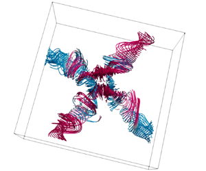
Figure 1. Phase-averaged streamlines in RBC for  ${{Pr}}=0.03$, ${{Ra}}=10^6$, as obtained in direct numerical simulations for different aspect ratios (a) $\varGamma =5$, (b) $\varGamma =3$, (c) $\varGamma =2.5$, (d) $\varGamma =2$ (box) for square cuboid domains (new simulations) and (e) $\varGamma =2$ (cylinder), adapted from Vogt et al. (Reference Vogt, Horn, Grannan and Aurnou2018), available under CC BY-NC-ND 4.0. These streamlines envelop the oscillating vortex, and the colour scale is according to the vertical velocity component $u_z$. Blue (red) corresponds to a negative (positive) value of $u_z$, indicating a downward (upward) direction of the flow. The structures in the lower-aspect-ratio cases ( $\varGamma =2$, 2.5 and 3) are building units of the structure formed within the largest-aspect-ratio case ( $\varGamma =5$).
Flow measurements in containers of different shapes, such as a cuboid domain with  $\varGamma = 5$ (Akashi et al. Reference Akashi, Yanagisawa, Sakuraba, Schindler, Horn, Vogt and Eckert2022), showed that the strongly oscillating velocity and temperature fields could also be attributed to the presence of the JRV-like structures. However, instead of only one vortex, four JRVs interlaced in that case. The ends of the JRVs cross perpendicularly at a certain point in space (see figure 1a). Here, the detached (opposite) JRVs oscillate ${\rm \pi}$ out of phase, whereas adjacent JRVs do so with a lag of ${\rm \pi} /2$. Akashi et al. (Reference Akashi, Yanagisawa, Sakuraba, Schindler, Horn, Vogt and Eckert2022) demonstrated that the JRVs can form a lattice structure of different vortices, which determines a fundamental flow mode that for the considered combinations of ${{Ra}}$ and ${{Pr}}$ can dominate the dynamics at moderate, and possibly also very large, aspect ratios.
Although JRVs have also been detected in water with moderate  ${{Pr}} \approx 5$, the liquid metal offers a number of advantages for such studies. The velocity field in liquid-metal convection is strongly inertia dominated due to its low viscosity and high density. As a result, the JRV-induced oscillations reach much stronger amplitudes than in water or air. While the velocity field in low- ${{Pr}}$ liquid metal at comparable temperature gradients is significantly more turbulent than that of water or air, the temperature field exhibits considerably more coherence than the velocity field due to the large thermal diffusivity. Thus the JRV-induced oscillations can be detected very well both in the velocity field and in the temperature field. As such, liquid metals are well suited to investigate the JRV-like flow dynamics.
The objective of the present work is to investigate in more detail the aspect ratio and geometry dependence of the three-dimensional oscillatory JRV-like LSC in liquid-metal thermal convection. In particular, we investigate how increasing aspect ratios result in a lattice of oscillatory flow pattern via the formation of JRVs, starting from the smallest structural building block to that of the more interlaced JRVs at a higher aspect ratio. To this end, we study the LSC dynamics in RBC of liquid metal with  ${{Pr}}=0.03$ in square cuboids with different aspect ratios, which vary from 2 to 5, using both experimental and numerical approaches. Table 1 summarises previous studies and our present work to highlight the gap our study fills. For the first time, we investigate the dominant oscillation modes of the LSC in cuboids with $\varGamma = 2$, 2.5 and 3. For the case $\varGamma = 5$, we extended the parameter range compared to Akashi et al. (Reference Akashi, Yanagisawa, Sakuraba, Schindler, Horn, Vogt and Eckert2022) by increasing ${{Ra}}$ and the numerical resolution.
Table 1. Details on the type of LSC observed for different control parameters.

2. Methods
2.1. Direct numerical simulations
Thermal convection under the assumption of the Oberbeck–Boussinesq approximation is described by the following Navier–Stokes, energy and continuity equations:
 \begin{gather} D_t \boldsymbol{u} = \nu\,{\nabla}^2 \boldsymbol{u} - \boldsymbol{\nabla} p + \alpha g (T-T_0) \boldsymbol{e}_z, \end{gather}
 \begin{gather}D_t T = \kappa\,{\nabla}^2 T, \end{gather}
 \begin{gather}\boldsymbol{\nabla} \boldsymbol{\cdot} \boldsymbol{u} = 0. \end{gather}
Here,  $D_{t}$ denotes the substantial derivative, $\boldsymbol {u} = (u_x, u_y, u_z)$ is the velocity vector field, $p$ is the reduced kinematic pressure, $T$ is the temperature, $T_0=(T_++T_-)/2$ is the arithmetic mean of the top ( $T_-$) and bottom ( $T_+$) temperatures, and $\boldsymbol {e}_z$ is the unit vector that points upwards. The considered domain is a square cuboid with the height $H$ and equal width $W$ and length $L$,
$L$,  $W=L$, so that the domain aspect ratio equals $\varGamma \equiv L/H$. The system (2.1)–(2.3) is closed by the following boundary conditions: no-slip for the velocity at all boundaries, $\boldsymbol {u}=0$; constant temperatures at the end face of the box, i.e. $T=T_+$ at the bottom plate at $z=0$, and $T=T_-$ at the top plate at $z=H$; and adiabatic boundary condition at the sidewalls, $\partial T/\partial \boldsymbol {n}=0$, where $\boldsymbol {n}$ is the vector orthogonal to the surface. Equations (2.1)–(2.3) are non-dimensionalised by using the height $H$, the free-fall velocity $u_{f\!f}$, the free-fall time $t_{f\!f}$, and the temperature difference between the heated plate and the cooled plate, $\varDelta$,
 \begin{equation} u_{f\!f}\equiv(\alpha gH\varDelta)^{1/2},\quad t_{f\!f}\equiv H/u_{f\!f},\quad \varDelta\equiv T_+ - T_-, \end{equation}
as units of length, velocity, time and temperature, respectively.
The resulting dimensionless equations are solved numerically using the latest version (Reiter et al. Reference Reiter, Shishkina, Lohse and Krug2021; Reiter, Zhang & Shishkina Reference Reiter, Zhang and Shishkina2022) of the direct numerical solver Goldfish (Shishkina et al. Reference Shishkina, Horn, Wagner and Ching2015; Kooij et al. Reference Kooij, Botchev, Frederix, Geurts, Horn, Lohse, van der Poel, Shishkina, Stevens and Verzicco2018), which applies a fourth-order finite-volume discretisation on staggered grids. Three-dimensional direct numerical simulations (DNS) were performed for square cuboid domains with the aspect ratios  $\varGamma = 2$, 2.5, 3 and 5. The utilised staggered computational grids, which are clustered near all rigid walls, are sufficiently fine to resolve the Kolmogorov microscales (Shishkina et al. Reference Shishkina, Stevens, Grossmann and Lohse2010); see tables 2 and 3.
Table 2. Details on the conducted DNS, including the numbers of nodes  $N_x$, $N_y$, $N_z$ in the directions $x$,
$x$,  $y$ and $z$, respectively; the number of the nodes within the thermal boundary layer, $\mathcal {N}_{\theta }$, and within the viscous boundary layer, $\mathcal {N}_{v}$; the relative thickness of the thermal boundary layer, $\delta _{\theta }/H$, and the viscous boundary layer $\delta _{v}/H$; the Kolmogorov microscale $h_{K}$, and the relative mean grid stepping $h_{DNS}/h_{K}$.

Table 3. Details on the conducted DNS and experiments.

2.2. Experimental set-up
A schematic of the experimental set-up is presented in figure 2 along with the measuring positions of ultrasound probes. The set-up consists of a cuboid vessel with base area  $L\times L=200 \times 200\,\mathrm {mm}^2$ and height $H=66$ mm, resulting in aspect ratio $\varGamma \approx 3$. The top and bottom plates of this vessel are made of copper, whereas the sidewalls are made of polyvinyl chloride (PVC) of 30 mm thickness. This vessel is filled with a eutectic liquid-metal alloy GaInSn of gallium, indium and tin, which serves as the working fluid in the experiment. Thermophysical properties of GaInSn are reported in Plevachuk et al. (Reference Plevachuk, Sklyarchuk, Eckert, Gerbeth and Novakovic2014). In particular, the melting point of GaInSn is $10.5\,^\circ \text {C}$, and the Prandtl number is ${{Pr}} \approx 0.03$.

Figure 2. Schematics of the experimental set-up: (a–c) three projections showing (a) the top view and (b,c) two side views; and (d) a three-dimensional sketch, illustrating the positions of all ultrasound transducers. Each ultrasound transducer is marked with a letter that indicates the distance to the bottom (‘T’ – close to the top, ‘M’ – matching the middle plane, ‘B’ – close to the bottom) followed by a number. All dimensional distances in (a–c) are given in mm. Blue and red colours indicate the cooled and heated plates, respectively.
The liquid layer enclosed within the vessel is heated from the bottom and cooled from the top by adjusting the temperature of water flowing through channels in the copper plates. The temperature of water in these channels is held constant at set temperatures via two external thermostats. To minimise heat losses, the tubes transporting the hot and cold water and the entire vessel are wrapped in about 30 mm thick insulating foam tubes and additional envelope. Two platinum resistance thermometers (Pt-100) (accuracy  ${\pm }0.005$ K) have been utilised to monitor accurately the temperatures of water entering ( $T_{in}$) and leaving ( $T_{out}$) the hot and cold plates, respectively. These temperature readings are essential in measuring the non-dimensional convective heat transport, the Nusselt number ${{Nu}}$, expressed as ${{Nu}}=\dot {\varPhi }/\dot {\varPhi }_{cond}$. Here, $\dot {\varPhi }_{cond}=\lambda L^2 \varDelta / H$ is the conductive heat flux, with $\lambda$ being the thermal conductivity of the liquid metal, and $\dot {\varPhi }=\rho c_p \dot {V} (T_{in}-T_{out})$ is the total heat flux exchanged in the set-up, whereas $c_p$ is the isobaric heat capacity of water, and $\dot {V}$ is the flow rate of the circulating water determined via an axial turbine flow sensor at the cooling outlet of the set-up.
Prior to measurements, calibrations are performed. To account for the measurement uncertainty and heat losses of the set-up, hose split valves are used to split cold and hot water outlets, respectively. One set of a cold and hot pair is used to feed the top plate, and the other set to feed the bottom plate, while ensuring that the temperature of both the plates remained at a set temperature  $20\,^\circ \text {C}$ using the external thermostats. Once the temperature in the plates reaches an equilibrium, an hour-long time series of temperature readings from both sets of thermocouples is recorded. Using the least squares method, offsets from each of these thermocouples are extracted, which are then used to correct the temperature measurements. This procedure gives a lower threshold of temperature difference attainable for the set-up; measurements below $\varDelta \leq 0.22\,^\circ \text {C}$ are untenable. The range of measured temperature difference realised in this set-up was $0.27\,^\circ \text {C} \leq \varDelta \leq 16\,^\circ \text {C}$, with Rayleigh number in the range $2.9 \times 10^4 \leq Ra \leq 1.6 \times 10^6$. Experimental results presented here (see table 3) are recorded after the temperature difference between the hot and the cold plates reached a constant value, when the system attains thermal equilibrium.
Principles of ultrasound Doppler velocimetry (UDV), a technique used widely for opaque flow diagnostics, are implemented to determine the fluid velocity (Tsuji et al. Reference Tsuji, Mizuno, Mashiko and Sano2005; Eckert, Cramer & Gerbeth Reference Eckert, Cramer and Gerbeth2007). Nine UDV transducers (TR0805SS, Signal Processing SA) are installed in direct contact with the fluid. Each of these transducers acquires an instantaneous velocity profile sequentially along the measuring lines as shown in figure 2 using multiplexing. The velocity measurements are performed with resolution approximately  $0.5\,{\rm mm}\,{\rm s}^{-1}$ and sampling frequency 1 Hz.
For the numerical results, statistical equilibrium or convergence is reached after several hundreds of free-fall time units. Throughout this paper, the length, velocity and time are made non-dimensional using the cell height  $H$, the free-fall velocity $u_{f\!f}$, and the free-fall time unit $t_{f\!f}\equiv H/u_{f\!f}$, respectively; see (2.4a–c).
2.3. Phase averaging procedure
To analyse the three-dimensional flow dynamics from the experimental data, the whole field mapping of the velocity flow field is required, which is currently not possible using the UDV techniques. However, this sort of flow-field measurements can be assessed via the numerical techniques. The flow pattern consists of oscillatory coherent structures over several range of scales. To visualise the coherent structures, it is advisable to remove the background turbulent fluctuations using statistical means. Pandey et al. (Reference Pandey, Scheel and Schumacher2018) implemented an averaging method, which was later adopted by Akashi et al. (Reference Akashi, Yanagisawa, Sakuraba, Schindler, Horn, Vogt and Eckert2022) in the form of a phase averaging algorithm. In this algorithm, one complete oscillation period,  $\tau _{OS}= 1/f_{OS}$, is equally divided into certain (e.g. 16) intervals or phases. Averaging of the temperature and velocity field data is carried out within each of these phases. This method reveals the underlying coherent structures in a flow field with high oscillations, such as that encountered in the three-dimensional cellular regime by Akashi et al. (Reference Akashi, Yanagisawa, Sakuraba, Schindler, Horn, Vogt and Eckert2022).
Vogt et al. (Reference Vogt, Horn, Grannan and Aurnou2018) used conditional averaging to showcase the three-dimensional structures of the JRVs in a cylinder. The method of conditional averaging is similar to that of the phase averaging process, with the only difference in the choice of the conditioning intervals. In the conditional averaging approach, the intervals for one complete cycle are divided into seven intervals bounded by multiples of standard deviations of the average temperature of the fluid.
In the present study, the phase averaging method is applied to the simulation data, which cover 16 oscillation periods for the cases  $\varGamma = 2.5$, $3$,
$3$,  $5$ and 8 oscillation periods for the case $\varGamma = 2$. Every oscillation period is divided into 16 phases, and each phase is represented by 20 snapshots of all flow fields. Then the corresponding snapshots are averaged within each phase. Finally, the conditional averaging is applied to the flow fields within each phase and for all oscillation periods, which gives a phase-averaged temporal evolution of all flow fields during the period.
3. Results
The results of all conducted DNS and experiments are summarised in table 3. For all experimental and numerical data for sufficiently large  ${{Ra}}$, an oscillatory behaviour of the LSC was identified. As in the cases $\varGamma =\sqrt {2}$ and $2$ of a cylindrical container (Vogt et al. Reference Vogt, Horn, Grannan and Aurnou2018), the JRV-like oscillatory structures leave imprints on almost all flow characteristics, for the considered ranges of ${{Ra}}$ and $\varGamma$ of a cuboid domain. The oscillatory behaviour of the LSC is reflected in temporal evolution of the temperature and particular components of the velocity fields, and is also seen in the vertical heat flux temporal evolution. Here, we are focusing on the cases of higher ${{Ra}}$ with the JRV dominance, rather than on cases of lower ${{Ra}}$, where unsteady convection rolls are dominant and JRVs are absent. Transition from convection rolls to large-scale cellular structures with JRV in turbulent RBC with increasing ${{Ra}}$ for $\varGamma =5$ is described in detail in Akashi et al. (Reference Akashi, Yanagisawa, Tasaka, Vogt, Murai and Eckert2019).
Once the dominating frequency  $f_0$ is evaluated (we will discuss this in more detail later), one can analyse the mean flow dynamics within the time period that lasts $\tau _{OS}= 1/f_0$. For that, the temporal evolution of the flow fields, which are obtained in the DNS, are split into separate periods, according to the dominating frequency $f_0$, then a phase-averaged temporal evolution of all flow fields during the period is calculated.
Our DNS for  ${{Ra}} = 10^6$ and ${{Pr}} = 0.03$, and two different aspect ratios, $\varGamma =5$ and $2.5$, show a very remarkable similarity of the global flow structure and its dynamics. In figure 3, phase-averaged instantaneous temperature distributions in horizontal cross-sections are presented, which are considered at distances $z= 0.5H$ (figures 3a,b,e,f) and $z= 0.85H$ (figures 3c,d,g,h) from the bottom plate, and at the times $t=0$ and $0.5\tau _{OS}$. This figure shows patches of upwelling (hot) and downwelling (cold) fluid, with the hot patches connected by a diagonal ridge of upwelling fluid. These patches rotate anticlockwise in the time interval $[0,0.5\tau _{OS}]$ (see supplementary movie 1), suggesting the presence of oscillatory flow dynamics that periodically changes the flow topology. For fixed values of ${{Ra}}$ and the cell height $H$, the spatial length of the convection cell in the case $\varGamma =5$ is twice as large as in the case $\varGamma =2.5$ for the same ${{Ra}}$ and $H$. Therefore, for any fixed $z$, one can expect a similarity of the flow pattern in the horizontal cross-section at the height $z$ in the case $\varGamma =2.5$ with the flow pattern in the $1/4$ of the area of the horizontal cross-section at the same height $z$ in the case $\varGamma =5$. Indeed, figure 3 shows that the temperature distribution in the region marked with black dashed lines for $\varGamma =5$ (figures 3a–d) is very similar to the temperature distribution in the corresponding cross-sections for $\varGamma =2.5$ (figures 3e–h) if considered at the same phase.

Figure 3. Phase-averaged snapshots of the temperature at a distance  $z$ from the bottom: (a,b,e,f) $z= 0.5H$, and (c,d,g,h) $z=0.85H$, for different container aspect ratios (a–d) $\varGamma = 5$ and (e–h) $\varGamma = 2.5$, as obtained in the simulations for ${{Ra}} = 10^6$ and ${{Pr}} = 0.03$ (see supplementary movie 1 available at https://doi.org/10.1017/jfm.2023.936). The virtual probe lines T1 and T2 (see also figure 4) are indicated with dashed white lines. The black squares indicate the areas that correspond to the areas of the container with $\varGamma =2.5$.
To gain more evidence for this similarity, we evaluate the horizontal components of the velocity,  $u_y$ and $u_x$, along the lines marked T1 and T2 in figures 3(c,d) ( $\varGamma =5$) and compare them with the corresponding horizontal components of the velocity along the lines marked T1 and T2 in figures 3(g,h) ( $\varGamma =2.5$). The temporal evolutions of these velocity components for $\varGamma =5$ and $2.5$ are compared in figure 4 for ${{Ra}} = 10^6$ and $z= 0.85H$. One can see that the lower halves of the spatio-temporal velocity maps in figures 4(a,b), which correspond to the measurements along the lines T1 and T2 within the $1/4$ area that is marked in figures 3(c,d) with the black dashed lines, mimic the spatio-temporal velocity maps in figures 4(c,d), which correspond to the measurements along the lines T1 and T2 in figures 3(g,h).

Figure 4. Spatio-temporal velocity maps for  ${{Ra}} = 10^6$ at $z= 0.85H$, as obtained in the DNS at the virtual probe lines (a,c) T1 and (b,d) T2, for the aspect ratios (a,b) $\varGamma =5$ and (c,d) $\varGamma = 2.5$. The black dashed lines in (a,b) correspond to the measurements in the cuboid with $\varGamma =2.5$ (c,d), respectively.
Qualitatively, the signals for  $\varGamma = 5$ and $2.5$ are similar; however, the frequency of the oscillations in the latter case is slightly lower than that in the former case, with six versus five oscillations during the same time interval. Also, at $\varGamma = 5$, the signal seems to be less stable than in the case $\varGamma = 2.5$.
Figure 5 shows a comparison of the experimental and simulation results for the same  $\varGamma =3$ and ${{Ra}}=10^6$. Here, a comparison of the temporal evolution of the horizontal components of the velocity is made at exactly the same locations in the DNS and in the experiment. One can see good qualitative agreement between the experimental and simulation data. However, the dominant frequency obtained in the experiment is slightly higher compared to the frequency evaluated from the simulation data. More precisely, we obtained on average 11 oscillations in the experiment versus 9 oscillations in the DNS for the same time interval.

Figure 5. Spatio-temporal velocity maps for  ${{Ra}} = 10^6$, as obtained in the DNS (left column) and in the experimental measurements (right column), for the aspect ratio $\varGamma = 3$. The numerical data are probed at exactly the same locations where the UDV sensors are located in the experiment: (a,b) T3, (c,d) B3, (e,f) T2, (g,h) B2, (i,j) T1, (k,l) B4 and (m,n) M3.
3.1. Three-dimensional cellular flow dynamics
Figure 6 shows phase-averaged streamlines in RBC for  ${{Pr}}=0.03$, ${{Ra}}=10^6$, as obtained in the DNS for cuboid domains for all considered aspect ratios $\varGamma$ at the beginning ( $t=0$) and at the middle ( $t=0.5\tau _{OS}$) of the oscillation period. There are four interlacing JRVs in the case $\varGamma = 5$ (figures 6a,b). The flow structure resembles a cellular structure that was observed previously in Akashi et al. (Reference Akashi, Yanagisawa, Sakuraba, Schindler, Horn, Vogt and Eckert2022) for $\varGamma = 5$ and ${{Ra}} \approx 1.2 \times 10^5$. There are only two JRVs for the aspect ratios $\varGamma = 3$ (figures 6c,d) and $\varGamma = 2.5$ (figures 6e,f), which is in contrast to a lattice of four JRVs in the $\varGamma =5$ case. What is more striking is that the JRVs in the $\varGamma = 3$ and 2.5 cells represent a quadrant of the JRV lattice of the $\varGamma = 5$ cell (see also figure 1). Only one vortex is observed in the convection cell with $\varGamma = 2$. This dynamic interplay between changing aspect ratio and organisation of the JRVs highlights the influence of shape and size of the geometry of the container (see supplementary movies 2–4). It also raises an important question as to whether there is a certain hierarchy in these systems when it comes to the reorganisation of JRVs within a container.

Figure 6. Phase-averaged streamlines in RBC for  ${{Pr}} = 0.03$, ${{Ra}} = 10^6$, as obtained in our DNS for parallelepiped domains with different aspect ratios: (a,b) $\varGamma = 5$, (c,d) $\varGamma = 3$, (e,f) $\varGamma = 2.5$ and (g,h) $\varGamma = 2$. Blue (red) corresponds to a negative (positive) value of the vertical velocity component $u_z$.
A closer look at the three-dimensional flow structure for  $\varGamma = 2.5$ shows how the two vortices connect to each other in the central part of the box (see figure 7(a) and supplementary movie 5). In this case, the JRVs are connected with two vortices in the upper part and two vortices in the lower part of the domain. The fluid in the lower vortex pair rises, and in the upper pair descends near the centre, implying an outward jet along a horizontal plane at mid-height ( $z=H/2$). Locations of these vortices are determined by the temperature field. Near the hot bottom (cold top) plate, the zones of ascending warm (descending cold) streams remain connected by a diagonally running ridge (figures 7b,c). Figures 7(d,e) show the same phase-averaged streamlines, but the connecting vortices in the lower central part of the domain are highlighted in blue in figure 7(d), while the connecting vortices in the upper part of the domain are highlighted in red in figure 7(e). Thus colours here reflect the distance $z$ from the bottom plate, i.e. the vertical coordinate of the structure. For clarity, all other streamlines are shown transparently. It is also worth noting that for the same ${{Ra}}$, the JRVs are more stable and better pronounced for $\varGamma =2.5$ compared to $\varGamma =3$.

Figure 7. Phase-averaged (a,d,e) streamlines and (b,c) temperature isosurfaces for  ${{Ra}}=10^6$, $\varGamma = 2.5$, $t = 0.25 \tau _{OS}$ as obtained in our DNS. Blue (red) corresponds to negative (positive) values of (a) the vertical velocity component $u_z$ and (b,c) temperature. Vortices in the lower and upper parts of the domain are highlighted in (d,e), respectively. For convenience, all other streamlines outside the centre of the domain are shown transparent in (d,e). Colours in (d,e) correspond to the vertical coordinate $z$.
$z$.
Figure 8 shows in detail the specifics of the spatio-temporal velocity and temperature maps for  $\varGamma = 2$. In this case (see figures 6e,f), there is only one vortex that rotates in the direction opposite to the LSC direction. Note that for the considered ${{Ra}} = 10^6$, the LSC is oriented along a vertical wall of the container rather than diagonally. The flow pattern is similar to that obtained for the $\varGamma = 2$ cylinder (Vogt et al. Reference Vogt, Horn, Grannan and Aurnou2018). To examine this similarity, we evaluate at the mid-height, at $z = 0.5 H$ (figure 8a), the horizontal component of the velocity $u_x$ and the temperature along the straight line marked in the figure as ‘M’ and along the circle marked ‘C’, which correspond to the lines along the diameter and along the mid-plane circumference of an inscribed cylinder (as considered in Vogt et al. Reference Vogt, Horn, Grannan and Aurnou2018), respectively.

Figure 8. Data for  ${{Ra}} = 10^6$, $\varGamma = 2$, as obtained in our DNS. (a) Measurement positions in the mid-plane at $z = 0.5 H$: the central straight line marked ‘M’ and the circle marked ‘C’ are shown in black and blue, respectively. Spatio-temporal (b) velocity and (c) temperature maps along the M-line. (d) Spatio-temporal temperature map along the C-circle. The instantaneous position angle of the LSC is marked with the green line (cf. figure 4 in Vogt et al. (Reference Vogt, Horn, Grannan and Aurnou2018) for a cylinder with the same $\varGamma$ and ${{Ra}}$).
The dominant frequency  $f_0$ is visible in the spatio-temporal maps of both velocity (figure 8b) and temperature (figure 8c). Figure 8b resembles figure 2(c) in Vogt et al. (Reference Vogt, Horn, Grannan and Aurnou2018).
The spatio-temporal maps of the temperature along the circle ‘C’ (figure 8d) also look similar to those in figure 4(a) of Vogt et al. (Reference Vogt, Horn, Grannan and Aurnou2018), and indicate the presence of a dominant frequency. It is worth noting that the oscillations of the LSC orientation, which are characterised by the azimuthal angle  $\xi _{LSC}$, and computed here using the single-sinusoidal fitting method by Cioni et al. (Reference Cioni, Ciliberto and Sommeria1997) (indicated with the green line in figure 8d), are strong – although in the cuboid domain, the LSC direction is expected to be more stable compared to that of a cylindrical domain. This is demonstrated clearly by longer time series, which are presented in figure 9. In contrast to the relatively short time interval with only 9 oscillation periods, when the LSC orientation was mostly stable (figure 8), the longer time series reveals quite strong temporal oscillations of the azimuthal angle $\xi _{LSC}$ (figure 9c). Spatio-temporal maps for both velocity and temperature (figures 9a,b) show that intervals with relatively stable regular oscillations alternate with intervals with less stable signals. This leads to difficulties for conditional averaging in this case. Therefore, as mentioned in § 2.3, we used averaging for only 8 oscillation cycles for $\varGamma =2$, whereas for other values of $\varGamma$ the averaging was performed for 16 oscillation cycles.

Figure 9. Data for  ${{Ra}} = 10^6$ and $\varGamma = 2$, as obtained in our DNS. A figure similar to figure 8(b–d), but the time series is longer. Spatio-temporal (a) velocity and (b) temperature maps along the M-line. (c) Spatio-temporal temperature map along the C-circle. The instantaneous position angle of the LSC is marked with the green line.
3.2. Oscillation frequency
Any periodic oscillation of the JRV has a certain dominant frequency  $f_0$. For each studied case, these frequencies were extracted from both the velocity and temperature time series. For experimental data, the dominant frequency is determined based on the same method as described in Akashi et al. (Reference Akashi, Yanagisawa, Sakuraba, Schindler, Horn, Vogt and Eckert2022), using the entire time series available (1200 free-fall times that cover at least 40 turnover times $\tau _{TO}$). The power spectral densities (PSDs) calculated from velocity time series are averaged both spatially along the respective measuring line and temporally over the duration of the measurement. In the simulations, the dominant frequency has the same value at all points where it was detected; it is determined by calculating PSDs from the points along the virtual probing lines whose shortened time series are shown in figures 4, 5 and 8. For simulation data, the duration of the time series for statistics covers at least 17 oscillation periods. Supplementary movies 2–4 show the flow structure during oscillations, and it is seen clearly that the strongest dominating oscillation frequency $f_0$ corresponds to JRV and not to sloshing or torsion motions. The frequencies were non-dimensionalised using the dissipative time scale. Two length scales were used for the dissipative time scale: the height of the domain $H$, and the overall path length of the LSC, following Cheng et al. (Reference Cheng, Mohammad, Wang, Keogh, Forer and Kelley2022), is approximated coarsely as $2l$,
$2l$,  $l\equiv H+L'$, where $L'= 2H$, $2.5H$, $3H$ and $5/2H$ for $\varGamma = 2$, 2.5, 3 and 5, respectively. Note that in the latter case, $L'= 5/2H$, since for the $\varGamma = 5$ container, the flow pattern consists of two JRV building blocks, repeated in both horizontal directions, as shown above. The diffusion times are then $\tau _\kappa = H^2/\kappa$ and $\tau ^l_\kappa = (H+L')^2/\kappa$, with the corresponding diffusion frequencies $f_k = 1/\tau _\kappa = \kappa /H^2$ and $f^l_k = 1/\tau ^l_\kappa = \kappa /(H+L')^2$ respectively.
Figure 10 shows the values of the dominant frequencies  $f_0$ versus ${{Ra}}$ for all considered values of $\varGamma$. The data from the present study are shown in red and blue, and all other data are shown in grey. The values that the frequencies take in different flow configurations are presented in table 3. Variation of $f_0$, normalised with the dissipative time scale $(H+L')^2/\kappa$, is shown in figure 10(a), as a function of ${{Ra}}$. One can see that our new experimental data for $\varGamma = 3$ (red circles) and those from Akashi et al. (Reference Akashi, Yanagisawa, Sakuraba, Schindler, Horn, Vogt and Eckert2022) for $\varGamma = 5$ (grey circles) collapse onto one master scaling line. Note that for $\varGamma = 3$, the oscillatory JRV mode occurs at higher ${{Ra}}$ compared to the case $\varGamma = 5$. The so-called roll regime at lower ${{Ra}}$ does not have clear dominant frequencies, therefore only data for the cases where an oscillatory mode exists are presented in the figure. A comparison between the experimental and simulation results for $\varGamma = 3$ shows that the oscillation frequency values obtained in the experiment (as shown already in figure 5) are slightly higher than that evaluated from the simulation data for $\varGamma = 3$.

Figure 10. Dominant frequencies  $f_0$, which are non-dimensionalised using the dissipative time scales (a) $(H+L')^2/\kappa$ and (b) $H^2/\kappa$, as functions of ${{Ra}}$. Here, $L'=2H$, $2.5H$, $3H$ and $5/2H$ for $\varGamma = 2$, 2.5, 3 and 5, respectively.
The normalised frequencies obtained numerically for  $\varGamma = 3$, 2.5 and 2 are very close to each other. For $\varGamma = 5$, which is the only case with two JRV building blocks, the normalised frequency is generally higher than the frequencies for other $\varGamma$ (cf. crosses and asterisk at ${{Ra}} = 10^6$). The dimensionless frequency obtained numerically for $\varGamma =5$ at ${{Ra}} = 10^6$ is in very good agreement with the scaling line for $\varGamma =5$ reported in Akashi et al. (Reference Akashi, Yanagisawa, Sakuraba, Schindler, Horn, Vogt and Eckert2022) and with the new experimental data for $\varGamma =3$. For a lower Rayleigh number, ${{Ra}} = 1.2 \times 10^5$, the dimensionless frequency obtained numerically for $\varGamma =5$ is also in very good agreement with the numerical and experimental data from Akashi et al. (Reference Akashi, Yanagisawa, Sakuraba, Schindler, Horn, Vogt and Eckert2022). Experimental data for a $\varGamma = 2$ cylinder from Vogt et al. (Reference Vogt, Horn, Grannan and Aurnou2018) and Cheng et al. (Reference Cheng, Mohammad, Wang, Keogh, Forer and Kelley2022) give scaling relations with slightly lower exponent values for the considered ${{Ra}}$ range; they locate slightly below the fitting lines for $\varGamma = 3$ and 5. The frequency value from our $\varGamma = 2$ box simulations is close to that for $\varGamma = 2$ cylinder experimental data from Vogt et al. (Reference Vogt, Horn, Grannan and Aurnou2018). The numerical data for all considered $\varGamma$ are located between the fitting lines obtained in the experiments for $\varGamma = 3$, 5 box and cylinder $\varGamma = 2$.
To sum up, all the experimental and numerical data show a very similar frequency dependence, as one can see in an  $f_0$ versus ${{Ra}}$ plot, across all aspect ratios with the frequency normalisation based on the path length $l$. In figure 10(b), we normalise the frequency $f_0$ with the thermal diffusion time $\tau _\kappa = H^2/\kappa$. In that case, without taking into account the spatial length of the vortex path, the deviation between the data points for $\varGamma = 5$ and 2.5 remains the same (as the length scale is the same for these two cases), while the data points for $\varGamma = 3$ move down and the points for $\varGamma = 2$ move significantly up. We conclude that the spatial length of the domain is an important control parameter, which together with the height of the fluid layer determines the relevant length and the scaling relations for the oscillation frequency.
3.3. Heat transport
In this subsection, the effect of the flow dynamics on the heat transport is discussed. The volume-averaged Nusselt number  ${{Nu}}_{vol}$ can be evaluated from the simulation data as
 \begin{equation} {{Nu}}_{vol}=\langle \varOmega_z \rangle_{V,t}, \end{equation}
where  $\varOmega _z$ is a component of the full heat flux vector $\boldsymbol {\varOmega } \equiv (\boldsymbol {u}T - \kappa \,\boldsymbol {\nabla } T) / (\kappa \varDelta /H)$ along the vertical axis, and $\langle \cdot \rangle _{V,t}$ denotes the the time–volume average. In the experiments, the Nusselt numbers ${{Nu}}$ are computed as discussed in § 2.2.
The global heat transport scaling across various  ${{Ra}}$ is shown in figure 11. The flow dynamics does not seem to have any dramatic effect on the heat transport. This is true for all studied aspect ratios. The cases without oscillations are shown in the figure with open symbols. The fitted curve gives a scaling relation ${{Nu}} = 0.22 \times {{Ra}}^{0.23}$, which differs slightly from ${{Nu}}= 0.166 \times {{Ra}}^{0.25}$ reported by Vogt, Horn & Aurnou (Reference Vogt, Horn and Aurnou2021). However, this difference can be attributed to the difference in the geometry of the cell. The heat transport depends on $\varGamma$, and the values of ${{Nu}}$ vary slightly with $\varGamma$ at fixed ${{Ra}}$. The dependence is not monotonically increasing, e.g. at ${{Ra}} = 10^6$, the value of ${{Nu}}$ at $\varGamma =2.5$ is slightly higher than at $\varGamma =3$.

Figure 11. Scaling of the Nusselt number  ${{Nu}}$ with the Rayleigh number ${{Ra}}$, for all studied $\varGamma$.
An interesting feature of the JRV regimes is that the Nusselt numbers, which are computed using the phase-average method as discussed in § 2.3, demonstrate an oscillatory behaviour during the JRV cycle. This is demonstrated for one period of oscillation in figure 12. Qualitatively, the oscillatory behaviour of the local vertical heat flux  ${{Nu}}(t)$ during the JRV cycle is the same for all considered $\varGamma$. It is clear that ${{Nu}}$ shows oscillatory behaviour with distinct peaks of maxima and minima. This sort of behaviour was also reported in a previous study of Akashi et al. (Reference Akashi, Yanagisawa, Sakuraba, Schindler, Horn, Vogt and Eckert2022) for $\varGamma = 5$. However, the amplitude of the oscillations for a certain given ${{Ra}}$ is different: it decreases with increasing $\varGamma$.

Figure 12. Phase-averaged Nusselt number  ${{Nu}} (t)$ during one oscillation period, as evaluated from the DNS for ${{Ra}} = 10^6$ and different aspect ratios $\varGamma$ of a parallelepiped container.
In addition to figure 12 that shows the volume-averaged Nusselt number  ${{Nu}}_{vol}$ during one oscillation period, we present in figure 13 the values of ${{Nu}}$ that are computed over the surfaces: ${{Nu}}_{bot}$ at the bottom plate, ${{Nu}}_{top}$ at the top plate, and ${{Nu}}_{mid}$ over the horizontal cross-section in the middle plane at $z=0.5H$. Compared to ${{Nu}}_{vol}$, for all studied values of $\varGamma$, there is a shift between ${{Nu}}$ evaluated at the plates ( ${{Nu}}_{bot}$, ${{Nu}}_{top}$) and the volume-averaged Nusselt number ${{Nu}}_{vol}$. The maxima and minima of ${{Nu}}$, calculated at the horizontal walls, occur always slightly later than they appear in the ${{Nu}}_{vol}$ evolution. Here, ${{Nu}}_{bot}$ and ${{Nu}}_{top}$ are synchronised with each other; ${{Nu}}_{mid}$ seems to be less smooth and gives a larger difference between the maximum and minimum values compared to ${{Nu}}_{bot}$ and ${{Nu}}_{top}$. The vertical profile of the phase-averaged Nusselt number (see supplementary movie 6) demonstrates the interaction between the boundary layers and bulk flow during the JRV cycle.

Figure 13. Evolution of the phase-averaged Nusselt number  ${{Nu}} (t)$ during one oscillation period, as evaluated from the DNS for ${{Ra}} = 10^6$ and (a) $\varGamma = 2$, (b) $\varGamma = 2.5$, (c) $\varGamma = 3$ and (d) $\varGamma = 5$. Here, ${{Nu}}$ is calculated over the top and bottom plates, over the horizontal cross-section in the middle plane at $z=0.5H$ and over the entire volume.
Figure 14 shows phase-averaged isosurfaces of the full heat transport vector  $\boldsymbol {\varOmega }$ as obtained in the DNS for cuboid domains at the beginning ( $t=0$) and at the middle ( $t=0.5\tau _{OS}$) of the oscillation period. The isosurfaces of the full heat transport vector ${\boldsymbol {\varOmega }}$ follow the JRV flow structure at all considered $\varGamma$ values (cf. figure 6).

Figure 14. Isosurfaces of the magnitude of the full heat transport vector  ${\boldsymbol {\varOmega } \equiv (\boldsymbol {u}T - \kappa \boldsymbol {\nabla } T) /} (\kappa \,\varDelta /H)$, for (a,b) $\varGamma = 5$, (c,d) $\varGamma = 3$, (e,f) $\varGamma = 2.5$ and (g,h) $\varGamma = 2$, as obtained in the simulations for ${{Ra}} = 10^6$. The surfaces are coloured by the temperature: blue (red) corresponds to the temperature below (above) the arithmetic mean of the top and bottom temperatures.
Figure 15 demonstrates  ${\boldsymbol {\varOmega }}$-isosurfaces together with the distribution of the magnitude $|\boldsymbol {\varOmega }|$ in the horizontal cross-section at $z = 0.5 H$ for $\varGamma = 5$ and $2.5$. The heat flow is realised mainly in the gaps between the isosurfaces that envelop the JRVs. Thus the JRVs are not efficient in transporting the heat and are located in the areas of minimum heat flux.

Figure 15. Isosurfaces of the magnitude of the full heat transport vector  $\boldsymbol {\varOmega }$ are shown together with the $|\boldsymbol {\varOmega }|$ distribution at $z = 0.5 H$ for (a) $\varGamma = 5$ and (b) $\varGamma = 2.5$, for ${{Ra}} = 10^6$. The JRV-like vortex structures are associated with the minimal heat flux.
Figure 16 shows the vertical component of the local heat flux  $\varOmega _z$ at $z = 0.5 H$ for $\varGamma = 5$ and $2.5$. Analogously to figure 3 with the temperature distributions, here one can see a similarity of the $\varOmega _z$ distribution pattern in the case $\varGamma =2.5$ with the pattern in the $1/4$ of the area in the case $\varGamma =5$ (see supplementary movie 7). But the resemblance is not complete, probably because of the influence of the sidewalls. How sidewalls affect the movements of vortices is a subject for future study.

Figure 16. Phase-averaged vertical component of the local heat flux  $\varOmega _z$ at $z = 0.5 H$ for (a,b) $\varGamma = 5$ and (c,d) $\varGamma = 2.5$, for ${{Ra}} = 10^6$. The black squares indicate the areas that correspond to the areas of the container with $\varGamma = 2.5$ (see supplementary movie 7).
4. Discussion
We have presented a combined numerical and experimental investigation of a liquid-metal convection flow in different geometries. The Prandtl number in these investigations is  ${{Pr}} \approx 0.03$, and the Rayleigh numbers are in the range $2.9 \times 10^4 \leq {{Ra}} \leq 1.6 \times 10^6$. The investigations focus on the influence of the size of the flow domain (via its aspect ratio) on the dominant oscillation modes of the large-scale circulation (LSC). Results for four different cuboid domains with varying spatial length-to-height aspect ratios $\varGamma =5$, $3$,
$3$,  $2.5$ and $2$ were compared with the results of a cylindrical $\varGamma =2$ cell.
The results show that the oscillations in all aspect ratios investigated are due to the presence of jump rope vortices. A jump rope vortex (JRV) forms at the centre of the LSC, and moves analogously to a swirling jump rope. However, the direction of motion of the JRV is opposite to the direction of flow of the LSC. The JRV, which was first discovered in a cylindrical  $\varGamma =2$ convection cell (Vogt et al. Reference Vogt, Horn, Grannan and Aurnou2018), also forms in a square cuboid domain of aspect ratio $\varGamma =2$, as demonstrated in this work. The appearance of the JRV is almost identical in both the cylindrical and cuboid domains of the same aspect ratio. If a cylinder is cut out numerically from the rectangular cell, then the similarity becomes more pronounced, also with respect to the JRV-induced sidewall temperature distribution.
In domains with larger spatial length, the appearance of the JRVs changes. For domains with aspect ratios  $\varGamma =2.5$ and $3$, the vortices form an orthogonal cross that periodically rotates alternately clockwise and anticlockwise. In a $\varGamma =5$ cell, a lattice of four JRVs interlace each other, which oscillate in a synchronised manner. Therefore, a key finding of this work is that the JRV is an extremely robust flow feature that adapts and reorganises depending on different aspect ratios of a domain, with ability to form an intricate lattice of repetitive flow structures in large-aspect-ratio containers. Moreover, our findings further reinforce that the shape of the domain does matter: we encounter the presence of a JRV in a square cuboid with $\varGamma =3$, whereas Cheng et al. (Reference Cheng, Mohammad, Wang, Keogh, Forer and Kelley2022) did not find any evidence of a JRV in a cylinder of the same aspect ratio. The frequency of the oscillations shows a consistent scaling for the different aspect ratios, with good agreement between numerics and experiment. Slight deviations between the different aspect ratios are likely due to the non-uniform path length of the LSC for the different aspect ratios.
The heat transport scaling relations show only minor (if any) deviations between different flow pattern regimes. The data from the regime close to the onset, convection-roll-dominated regime and the turbulent JRV regime collapse on a master curve. However, the oscillations of the JRV are visible clearly in the time evolution of the Nusselt number. The frequency of the  ${{Nu}}$ oscillations is thereby twice as high as that of the JRVs. The maxima of the Nusselt numbers occur when the horizontal velocity components reach a minimum during the JRV cycle (see Akashi et al. Reference Akashi, Yanagisawa, Sakuraba, Schindler, Horn, Vogt and Eckert2022).
Questions that are difficult to answer based on both experimental and numerical approaches are whether the JRV structures have an upper  ${{Ra}}$ number limit and whether they are displaced subsequently by other structures as soon as ${{Ra}}$ exceeds a certain critical value. In the previous experiments, detected JRVs were stable over two orders of magnitude in ${{Ra}}$ (see Vogt et al. Reference Vogt, Horn, Grannan and Aurnou2018). Since the flows in these measurements and simulations are already in a turbulent state, one might expect that the JRV-like oscillatory structures can occur for even larger ${{Ra}}$. It is worth noting that the JRVs not only occur for low Prandtl numbers like that studied here, but have also been detected in a $\varGamma =2$ cylinder for water, which has approximately two orders of magnitude higher ${{Pr}}$ (Vogt et al. Reference Vogt, Horn, Grannan and Aurnou2018; Li et al. Reference Li, Chen, Xu and Xi2022).
Our study poses a few more questions for future studies that potentially could be investigated, such as the following. What is the role of the no-slip sidewalls? Will the JRVs survive in the case of free-slip or periodic boundary conditions? How do the JRVs behave in even larger containers with even higher spatial length domains, and what role do they play in formation of convective turbulent superstructures? The present study suggests that in the case of large  $\varGamma$, the global structure of the oscillatory mode can be thought of as a lattice of interlaced JRV-like building blocks found for the aspect ratio $\varGamma \approx 2.5$, repeated spatially. However, such investigations come with their own challenges. Numerical cost increases with the square of the domain aspect ratio, whereas the stabilising influence of the sidewalls decreases with increasing aspect ratios, giving the flow more degrees of freedom, which results in JRVs that are less stable. This makes intractable the detection of the JRVs by known experimental techniques or by numerical techniques such as conditional averaging. Current ongoing research efforts at the HZDR aim to tackle this problem head-on by investigating experimentally the dynamics of oscillatory liquid-metal thermal convection in a square cuboid with a large aspect ratio $\varGamma =25$, which is under construction at the time of writing this paper.
Supplementary movies
Supplementary movies are available at https://doi.org/10.1017/jfm.2023.936.
Acknowledgements
The authors thank F. Schindler for assisting in the calibration of the set-up, and S. Horn for fruitful discussions.
Funding
This work is supported by the Deutsche Forschungsgemeinschaft (DFG) under grants SH 405/16 and the Priority Programme SPP 1881 ‘Turbulent superstructures’ of the DFG under grants SH 405/7 and VO 2331/3.
Declaration of interests
The authors report no conflict of interest.
Data availability statement
The data that support the findings of this study are available upon request.
Author contributions
A.T. and S.S. contributed equally to this work and should be considered joint first authors. S.S., S. Su and A.T. analysed the data. The numerical (experimental) part of the work was done by the Göttingen (Dresden) group. Principal investigators of the project are O.S. and T.V. All authors contributed to the writing of the paper.


 Open access