


1. Introduction
In tectonically active mountain ranges, rapid rock uplift and high rates of glacial and periglacial erosion result in large sediment fluxes from surrounding hillslopes to glacier surfaces (Anderson and Anderson, Reference Anderson and Anderson2018; Scherler and others, Reference Scherler, Wulf and Gorelick2018). Rock debris is incorporated into glacier ice and transported englacially to the ablation area where it melts out to form supraglacial debris layers that affect ablation of the underlying ice (Nicholson and Benn, Reference Nicholson and Benn2006; Kirkbride and Deline, Reference Kirkbride and Deline2013; Anderson and Anderson, Reference Anderson and Anderson2018). In High Mountain Asia, debris covers ~13–19% of the glacierised area (Kääb and others, Reference Kääb, Berthier, Nuth, Gardelle and Arnaud2012; Herreid and Pellicciotti, Reference Herreid and Pellicciotti2020) and more than 30% of the ice mass in ablation areas (Kraaijenbrink and others, Reference Kraaijenbrink, Bierkens, Lutz and Immerzeel2017). Supraglacial debris coverage is particularly extensive in the monsoon-influenced Central Himalaya; 25–36% of the glacierised area is debris covered in the Everest region (Thakuri and others, Reference Thakuri2014; Ragettli and others, Reference Ragettli2015; Vincent and others, Reference Vincent2016). The proportion of the glacierised area that is debris covered is expanding, as recent and ongoing glacier mass loss expedites the exhumation of englacial debris, leading to the thickening and expansion of supraglacial debris layers (Bolch and others, Reference Bolch2012; Thakuri and others, Reference Thakuri2014; Scherler and others, Reference Scherler, Wulf and Gorelick2018). Thus, understanding the mass balance of debris-covered glaciers is critical to generating accurate estimates of glacier mass change and runoff from this region (Bolch and others, Reference Bolch2012; Immerzeel and others, Reference Immerzeel, Pellicciotti and Bierkens2013; Shea and others, Reference Shea, Immerzeel, Wagnon and Vincent2015a; Kraaijenbrink and others, Reference Kraaijenbrink, Bierkens, Lutz and Immerzeel2017). Specifically, making predictions of glacier mass change (e.g. Shea and others, Reference Shea, Immerzeel, Wagnon and Vincent2015a; Soncini and others, Reference Soncini, Bocchiola, Confortola and Minora2016) requires information about the duration and amount of ablation beneath supraglacial debris, which are currently poorly understood.
Climate in the Central Himalaya is strongly influenced by the South Asian summer monsoon, during which period the majority of glacier accumulation and ablation takes place (Benn and others, Reference Benn2012). Accounting for the impact of supraglacial debris on mass balance from debris-covered glaciers elsewhere is therefore unlikely to be transferable to the Central Himalaya, and instead requires direct observations of these monsoon-influenced glaciers. The length of the ablation season can be determined from ice surface temperature, but this is challenging to observe beneath supraglacial debris, requiring the installation of thermistors at the debris–ice interface for long periods of time. As a result, observations of ablation from monsoon-influenced debris-covered glaciers are currently scarce.
The magnitude of melt of the underlying ice interface is strongly modulated by debris thickness because the gradient of the temperature profile at the debris–ice interface determines the conductive heat flux to or from the ice surface (Østrem, Reference Østrem1959; Nicholson and Benn, Reference Nicholson and Benn2006; Reid and Brock, Reference Reid and Brock2010). Supraglacial debris in the Central Himalaya is typically tens of centimetres thick and commonly exceeds 2.0 m in thickness (Nicholson and Benn, Reference Nicholson and Benn2013; McCarthy and others, Reference Mccarthy, Pritchard, Willis and King2017; Nicholson and Mertes, Reference Nicholson and Mertes2017). Sub-debris ablation is therefore expected to be strongly reduced compared to that of a clean-ice surface (Mihalcea and others, Reference Mihalcea2006; Nicholson and Benn, Reference Nicholson and Benn2006; Brock and others, Reference Brock2010; Reid and others, Reference Reid, Carenzo, Pellicciotti and Brock2012). The mechanism by which thick debris inhibits ice ablation is intimately related to its thermal properties, water content and thickness. Debris layers thicker than a few centimetres heat up rapidly due to warm daytime air temperatures and incoming shortwave radiation, but due to thermal inertia of the debris, a portion of the energy absorbed during the day is reemitted to the atmosphere instead of being transmitted to the underlying ice (Reznichenko and others, Reference Reznichenko, Davies and Shulmeister2010). The diurnal cycling of surface energy receipts ensures that the debris cover can rarely reach instantaneous thermal equilibrium with air temperature (Nicholson and Benn, Reference Nicholson and Benn2013). Vertical profiles of debris temperature demonstrate thermally unstable behaviour at sub-diurnal timescales (Conway and Rasmussen, Reference Conway and Rasmussen2000) and therefore the temperature change within the debris with depth from the surface, hereafter the debris temperature gradient, is likely to be non-linear due to variable meteorological conditions (Reid and Brock, Reference Reid and Brock2010; Foster and others, Reference Foster, Brock, Cutler and Diotri2012; Rounce and McKinney, Reference Rounce and McKinney2014; Schauwecker and others, Reference Schauwecker2015). This unstable thermal behaviour over short timescales makes melt beneath supraglacial debris difficult to estimate.
To date, studies have yet to (conclusively) demonstrate how the relationship between debris temperature and thickness varies through the year in the monsoon-influenced Himalaya, or if it can be approximated at a suitable timescale for calculating annual ablation. Previous studies have suggested that, in the absence of snowfall and phase changes within the debris, quasi-linear temperature profiles can be expected over the core ablation season in the Himalaya (Nicholson and Benn, Reference Nicholson and Benn2013), which potentially simplifies the calculation of annual ablation from debris-covered glaciers. Furthermore, sub-debris melt appears to be more strongly controlled by debris thickness rather than glacier elevation (Shah and others, Reference Shah, Banerjee, Nainwal and Shankar2019). A step forward in understanding debris-covered glacier mass balance lies in observing how the conductive heat flux varies across the entire vertical debris profile, from the surface to the debris–ice interface. Ideally, a seasonal parameterisation of ice-surface temperature would be derived from debris surface temperature as this is comparatively straightforward to measure. We therefore made multi-annual temperature measurements through supraglacial debris in the Everest region of Nepal (Fig. 1) to address the following aims:
(1) To determine the length of the ablation season at the debris–ice interface in the Everest region and how this relates to debris thickness.
(2) To test the validity of assuming temporally constant debris temperature gradients that vary only with debris thickness, from which the conductive heat flux can be determined using surface temperature.
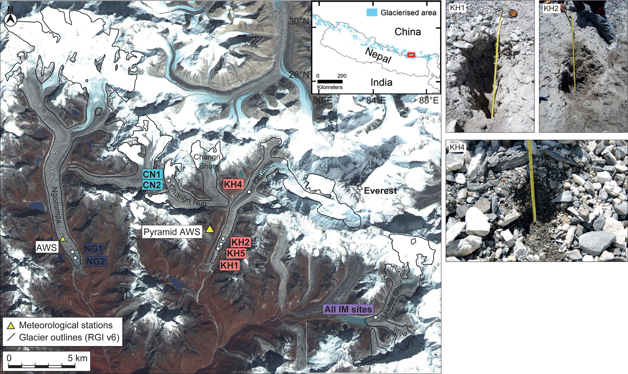
Fig. 1. Location map of the Everest region of Nepal showing sites where debris temperatures were measured on Ngozumpa, Khumbu, Changri Nup and Imja-Lhotse Shar Glaciers. Glacier outlines are taken from the Randolph Glacier Inventory (v6.0; RGI Consortium, 2017). Topographic imagery is from Landsat bands 7, 5 and 4 in 2015. Inset shows the location of the main figure. Photos show examples of the debris at sites KH1, KH2 and KH4.
2. Field sites
Our study targeted four glaciers in Sagarmatha National Park, Nepal, that discharge meltwater to the Dudh Kosi catchment. The first, Khumbu Glacier is a large debris-covered glacier 16 km long with an area of 19 km2 ranging from 4926 m to 7870 m above sea level (a.s.l.) with a median elevation of 5568 m a.s.l. (RGI Consortium, 2017). The debris layer is several metres thick near the terminus and generally thins up-glacier along the 9.8 km long ablation area to the base of the icefall (Nakawo and others, Reference Nakawo, Iwata, Watanabe and Yoshida1986). Thin, patchy debris is only found in a relatively narrow transition zone (Inoue and Yoshida, Reference Inoue and Yoshida1980). An estimate of debris thickness made in 1978 from observations of debris overlying ice cliffs was 0.5–2 m thick across the entire debris-covered surface and increased exponentially down-glacier to reach over 2 m thick near the terminus (n = 50) (Nakawo and others, Reference Nakawo, Iwata, Watanabe and Yoshida1986). Measurements made in 2014 by excavation of debris ranged up to 3.0 m with a mean value of 0.35 m (n = 64) (Soncini and others, Reference Soncini, Bocchiola, Confortola and Minora2016). Our measurements made by excavation of debris in 2014 estimated that 80% of the area between the terminus and 3.5 km up-glacier was covered with debris over 1 m thick (n = 143) with thinner (0.04–1.0 m) debris observed at the perimeter of supraglacial ponds or on the top of ice cliffs (Gibson and others, Reference Gibson2018).
Changri Nup Glacier is a former tributary of Khumbu Glacier that is now detached from both Khumbu Glacier and its own former debris-free tributary. Debris-covered Changri Nup Glacier is 4 km long with an area of 3 km2 ranging from 5240 m to ~6700 m a.s.l., with a 2.3 km long debris-covered tongue (Vincent and others, Reference Vincent2016). These glacier statistics are notably different from the description given as part of the combined Changri Nup–Changri Shar Glaciers by the RGI Consortium (2017).
Ngozumpa Glacier is the largest glacier in Nepal, nearly 20 km long with an area of 61 km2 ranging from 4702 m to 8181m a.s.l. with a median elevation of 5815 m a.s.l. (RGI Consortium, 2017). The lower 15 km of the glacier is covered in rock debris increasing in thickness to reach 1–3 m towards the terminus (Nicholson, Reference Nicholson2005). Mean debris thickness measured at two sites within 7 km of the terminus of Ngozumpa Glacier in 2001 was 1.25 ± 0.75 m (n = 218) (Nicholson and Benn, Reference Nicholson and Benn2013).
Imja-Lhotse Shar Glacier is a compound debris-covered glacier located 12 km southeast of Khumbu Glacier with an area of 14 km2 that refers to both the northwest-flowing Imja Glacier and southwest-flowing Lhotse Shar Glacier that converge and terminate into a proglacial lake, ranging from 5021 m to 7988 m a.s.l. with a median elevation of 5366 m a.s.l. (RGI Consortium, 2017). There is extensive debris cover below 5200 m a.s.l. on Imja Glacier and below 5400 m a.s.l. on Lhotse Shar Glacier. Mean debris thickness measured on part of Imja-Lhotse Shar Glacier in 2013 was 0.42 ± 0.29 m (n = 25) (Rounce and McKinney, Reference Rounce and McKinney2014).
The four glaciers are located adjacent to each other (Fig. 1) and their ablation areas are covered with extensive supraglacial debris layers with a similar range of thicknesses, composed of a similar mixture of clasts of leucogranite, sillimanite-grade gneiss and minor schist that range in size from boulders many metres in diameter to fine sand and silt (Benn and others, Reference Benn2012). We therefore do not expect to find differences in debris properties that are specific to individual glaciers and instead consider the dataset from the four glaciers as a whole.
3. Methods and data
3.1 Meteorological measurements
Meteorological measurements of air temperature, precipitation and relative humidity were made concurrent to debris temperature measurements to facilitate their interpretation (Fig. 2). Off-glacier air temperature was measured at an automatic weather station 5035 m a.s.l. at the Pyramid Observatory adjacent to Khumbu Glacier (Fig. 1), which is part of the SHARE Network operated by EV-K2-CNR. Off-glacier precipitation was measured using a Geonor T-200BM sensor that captures all precipitation phases and corrected for snow undercatch following World Meteorological Organisation recommendations (Sherpa and others, Reference Sherpa2017). On-glacier air temperature was measured at three sites on Khumbu Glacier through the 2014, 2015 and 2016 monsoon seasons (May–October) using thermistors mounted in naturally ventilated radiation shields 1 m above the glacier surface connected to Gemini Tiny Tag Plus2 TGP-4520 dataloggers with a stated accuracy of ±0.4°C at 0°C. Air temperature and relative humidity were measured on Changri Nup Glacier with an automatic weather station using a Vaisala HMP155A that was artificially ventilated during daytime using an Atmos aspirated radiation shield (reference: 43502). Air temperature was measured at four sites on Ngozumpa Glacier in 2002 using a Campbell 50Y thermistor with a stated accuracy of ±0.35°C mounted 1.5 m above the glacier surface and connected to a Campbell CR510 datalogger. Air temperature was not measured at Imja-Lhotse Shar Glacier.
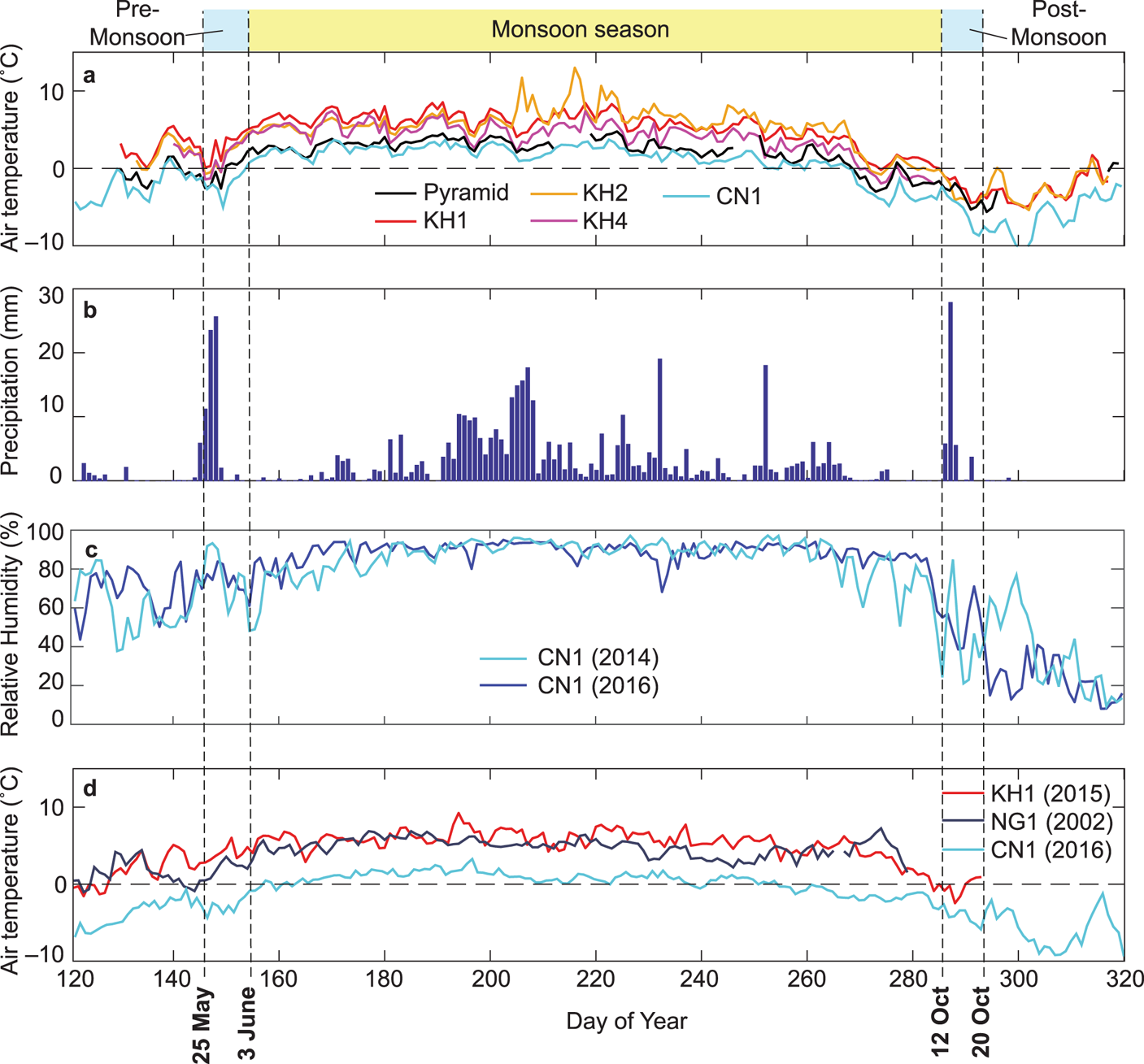
Fig. 2. Daily off-glacier and on-glacier meteorological data. (a) Mean daily air temperatures measured at Khumbu Glacier, Changri Nup Glacier and the Pyramid Observatory in 2014, (b) daily precipitation amount measured at the Pyramid Observatory in 2014 (as rain plus snow in water equivalent), (c) mean daily relative humidity measured at Changri Nup Glacier in 2014 and 2016, and (d) mean daily air temperatures measured at Khumbu Glacier in 2015, Ngozumpa Glacier in 2002 and Changri Nup Glacier in 2016.
3.2 Debris temperature measurements
We measured near-surface debris temperature (T s) and temperature through debris (T d) of varying thicknesses at 12 sites on four glaciers over several years. Temperature at the debris–ice interface (T i) was also measured at seven sites where excavation to the base of the debris layer was possible. The site locations are shown in Figure 1 and the data collection is summarised in Table 1. Data from Ngozumpa Glacier site NG1 and Imja-Lhotse Shar Glacier have been described, respectively, by Nicholson and Benn (Reference Nicholson and Benn2013) and Rounce and others (Reference Rounce, Quincey and McKinney2015), while the remaining data from Khumbu Glacier, Changri Nup Glacier and Ngozumpa Glacier site NG2 are reported for the first time here.
Table 1. Description of the debris temperature measurement sites on Khumbu, Changri Nup, Ngozumpa and Imja-Lhotse Shar Glaciers in the Everest region of Nepal
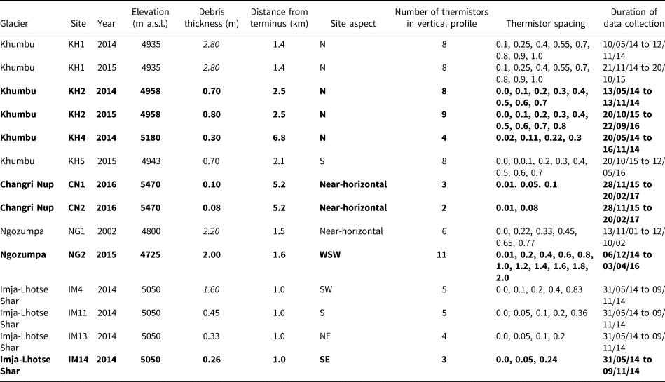
Debris thickness values in italics indicate where the debris layer was too thick to excavate to the debris–ice interface and values were estimated using the mean ablation season near-surface temperature and debris temperature gradient for the site. Sites highlighted in bold indicate those where measurements were made through the debris column to the debris–ice interface. Distance from the terminus is relative to that indicated by the RGI outlines (RGI Consortium, 2017).
Debris temperatures were measured at three sites on Khumbu Glacier (KH1, KH2 and KH4) through the 2014 monsoon season (May–October). Further data were collected at KH1 through winter 2014/2015, and at KH2 and KH5 through 2015/16. All sites were located on gently inclined slopes offset from the crests of topographic highs where debris was up to1 m thick. At KH1, KH2 and KH5, debris was dominated by light-coloured gneiss and leucogranite with minor schist fragments, whereas at KH4 debris contained gneiss and leucogranite but was generally darker and more angular due to a greater proportion of schist. The grain size of the debris ranged between coarse sand and decimetre-sized clasts and was generally finer than the bulk grain size of the whole debris layer as sites were chosen where sections could be excavated rather than where metre-scale boulders occupied the glacier surface. At each site, a vertical section was excavated, and thermistors were placed within the exposed section at measured intervals between the debris surface and the debris–ice interface. The excavated debris was then replaced as close to the original condition as possible. Temperature was sampled every 30 min. Thermistors measuring T s were shielded from incoming shortwave radiation by covering them with ~0.02 m of debris so that near-surface rather than surface temperature was measured, as the latter is highly dependent on incoming solar radiation (Gibson and others, Reference Gibson2018). All thermistors were connected to Gemini Tiny Tag Plus2 TGP-4520 dataloggers with a stated accuracy of ±0.4°C at 0°C.
Debris temperatures were measured at two sites on Changri Nup Glacier (CN1 and CN2) between November 2015 and February 2017. These data were measured every minute then averaged to give a 30 min time step using TCA PT100 with a stated accuracy of ±0.1°C. Data from these sites collected after 25 July 2016 are not used as both sites were covered with thick snow after this date indicated by the suppressed amplitude of T s.
Debris temperatures were measured at two sites on Ngozumpa Glacier (NG1 and NG2). Measurements at NG1 were made every 30 min from November 2001 to October 2002 using Gemini thermistors and Tinytag Plus TGP-0073 loggers with a stated accuracy of ±0.3°C at 0°C (Nicholson and Benn, Reference Nicholson and Benn2013). Measurements at NG2 were made at six-hourly intervals from December 2014 to April 2016 using a Geoprecision thermistor array with a stated accuracy of ±0.25°C.
Debris temperatures were measured at four sites on Imja-Lhotse Shar Glacier (IM4, IM11, IM13 and IM14) 1 km up-glacier from the lake-calving terminus at 5045–5055 m a.s.l. between May and November 2014. Measurements were made every 30 min using T&D Corporation TR-42 Thermo Recorder sensors with a stated accuracy of ±0.3°C (Rounce and others, Reference Rounce, Quincey and McKinney2015).
3.4 Effective thermal conductivity
Effective thermal conductivity (k) can be calculated if the effective thermal diffusivity, density, water content and specific heat capacity of the debris layer are known or estimated. Published values of k for supraglacial debris in Nepal and Europe are in the range 0.5–1.8 W m−1 K−1 (Table 2). These values are sensitive to debris water content; k can be up to three times greater for saturated debris than dry debris (Nicholson and Benn, Reference Nicholson and Benn2006). This method is dependent on T s and the differences in k between glaciers result from these measurements. Here, k was computed following the method of Conway and Rasmussen (Reference Conway and Rasmussen2000):

where h d is debris thickness and ρ c is the specific heat capacity of the debris. Debris temperatures were resampled to hourly increments, and apparent thermal diffusivity (k/ρ c) was taken as the linear fit between the derivative of temperature over time from hourly observations plotted against the second derivative of temperature with depth. Apparent thermal diffusivity was determined for the bulk layer using data from all levels of the debris cover simultaneously and each level individually. Visual inspection of these results allowed assessment of the presence of non-conductive processes (e.g. convective or latent heat exchange) within the debris profile, which are not represented in Eqn 1. On this basis, the site with the least evidence of non-conductive processes was selected from each glacier (KH1, NG1 and IM4) and thermal conductivity was computed from the bulk apparent thermal diffusivity for the summer months of July and August. This 2-month measurement period was deemed to be representative of the core ablation season and was used because these months show stable T d above 0°C, and is therefore not affected by seasonal temperature or water phase change that has been shown to affect k (Nicholson and Benn, Reference Nicholson and Benn2013). k was calculated from the apparent thermal diffusivity using the same value for ρ c (750 J kg−1 K–1 ± 10%) calculated from the rock density (2700 kg m−3) and effective porosity (0.33) used in previous studies in the region (Conway and Rasmussen, Reference Conway and Rasmussen2000; Nicholson and Benn, Reference Nicholson and Benn2013; Rounce and others, Reference Rounce, Quincey and McKinney2015). A conservative error on ρ c of 10% was assumed in line with previous studies (e.g. Conway and Rasmussen, Reference Conway and Rasmussen2000). Few data are available with which to quantify the uncertainties in the calculation of k using the method described here and we consider this value to be representative based on the range of possible values tested by Nicholson (Reference Nicholson2005). Uncertainties associated with the calculated apparent thermal diffusivity are included in the total uncertainty.
Table 2. Examples of bulk effective thermal conductivity values calculated for debris-covered glaciers in Nepal, Europe and Svalbard

Debris thickness values in italics indicate where the debris layer was too thick to excavate to the debris-ice interface and values were estimated using the mean ablation season near-surface temperature and debris temperature gradient for the site.
4. Results
4.1 Length of the 2014 summer monsoon season
We examined meteorological data collected from automatic weather stations at the Pyramid Observatory and on Changri Nup Glacier (Fig. 2) to determine the length of the monsoon season in 2014, for comparison with the length of the ablation season. The monsoon season in the upper Khumbu valley was characterised in 1994–2001 by cumulative precipitation amounts of between 382 mm and 442 mm (Bollasina and others, Reference Bollasina, Bertolani and Tartari2002). In 2014, the monsoon season started after a 9-day pre-monsoon transition period (25 May to 2 June) when we observed a storm that deposited decimetres of snow recorded as precipitation of up to 26.5 mm per day. Mean daily relative humidity (RH) reduced by ~40% during this period, then started to rise in tandem with air temperature from 3 June. Precipitation amounts measured at the Pyramid Observatory for June–September were 387 mm in 2013, 396 mm in 2014 and 332 mm in 2015 (Sherpa and others, Reference Sherpa2017). Precipitation, RH and T a remained high until a similar snowstorm occurred during mid-October, as a result of Cyclone Hudhud which reached Nepal on 14 October 2014 (Wang and others, Reference Wang, Gillies and Fosu2015; Shea and others Reference Shea2015b), causing an 8-day post-monsoon transition period when RH again fell by ~40% before the start of winter. The timing of these snowstorms was similar to the transitional periods (25 May–2 June and 12–19 October) recorded in previous years at the Pyramid Observatory (Bonasoni and others, Reference Bonasoni2010). The 131-day period between 3 June and 11 October that we describe as the monsoon season was defined by precipitation of up to 21.4 mm per day occurring on most days (122 of 131 days), giving a cumulative amount of 406 mm with a mean of 3.1 mm per day, while mean daily air temperature remained above 0°C and mean daily RH remained above 60%. The highest air temperatures occurring from mid-August until the last week of September when RH was above 80%.
4.2 Length of the ablation season from debris–ice interface temperatures
As we seek to investigate the duration of the ablation season, which is likely to extend beyond the core monsoon season, we start by using data from the six summer months (1 May to 31 October) to identify when ablation occurs. We define the ablation season as the days when the mean daily temperature at the debris–ice interface is within measurement uncertainty of 0°C. We identified the ablation season beneath supraglacial debris using T i for seven sites (KH2, KH4, KH5, CN1, CN2, NG2 and IM14; Table 1; Fig. 3). On average, the ablation season started in mid-April and ended in late October. Ablation occurred at the debris–ice interface for a continuous period of 141 days (23 May to 11 October; DOY 143–284) where debris was up to 0.1 m thick at CN1 and CN2 (Fig. 4). Ablation occurred for 160 days (approximately 15 May to 22 October; DOY 135–295) where debris was 0.3–0.7 m thick at KH2, KH4, KH5 and IM14. At NG2 where debris was 2.0 m thick, the ablation season appeared longer based on the period when T i was within uncertainty of 0°C (28 April to 4 December; DOY 118–338). However, these data were collected at six-hourly intervals and as such do not capture the diurnal T i signal. The debris temperature gradient (δT d/δh d) at the base of the debris layer at NG2 (Fig. 5) was zero between 28 April and 15 May indicating no heat flux to the ice surface and positive between 22 October and 4 December indicating heat flux away from the ice surface, confirming that the ablation season at NG2 was also 160 days (DOY 135–295).

Fig. 3. Summer debris temperatures (T d) measured during the 2002, 2014 and 2015. Daily mean T d isotherms for the debris layer during the monsoon season at all three glaciers for the site and year given in the figure. All debris thicknesses are plotted to the same scale and the colour scale for T d is the same in each case. A dashed line indicates where the profile reached the debris–ice interface. Where data are not aligned with the upper axis this indicates that the uppermost thermistor was not located at the debris surface. Note that measurements made at KH5 are not shown as due to collapse of these debris profile only an incomplete temperature time series was recorded, or at Changri Nup sites CN1 and CN2 as the debris profiles here were less than 0.1 m thick.

Fig. 4. The relationship between length of ablation season at the debris–ice interface and elevation, with colour shading showing debris thickness. Shaded bars show the estimated length of ablation season where the measurement period only captured part of the period represented by the filled circle.
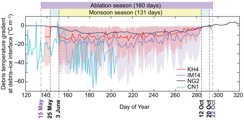
Fig. 5. Variability in the daily debris temperature gradient at the base of the debris layer at KH4, CN1, NG2 and IM14 where debris temperatures were measured to the debris–ice interface through the ablation season. The solid lines show the mean daily temperature gradient and the shaded areas show the diurnal range of minimum and maximum gradient for each site. Note that measurements at NG2 were made every 6 h compared to every 30 min at KH4 and IM14, and as a result appear smoother and have a narrower diurnal range. The diurnal range is not shown for CN1 as this varied from −314 to 97°C m–1 as a result of the thin debris (0.1 m) at this site; a similar trend was observed at CN2 where the debris layer was 0.08 m thick. Measurements for CN1 are not shown after 25 July 2016 (DOY 207) as after this date the debris surface was insulated by thick snow cover and these data were excluded from analysis.
Mean daily T i indicate that the May 2014 snowstorm interrupted the ablation season for 5 days at KH2 and 6 days at KH4 with warmer T i measured before and after this event. Despite warm daytime T a, surface snow insulated the glacier surface and subsurface and T s and T d remained below 0°C with no detectable diurnal signal for 5 days at KH2 during the May 2014 snowstorm and a suppressed diurnal signal for 7 days during the October 2014 snowstorm (Fig. 3). Similarly at Imja-Lhotse Shar Glacier, the surface was assumed to be snow-covered and ablation to be zero during 26 May–1 June and 13–20 October 2014 (Rounce and others, Reference Rounce, Quincey and McKinney2015). In May 2014, T s and T d indicate that snow lasted for 6 days at KH2 and 7 days at KH4, which is 220 m higher in elevation, suggesting that snow lay slightly longer on the upper ablation area of Khumbu Glacier.
4.3 Ablation season debris temperature gradients
Mean seasonal temperatures through the debris layer at each site were fitted with a linear regression to estimate the debris temperature gradient so that these can be compared between sites. Each vertical debris profile showed an approximately linear temperature gradient through the entire ablation season (Fig. 6a). A linear relationship gave a good fit to each profile, giving coefficient of determination (r 2) values >0.83 (Table 3). The debris temperature gradient exhibited a power-law relationship with debris thickness that became shallower with increasing debris thickness (r 2 = 0.96), giving ~−40°C m–1 where debris was up to 0.1 m thick, ~−20°C m–1 for debris between 0.1 and 0.5 m thick, and ~−4°C m–1 for debris >0.5 m thick (Fig. 7b; Table 3). T s varied between sites from 3.3 to 9.4°C for debris thicknesses of 0.08–2.8 m (Table 3), and also exhibited a power-law relationship with debris thickness (r 2 = 0.90) (Fig. 7a). Across our four study glaciers, sites with debris layers <0.5 m thick are found between 5050 m and 5470 m a.s.l. and have mean T s of 4.9°C. Sites with debris layers more than 0.5 m thick are found between 4725 m and 5050 m a.s.l. and have mean T s of 7.7°C. The difference in Ts of 2.8°C across a mean elevation difference of 250 m is not accounted for by warmer air temperatures at lower elevation. Debris thickness was estimated from T s for sites where it could not be measured directly by assuming that T i is 0°C during the ablation season and using the debris temperature gradient for each site to give debris thickness of 2.8 m at KH1, 2.2 m at NG1 and 1.6 m at IM4 (Table 3).
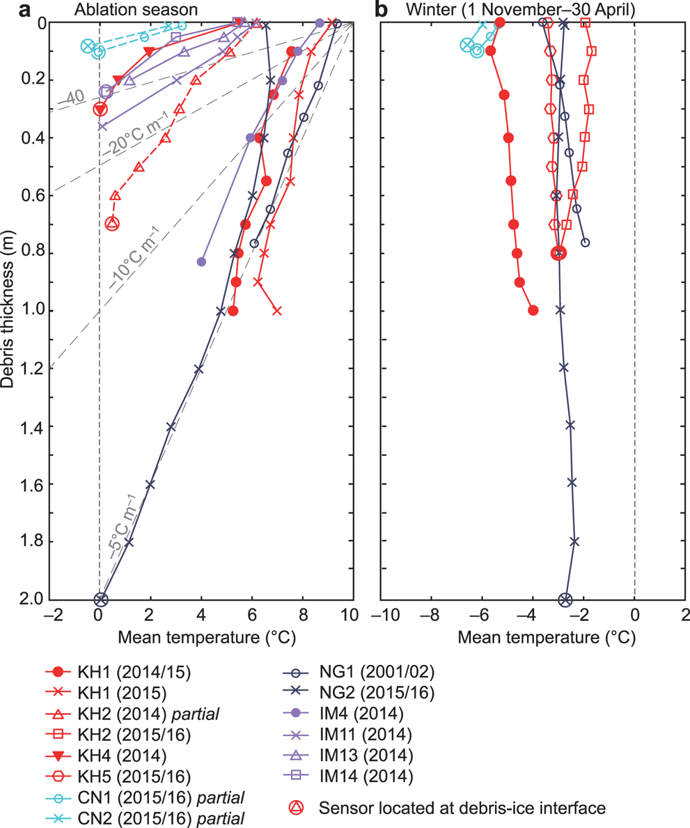
Fig. 6. Seasonal debris temperature profiles for Khumbu, Changri Nup, Ngozumpa and Imja-Lhotse Shar Glaciers for (a) the ablation season at the site and (b) winter (1 May to 30 April). Where the debris temperature profile reached the debris–ice interface this is indicated by a circle. The grey dashed lines indicate example debris temperature gradients with the values given alongside the line. The mean daily standard deviations of debris temperature are not shown; for summer these range from 2.3°C (CN2) to 4.4°C (IM13) and for winter from 3.2°C (KH5) to 6.7°C (CN1). Note that in (a), the data shown with dashed lines are partial time series; for KH2 ending on 30 June 2014 after which the sensors at the base of the debris layer migrated away from the debris–ice interface, and for CN1 and CN2 where the debris surface was covered with a thick layer of snow from 25 July 2016 onwards. Coefficients of determination (r 2) for the linear profile fits are given in Table 3.
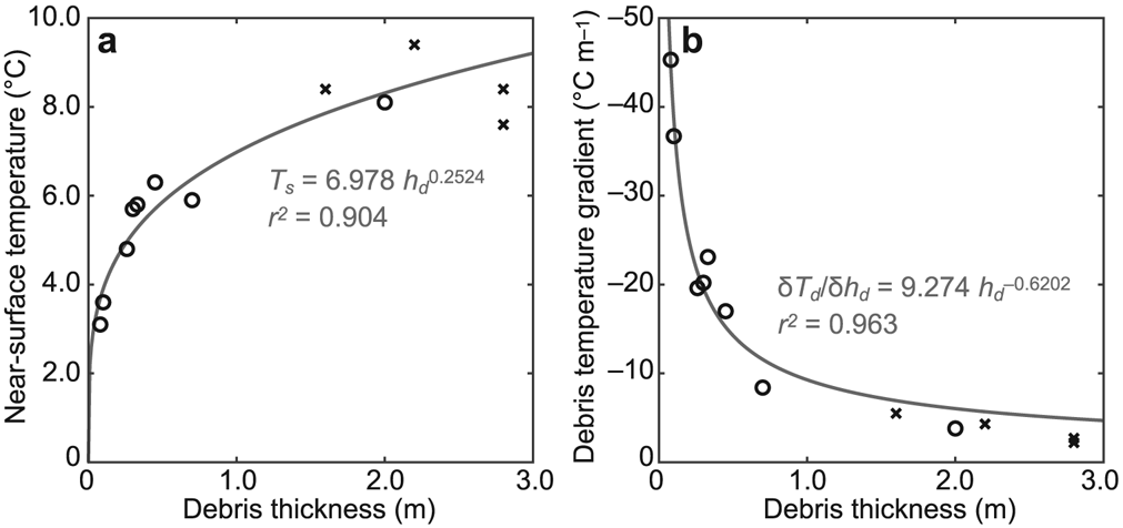
Fig. 7. Power-law relationships between debris thickness and near-surface temperature and debris temperature gradient for the ablation season, showing (a) debris thickness against near-surface temperature, and (b) debris thickness against debris temperature gradient. The sites where debris thickness to the debris–ice interface was observed are shown by circles and the sites where debris thickness was estimated are shown by crosses. KH1 (debris thickness = 2.8 m) is shown twice as measurements were made at this site in two separate time series across two different years. Grey lines show the power-laws fitted using only the data where debris thickness was observed (circles). If the entire dataset is used, then the fits are similar, yielding coefficients of determination (r 2) of 0.886 for debris thickness–near-surface temperature (a) and 0.973 for debris thickness–debris temperature gradient (b).
Table 3. Duration and characteristics of the ablation season beneath supraglacial debris
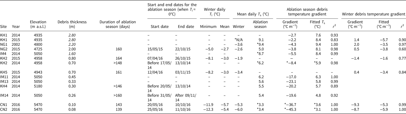
Near-surface temperatures (T s), debris–ice interface temperatures (T i), mean daily and seasonal summer and winter debris temperature gradients for sites sorted according to debris thickness on Khumbu, Changri Nup, Ngozumpa and Imja-Lhotse Shar Glaciers. Debris thickness values in italics indicate where the debris layer was too thick to excavate to the debris–ice interface and were estimated using the mean ablation season T s and the debris temperature gradient for the site. Asterisks (*) indicate partial data series: NG1 T s time series ends on 6 October 2002; IM4 T s time series starts on 31 May 2014; KH2 end of ablation season is indicated by sensor that migrated away from the debris–ice interface and is likely to be a minimum value; at CN1 and CN2 thick snow cover from 25 July 2016 suppressed T d and these data are excluded.
We examined in detail four profiles where measurements were made through the entire debris thickness to the debris–ice interface (KH4, CN1, IM14 and NG2; excluding CN2 where T d was only measured at one depth) to investigate diurnal variations in the debris temperature gradient during the ablation season. The standard deviation of T d for each profile decreased with debris thickness as the amplitude of the diurnal signal was suppressed at depth, giving values at the debris–ice interface of 0.66°C at KH4, 0.81°C at CN1, 0.19°C at NG2 and 0.06°C at IM14. Analysis of the debris temperature gradient at the debris–ice interface confirmed the duration of the ablation season estimated from T i values as 160 days at each of these sites apart from CN1 where the ablation season was 20 days shorter. The debris temperature gradient varied over time, with the change from positive to negative values at the debris–ice interface indicating the start of the ablation season when net heat flux was downwards towards the ice surface (Fig. 5). The range of values for the debris temperature gradient at the debris–ice interface varied between sites, with the greatest range of −314°C m–1 to 97°C m–1 observed at CN1 from the start of the ablation season to 25 July, after which period the data from this site were discarded due to insulation by overlying snow, which decreased the debris temperature gradient to less than −20°C m–1. At each of the other three sites, although the debris temperature gradient varied between days, values remained negative, indicating continuous ablation during the 160-day period (Fig. 5).
4.4 Winter debris temperature gradients
Winter was defined as the 6-month period (1 November to 30 April) when mean daily air temperatures were below 0°C and ablation did not occur. Mean winter T i recorded at five sites (KH2, KH5, CN1, CN2 and NG2) ranged from −5.7°C to −2.7°C (Table 3) and daily values were consistently below 0°C, indicating that sub-debris ice surfaces remained frozen at elevations above 4700 m a.s.l. between 1 November and 30 April each year. Winter T d remained below 0°C through the entire debris column at each site (Fig. 6b), although a few days with positive temperatures were recorded in the upper sections of the debris layers. A sudden jump to warmer T d was observed at KH2 and KH5 at the end of January, which may indicate when these sites were first exposed to direct solar radiation during the winter. Winter debris temperature gradients were close to vertical, giving ~−9.0°C m–1 at CN1 and CN2 where debris thickness was up to 0.1 m, and ranging from −1.4°C m–1 to 2.0°C m–1 for five sites with debris thickness greater than 0.7 m (Table 3).
4.5 Effective thermal conductivity
Estimating effective thermal conductivity (k) relies on assuming that the thermal properties of the debris are relatively constant in space. However, the hourly thermal profiles used to calculate k showed greater between-site variation than expected, likely as a result of non-conductive processes, rapidly changing temperatures, strong stratifications or some combination of these factors. Non-conductive processes or vertical stratification in debris processes were indicated by the large residuals around the best-fit line of the scatter plot of temperature derivatives used to estimate apparent thermal diffusivity from which effective conductivity was calculated. For each glacier, the site with the least evidence of non-conductive processes was used to calculate k, assuming that this single value is representative at the glacier scale; a realistic assumption if the debris lithology and moisture content are consistent. Calculated k was 0.98 ± 0.10 W m–1 K–1 for KH1, 1.43 ± 0.14 W m–1 K–1 for NG1 and 1.98 ± 0.20 W m–1 K–1 for IM4, each of these sites has a debris thickness greater than 1.6 m and T d measurements were only made in the upper part of the profiles to a maximum depth of 0.77–1.0 m (Table 1). These values are similar to those observed for other sites on these glaciers and for other debris-covered glaciers in Nepal and Europe (Table 2).
5. Discussion
5.1 Anomalies in our data collection
At five sites, only part of the air temperature, T i or T d time series could be used in our analyses, and these anomalies are summarised here and indicated in Table 3. At KH2 the T i measurement was >0°C after 30 June 2014 (Fig. 3) suggesting that the thermistor lost contact with the ice surface. Although thermistors were placed at the debris–ice interface at the start of the measurement period and the site remained intact, ablation of the underlying ice likely caused the thermistor to migrate with the base of the debris resulting in positive values where T i should have been measured. At CN1 and CN2, the debris surface was covered with a thick layer of snow from 25 July 2016 until the end of the ablation season, which insulated the debris surface and suppressed the flux of heat through the debris layer. At NG1, the T s time series ends on 6 October 2002 before the end of the T d time series, which continues for a further 6 days. At NG2, although the debris temperature gradient was similar to that measured through other thick debris layers during the ablation season, T s was ~3°C colder than predicted based on extrapolation of a linear debris temperature gradient to the debris surface. The shape of the T d profile indicates that T s could have been biased by an external factor such as greater exposure to cold air temperatures or snow collecting around the thermistor during the ablation season, particularly as these measurements were made every 6 h rather than every 30 min, and so may not have captured the full diurnal temperature range. A linear fit to the NG2 profile excluding the uppermost sensor gives a value for T s of 8.1°C rather than 5.0°C. During winter, T s is also warmer than expected by ~1°C, and likely biased by the same factor that affected ablation season measurements at this sensor. Collecting measurements of debris temperature and surface temperature across a glacier surface is challenging, particularly over seasonal time scales, as during the ablation season sensor migration and exposure of near-surface sensors can occur due to movement of the glacier surface, and consequently it can be difficult to assess the reliability of such measurements.
5.2 Uncertainty in the length of the ablation season
The length of the ablation season was similar for all sites apart from CN1 and CN2, suggesting that the duration of ablation decreased with debris thickness and site elevation (Fig. 4; Table 3). The duration of the ablation season was similar beneath a range of debris thickness from 0.26 m to 2.2 m, indicating that the duration of the sub-debris melt is controlled by atmospheric forcing rather than site-specific factors and remains fairly consistent across the wide area represented by our four study glaciers. At ten sites, the duration of sub-debris melt was 29 days longer than the monsoon season, as daily air temperatures and relative humidity begin to rise after the winter from April, when the amount of incoming solar radiation reaching the debris surface each day also increases. CN1 and CN2 were 400–500 m higher and had thinner debris covers than the other sites, and their ablation season was 20 days shorter. Supraglacial debris thickness and the length of the ablation season generally reduced with increasing site elevation (Fig. 4), and it is not clear which variable is more important in controlling the duration of sub-debris melt. Previous work on Satopanth Glacier in the Central Himalaya has demonstrated that debris thickness is more important than glacier elevation in controlling the magnitude of sub-debris melt (Shah and others, Reference Shah, Banerjee, Nainwal and Shankar2019). The shorter ablation season at higher elevation sites could be due to more effective heating over thinner debris layers (Steiner and Pellicciotti, Reference Steiner and Pellicciotti2016). We note that the 131-day length of the monsoon season that we define is in line with that from previous observations made at the Pyramid Observatory (Bollasina and others, Reference Bollasina, Bertolani and Tartari2002). However, if we define the monsoon season more strictly as the period where mean daily air temperatures remain positive, relative humidity remains above 90% and precipitation occurs on at least 2 of every 3 days, then the monsoon season could be between 3 and 4 weeks shorter, starting around the middle of June and ending at the end of September (Fig. 2).
We investigated if it were possible to identify the length of the ablation season from air temperature or surface temperature using the lag between when mean daily T i was within measurement uncertainty of 0°C, indicating the occurrence of ablation, and when mean daily air temperature or mean daily T s were >0°C. However, we do not have a complete time series of T i that captures both the start and end of the ablation season and has concurrent air temperature measurements. An initial assessment based on the available data from four sites showed that T s was warmer than 0°C for 6 days before the start of the ablation season at NG2. T s cooled below 0°C 22 days before the end of the ablation season at NG2, whereas at KH4 the end of the ablation season occurred on the same day that T s cooled below 0°C, which was 13 days after air temperature cooled below 0°C. At CN1, T s warmed above 0°C 23 days before the start of the ablation season, and earlier than the first positive mean daily air temperatures, which occurred 3 days after the onset of ablation. Mean daily air temperature dipped in subsequent days and did not remain consistently above 0°C until 9 days after the start of the ablation season. At CN2, T s warmed above 0°C on the same day as at CN1, which was 28 days before the start of the ablation season. Here the first positive mean daily air temperatures occurred 2 days before the onset of ablation. T s started to warm above 0°C before the start of the ablation season at both CN1 and CN2, and prior to this the debris surface also warmed above 0°C during a series of 1- to 3-day periods starting 47 days earlier. T i at both sites showed similar trends through the winter, but as T s started to warm T i remained higher at CN1 where the debris layer was 25% thicker, causing the onset of the ablation season 5 days earlier. The onset of ablation at the Changri Nup sites does not seem to have been driven by air temperature but instead followed T s, which is dependent on incoming solar radiation and turbulent fluxes (Steiner and others, Reference Steiner2018). The relatively small difference in debris thickness of 0.02 m between these sites appeared to result in an earlier onset of ablation where debris is thicker at CN1 but this couldbe affected by other site characteristics such as aspect or debris lithology.
5.3 Seasonal stability in the thermal properties of supraglacial debris
Ablation season and winter debris temperature gradients were all approximately linear, indicating that the thermal properties of the debris layer can be approximated by a constant value over seasonal time scales, and T s was shown to be a function of debris thickness, as observed by Nicholson and Benn (Reference Nicholson and Benn2013). If T s is known for the duration of the ablation season, then a linear value for the debris temperature gradient can be used to estimate debris thickness and sub-debris ablation. The consistency of seasonal debris temperature gradients between sites indicates that the material properties of the debris at each site are likely comparable, which is not unreasonable for neighbouring glaciers, but valuable to know in regard to applying thermal properties measured at a single or small number of sites to a whole glacier or number of glaciers. Furthermore, this raises the possibility of scaling the debris temperature gradient, which drives the delivery of energy for melting the underlying ice, as a function of debris thickness to calculate sub-debris melt from T s. Given the limitations of our dataset, we refrain from proposing the form of such a relationship, but note that on the basis of our data collection, it appears reasonable to apply such an approach at a catchment or even regional scale, and for our data, the relationship appears most likely to be a power function (Fig. 7b). Including more data or applying an energy-balance model to a range of debris thicknesses, such as that presented by Collier and others (Reference Collier2014), would be useful in establishing the forms of these relationships to allow the estimation of regional ablation beneath supraglacial debris from surface temperature, as this variable can be readily derived from satellite observations. That a predictable relationship between debris thickness and temperature exists for glaciers subject to the extreme seasonal variations in air temperature and precipitation amount represented by the Indian summer monsoon suggests that similar relationships are likely to hold for debris-covered glaciers elsewhere.
The timescale over which T s could be used to estimate debris thickness and sub-debris melt is a key consideration. Our analysis of the variability of the debris temperature gradient at the debris–ice interface demonstrated that there is some diurnal variability in the debris temperature gradient from the mean seasonal value, particularly at the start and end of the monsoon season. Informed by our analyses of effective thermal conductivity (k) for these glaciers, we expect that the core monsoon months of July and August represent the period when the debris layer is most thermally stable, and therefore are likely to most reliably reflect the seasonal trend. Based on the similarities between the sites in terms of climate, elevation, debris lithology and grain size, we would expect k values to be similar for each site and glacier over the same period of time. The variation in the values of k between sites indicate that non-conductive processes, rapidly changing temperatures, strong stratifications or some combination of these factors affect the thermal properties of the debris layer, particularly during periods of rapidly varying atmospheric conditions. We note that Rounce and others (Reference Rounce, Quincey and McKinney2015) found a much lower value for k at IM13 compared to the value we calculated, because their k values were calculated over a longer period (2 June to 12 October 2014) than that used here (1 July to 31 August). The difference between our results and those of Rounce and others (Reference Rounce, Quincey and McKinney2015) indicates that the apparent thermal diffusivity of the debris varies substantially during the ablation season, which could, for example, be due to phase changes during the monsoon season and changes in the water content of the debris layer over short distances.
Winter debris temperature gradients are typically invariant with depth and indicative of insulation of the debris surface by persistent snow cover. Negative values for the debris temperature gradient at KH1 in winter 2014/15 and at NG1 in winter 2001/02 occurred when the surface was snow free and the debris layer and underlying glacier surface could gradually lose heat to the cold winter atmosphere in the absence of the insulating snow layer. The winter debris temperature profiles were close to vertical, implying that T s gives a good estimate of temperature throughout the debris layer in winter, which, combined with the debris thickness, can be used to quantify the cold content that must be removed before ablation can begin. This observation could be used to provide a first crude estimate of the minimum delay in ablation onset arising from the need to heat the overlying debris layer at the start of the ablation season.
6. Conclusions
Supraglacial debris modifies the impact of atmospheric conditions on glacier mass balance and should be accounted for in calculating the response of debris-covered glaciers to climate change. However, the impact of summer monsoon meteorology complicates calculations of the duration and magnitude of ablation from debris-covered glaciers in the Himalaya and is poorly understood, as the majority of measurements are made over short periods. We measured temperatures through supraglacial debris during several monsoon seasons at 12 sites on four glaciers in the Everest region of Nepal, for which debris thickness ranged from 0.08 to 2.8 m and elevation ranged from 4725 m to 5470 m above sea level. Our results demonstrate that across this range of debris thicknesses, the length of the ablation season beneath supraglacial debris thicker than 0.1 m is ~160 days; at least a month longer than the monsoon season. Ablation at the debris–ice interface, indicated by temperatures rising from winter values to 0°C, occurs from approximately 15 May to 22 October each year, and can be interrupted for up to 10 days if a heavy snowfall occurs. During winter (1 November and 30 April), mean temperatures at the debris-ice interface were ~−4°C and debris temperature–thickness gradients were close to vertical, indicative of persistent snow cover and that the debris layer was thermally stable.
Although the transfer of heat through supraglacial debris was seen to vary through the ablation season in the reflection of meteorological events such as storms, debris temperature gradients calculated for the entire ablation season were approximately linear, giving values between −40°C m−1 and −4°C m−1 (r 2 > 0.83) across a range of debris thicknesses from 0.1 m to 2.8 m. The debris temperature gradient steepened by an order of magnitude as debris thickness increased from 0.1 to 1.0 m. Effective thermal conductivity, calculated during the core monsoon months (July–August) for three sites with debris thicknesses greater than 1.6 m ranged from 0.98 ± 0.1 W m–1 K–1 to 1.98 ± 0.2 W m–1 K–1, similar to values calculated for debris-covered glaciers elsewhere in Nepal and Europe. Mean ablation season debris near-surface temperature had a power-law relationship with debris thickness, meaning that this relationship can be used to predict debris thickness from surface temperature measurements. Our results quantify the thermal properties of supraglacial debris through the ablation season, demonstrating that mean seasonal values are representative of high-elevation monsoon-influenced debris layers in general. These relationships can therefore be used to improve calculations of the impact of supraglacial debris on the mass balance of debris-covered glaciers elsewhere in the monsoon-influenced Himalaya, and to improve projections of the response of these glaciers to climate change.
Acknowledgements
Fieldwork at Khumbu Glacier was supported by Royal Society Research Grant RG120393 to A. Rowan and D. Quincey and a grant from the Mount Everest Foundation to A. Rowan. L. Nicholson was supported by Austrian Science Fund (Project numbers V309 and P28521). Yves Lejeune is thanked for processing precipitation data, and Pierre Chevallier for processing air temperature data collected at the Pyramid Observatory. The meteorological dataset contained within this study was collected within the framework of the Ev-K2-CNR Project in collaboration with the Nepal Academy of Science and Technology as foreseen by the Memorandum of Understanding between Nepal and Italy, and thanks to contributions from the Italian National Research Council, the Italian Ministry of Education, University and Research and the Italian Ministry of Foreign Affairs. We thank Himalayan Research Expeditions and Summit Trekking for support and guiding in the field. We thank the Scientific Editor, Dan Shugar, and an anonymous reviewer for their helpful comments that improved the presentation of this work.
Author contributions
AR, LN and DQ designed the original study. AR, DQ, MG, TI-F and SW carried out fieldwork at Khumbu Glacier in 2014, 2015 and 2016. LN collected data at Ngozumpa Glacier in 2001–2002. ST collected data at Ngozumpa Glacier in 2014–2016. DR collected data at Imja-Lhotse Shar Glacier in 2014. PW collected data from Changri Nup Glacier in 2016 and provided meteorological data from the Pyramid Observatory. All authors contributed to the discussion of the results and writing the manuscript.
Data availability
As the availability of debris temperature data is limited, it is of value to share these data publicly, and to that end we share all our data and invite other researchers with similar data to add to this database so that the ideas proposed in this paper can be explored more comprehensively. These datasets form a contribution to the International Association of Cryospheric Sciences' Working Group on Debris-Covered Glaciers. Debris thickness measurements from Khumbu Glacier; http://doi.org/10.5281/zenodo.3775571. Debris temperature data by glacier: Khumbu Glacier; https://doi.pangaea.de/10.1594/PANGAEA.883071. Changri Nup Glacier; http://doi.org/10.5281/zenodo.3048780. Ngozumpa Glacier, NG1; http://doi.org/10.5281/zenodo.3935687. Ngozumpa Glacier, NG2; http://doi.org/10.5281/zenodo.3935685. Imja-Lhotse Shar Glacier; http://doi.org/10.5281/zenodo.3906947.


 Open access