


1. Introduction
Ocean waves have been studied extensively by scientists and engineers. The distribution of wave heights given a stationary background sea state is of obvious interest. Particularly noteworthy are situations where large waves occur more frequently than would be expected in a linear model (Onorato et al. Reference Onorato, Residori, Bortolozzo, Montina and Arecchi2013; Adcock & Taylor Reference Adcock and Taylor2014; Trulsen Reference Trulsen2018). One mechanism that can cause this is where waves pass over a step, or steep slope, in the seabed. In a linear model with normally distributed random components, the free surface of the waves is expected to have a kurtosis of 3. Values of kurtosis as large as 3.6 have been observed in both numerical and experimental studies of waves at the top of slopes, meaning that a varying bathymetry can cause an increase in the size of large waves (Sergeeva, Pelinovsky & Talipova Reference Sergeeva, Pelinovsky and Talipova2011; Trulsen, Zeng & Gramstad Reference Trulsen, Zeng and Gramstad2012; Gramstad et al. Reference Gramstad, Zeng, Trulsen and Pedersen2013; Kashima, Hirayama & Mori Reference Kashima, Hirayama and Mori2014; Ma, Dong & Ma Reference Ma, Dong and Ma2014; Viotti & Dias Reference Viotti and Dias2014; Ducrozet & Gouin Reference Ducrozet and Gouin2017; Bolles, Speer & Moore Reference Bolles, Speer and Moore2019; Majda, Moore & Qi Reference Majda, Moore and Qi2019; Zhang et al. Reference Zhang, Benoit, Kimmoun, Chabchoub and Hsu2019; Trulsen et al. Reference Trulsen, Raustøl, Jorde and Rye2020; Zheng et al. Reference Zheng, Lin, Li, Adcock, Li and van den Bremer2020).
A number of attempts have been made to explain this phenomenon over the last decade. A review by Trulsen (Reference Trulsen2018) concludes that the transition over slopes can be a possible mechanism triggering non-equilibrium wave dynamics. A figure summarising experimental and numerical studies of this is given in Trulsen et al. (Reference Trulsen, Raustøl, Jorde and Rye2020). Our figure 1 extends this figure by adding additional studies as well as whether a peak in kurtosis is observed or predicted. Wave components at second order in wave steepness are found to be important (Gramstad et al. Reference Gramstad, Zeng, Trulsen and Pedersen2013; Viotti & Dias Reference Viotti and Dias2014; Zhang et al. Reference Zhang, Benoit, Kimmoun, Chabchoub and Hsu2019; Zheng et al. Reference Zheng, Lin, Li, Adcock, Li and van den Bremer2020). Two non-dimensional parameters are believed to play a key role in the problem (Li et al. Reference Li, Zheng, Adcock, Lin and van den Bremer2021; Trulsen et al. Reference Trulsen, Raustøl, Jorde and Rye2020). Specifically, these parameters are  $k_0h_d$ and
  $h_s/h_d$, composed of three characteristic lengths: the characteristic wavelength
  $\lambda _0=2{\rm \pi} /k_0$ (with
  $k_0$ the wavenumber) and the two water depths
  $h_d$ and
  $h_s$ on the deeper and shallower side, respectively.

Figure 1. Summary of studies of wave statistics affected by changes in bathymetry. The dimensionless group velocity  $c_g\omega /g$ (where
  $c_g$ denotes the group velocity,
  $\omega$ the wave frequency and
  $g$ the gravitational acceleration) based on the linear dispersion relationship is plotted (the red solid curve) as a function of dimensionless water depth
  $kh$ (where
  $h$ denotes water depth and
  $k$ is the wavenumber). The symbol ␣ denotes the two ends of water depths examined in the listed studies, from the depth on the shallower side
  $kh_s$ to the deeper side
  $kh_d$. The parameters in parentheses respectively denote
  $kh_s$,
  $kh_d$, the slope gradient, the method used (where FNPFS denotes fully nonlinear potential flow solver and NLS the nonlinear Schrödinger equation) and whether a local peak is found at the top of the depth transition (Y/N).
Since the 1960s there have been extensive studies of waves over a varying bathymetry that focus on other aspects. We review only those experimental studies most relevant to this paper. Seminally, Beji & Battjes (Reference Beji and Battjes1993) and Grue (Reference Grue1992) have examined changes to spectral shape due to the amplification of bound harmonics in response to varying bathymetry. As the first to systematically examine the role of depth transitions in enhancing the probability of abnormally large waves, Trulsen et al. (Reference Trulsen, Raustøl, Jorde and Rye2020) found that there can be a local maximum of the kurtosis and skewness of the surface elevation close to the shallower side of a ( $1\,{:}\,20$) underwater slope. Similar experiments were conducted and analysed by Zhang et al. (Reference Zhang, Benoit, Kimmoun, Chabchoub and Hsu2019). The sudden peak in kurtosis and skewness has also been observed in the laboratory when waves propagate over a step (Bolles et al. Reference Bolles, Speer and Moore2019) and on top of a shoal (Trulsen et al. Reference Trulsen, Raustøl, Jorde and Rye2020). In addition, Monsalve Gutiérrez (Reference Monsalve Gutiérrez2017) observed free superharmonic monochromatic waves at second order for weakly nonlinear regular waves over a step.
This paper presents an experimental study which aims to validate and explore the limitations of the second-order theory (in steepness) for narrow-banded surface gravity wavepackets experiencing a sudden depth transition derived in a companion paper (Li et al. Reference Li, Zheng, Adcock, Lin and van den Bremer2021). Different from all previous experimental studies, which have examined random or regular waves, we employ deterministic wave groups, which allow us to cleanly examine the physical mechanism at work. This study considers vertical steps as well as  $1\,{:}\,1$ and
  $1\,{:}\,3$ slopes and investigates a range of wave parameters and water depths.
This paper is laid out as follows. The theoretical framework employed is briefly reviewed in § 2, where the focus is on the application of the theory rather than the derivation, which is given in Li et al. (Reference Li, Zheng, Adcock, Lin and van den Bremer2021). The experimental matrix and set-up are detailed in § 3. Section 4 analyses the experimental results and compares with the theoretical model of Li et al. (Reference Li, Zheng, Adcock, Lin and van den Bremer2021). Conclusions are drawn in § 5.
2. Review of the theoretical model of Li et al. (2021)
Before introducing our experiments, we briefly review the theoretical model in the companion paper (Li et al. Reference Li, Zheng, Adcock, Lin and van den Bremer2021). This theoretical model (i) is based on potential flow theory neglecting surface tension, (ii) is correct to second order in wave steepness  $k_0A$, where
  $k_0$ and
  $A$ are the carrier wavenumber and amplitude, (iii) is valid for wavepackets of narrow bandwidth and (iv) assumes that the forcing of second-order terms by first-order evanescent waves near the depth transition is negligible. Finally, for the subharmonic bound and free waves at second order, we employ the additional assumption that the packet is long relative to the water depth (see § 2.6.3 in Li et al. Reference Li, Zheng, Adcock, Lin and van den Bremer2021).
2.1. Governing equations and boundary conditions
We consider weakly nonlinear unidirectional waves propagating over an abrupt change of depth. The abrupt depth change is modelled by a vertical wall, meaning that the water depth changes from a constant  $h_d$ to a constant
  $h_s$ at
  $x =0$, with
  $x$ denoting the horizontal coordinate. This is illustrated in figure 2. It is assumed that
  $h_d\geq h_s$ and that the water depth is intermediate (
 $kh={O}(1)$) on both sides of the step. Extremely shallow water is not considered. The system can be described as a boundary value problem:
 \begin{gather} \nabla^2 \varPhi = 0 \quad \text{for}\ -h(x) < z <0, \end{gather}
 \begin{gather}\dfrac{\text{D}}{\text{D}t} (z-\zeta) = 0,\quad g\zeta+\frac{\partial \varPhi}{\partial t} + \frac{1}{2} \left(\boldsymbol{\nabla}\varPhi \right)^2= 0 \quad \text{for}\ z= \zeta(x,t), \end{gather}
 \begin{gather}\frac{\partial \varPhi}{\partial z} = 0\quad \text{for}\ z={-}h(x) , \end{gather}
 \begin{gather}\left[\varPhi\right]_{x\to 0^-} = \left[\varPhi\right]_{x\to 0^+},\quad \left[\frac{\partial \varPhi}{\partial x}\right]_{x\to 0^-} = \left[\frac{\partial \varPhi}{\partial x}\right]_{x\to 0^+}\quad\text{for}\ -h_s < z < 0, \end{gather}
 \begin{gather}\left[\frac{\partial \varPhi}{\partial x}\right]_{x\to 0} = 0\quad\text{for}\ -h_d < z < {-}h_s, \end{gather}
in which  $\varPhi (x,z,t)$ is the velocity potential,
  $\zeta (x,t)$ is the surface elevation and
  $g$ is the gravitational acceleration.
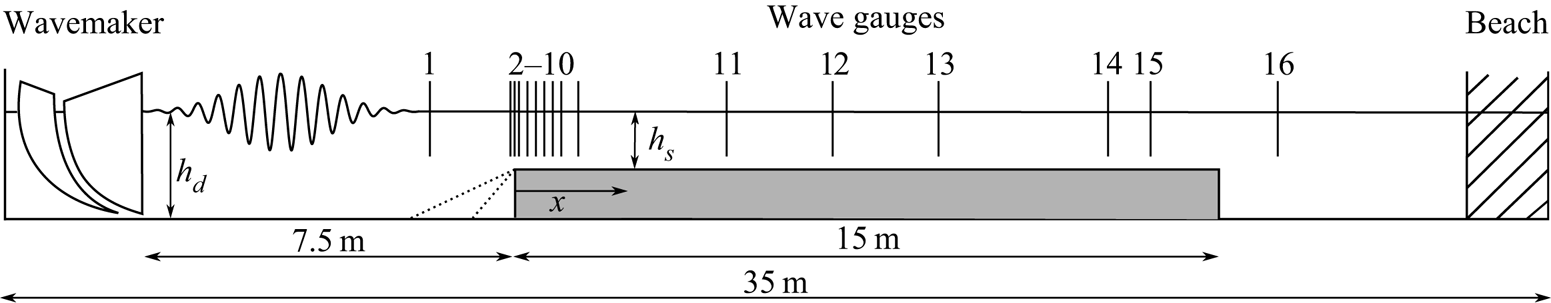
Figure 2. Diagram of test set-up including gauge, step, beach and wavemaker positions. Dashed lines denote the locations of the slopes, when installed. The horizontal positions of the gauges are listed in table 1.
2.2. Overall structure of the solutions
In Li et al. (Reference Li, Zheng, Adcock, Lin and van den Bremer2021), a perturbation expansion in the dimensionless wave steepness  $\epsilon$ and a multiple-scales expansion in the bandwidth parameter
  $\delta$ lead to approximate solutions of the boundary value problem (2.1). The solutions are expressed as functions of an incident wavepacket that is assumed known. Specifically,
 \begin{equation} \zeta= \zeta_{I} + \zeta_R +\zeta_{Ed} \quad \text{for}\ x<0,\quad \zeta= \zeta_{T} + \zeta_{Es} \quad \text{for}\ x>0, \end{equation}
where the subscripts  $I$,
$I$,  $R$,
$R$,  $T$ and
  $E$ denote the incident, reflected, transmitted and evanescent waves, respectively, and
  $d$ and
  $s$ denote the deeper and shallower sides. Up to the second order in steepness
  $\epsilon$, the free surface can be expressed as
 \begin{gather} \zeta_I(x,t) = \epsilon \zeta^{(11,0)}_I + \epsilon^2 [\zeta^{(22,0)}_{I,b}+\delta \zeta^{(20,1)}_{I,b}], \end{gather}
 \begin{gather}\zeta_R(x,z,t) = \epsilon \zeta^{(11,0)}_R + \epsilon^2 [\zeta^{(22,0)}_{R,b} + \zeta^{(22,0)}_{R,f}+ \delta(\zeta^{(20,1)}_{R,b} + \zeta^{(20,1)}_{R,f})] , \end{gather}
 \begin{gather}\zeta_{Ed}(x,t) = \epsilon \underbrace{\sum _{n=1}^{N\to \infty}\zeta^{(11,0)}_{En}}_{\zeta^{(11,0)}_{Ed}} + \epsilon^2\left[\underbrace{\sum _{n=1}^{N\to \infty} \zeta^{(22,0)}_{En}}_{\zeta^{(22,0)}_{Ed}}+\delta \underbrace{\sum _{n=1}^{N\to \infty} \zeta^{(20,1)}_{En}}_{\zeta^{(20,1)}_{Ed}}\right], \end{gather}
 \begin{gather}\zeta_T(x,t) = \epsilon \zeta^{(11,0)}_{T} + \epsilon^2[\zeta^{(22,0)}_{T,b} + \zeta^{(22,0)}_{T,f}+\delta(\zeta^{(20,1)}_{T,b} + \zeta^{(20,1)}_{T,f})], \end{gather}
 \begin{gather}\zeta_{Es}(x,t) = \epsilon\underbrace{\sum _{m=1}^{M\to \infty} \zeta^{(11,0)}_{Em}}_{\zeta^{(11,0)}_{Es}} + \epsilon^2 \left[\underbrace{\sum_{m=1}^{M\to \infty} \zeta^{(22,0)}_{Em}}_{\zeta^{(22,0)}_{Es}} +\delta\underbrace{\sum_{m=1}^{M\to \infty} \zeta^{(20,1)}_{Em}}_{\zeta^{(20,1)}_{Es}}\right], \end{gather}
where the superscripts  $(iq,j)$ denote the terms of
  ${O}(\epsilon ^i\delta ^j)$ that are proportional to the harmonics
  $\exp (\mathrm {i} q\psi _0)$, with
  $q=0$ corresponding to the subharmonic or ‘mean’ and
  $q=2$ to the superharmonic. The subscripts
  $b$ and
  $f$ denote the second-order bound and free wavepackets, respectively.
In (2.3), we have only given those terms that we might expect to observe in our experiments (see Li et al. (Reference Li, Zheng, Adcock, Lin and van den Bremer2021) for full details). At first order in wave steepness, an incident wavepacket is reflected ( $\varPhi ^{(11,0)}_R$) and transmitted (
 $\varPhi ^{(11,0)}_T$), complemented by the generation of evanescent waves (
 $\varPhi ^{(11,0)}_{Ed}$ on the deeper side and
  $\varPhi ^{(11,0)}_{Es}$ on the shallower side) near the step (cf. Massel Reference Massel1983). Both bound and free wavepackets can be distinguished at second order. First, bound waves are generated by combinations of linear waves, also arising in the absence of a step (cf. recent experiments by Calvert et al. (Reference Calvert, Whittaker, Raby, Taylor, Borthwick and van den Bremer2019)) and propagating together with the main (first-order) wavepacket. When the bound waves experience the depth transition, free waves are released in both directions. Free waves satisfy the linear dispersion relation and, hence, propagate independently. It is these free and bound second-order wavepackets that this paper examines experimentally.
3. Experimental methodology
3.1. Set-up, wave generation and data acquisition
We carried out experiments in the 35 m flume in the COAST (Coastal, Ocean and Sediment Transport) Laboratory at the University of Plymouth, UK. A schematic of the experiments is given in figure 2. The flume has a width of 0.6 m. It was filled to a depth  $h_d$, and a false floor of a height of
  $h_{{step}} = 0.35$ m was installed from 7.5 to 22.5 m away from the wavemaker. Hence, the water depth on the shallower side is
 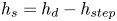 $h_s = h_d -h_{{step}}$ and depends on the deeper water depth
  $h_d$, which is varied in the experiments whilst keeping
  $h_{{step}}$ constant. In our experiments, we set
  $h_d$ to be 0.55 and 0.75 m.
We used a double-element piston-type wavemaker to generate a focused wave group with a narrow-banded Gaussian spectrum that linearly focuses to a Gaussian packet in space:
 \begin{equation} A_I(x,t) = A_0 \exp\left(-\frac{(x -x_{f} - c_{g0} (t-t_{f}))^2}{2\sigma^2} \right), \end{equation}
in which  $A_0$ is the focused wave amplitude for a uniform depth
  $h_d$ at a measurement zone located at
  $x_{f} = 1.0$ m (i.e.
  $8.5$ m from the resting position of the wavemaker) and at
  $t_{f} = 32$ s,
  $c_{g0}$ is the group velocity of the carrier wave on the deeper side and
  $\sigma$ is the characteristic envelope length that leads to
  $\delta = 1/(k_0\sigma )$. We note that the focused amplitude
  $A_s$ on the shallower side differs from the input
  $A_0$ by a factor of
  $|T_0|$, where
  $T_0$ denotes the transmitted coefficient for the linear carrier wave, i.e.
  $A_s=|T_0|A_0$. A total of 16 resistance-type wave gauges provided
  $128$ Hz free-surface elevation measurements at different locations depicted in figure 2 and defined in table 1. The measured free-surface signals, not the input signal, provided the parameters used to predict the theoretical surface elevation for each experiment.
Table 1. Horizontal positions of the gauges relative to the top of the depth transition ( $x=0$), as indicated in figure 2.

The wave paddles are controlled by a first-order signal, and hence both super- and subharmonic error waves (Schäffer Reference Schäffer1996) are expected to be generated, which have to be taken into account when analysing the experiments. After propagating through the measurement zone, the dispersed wavepackets were absorbed by mesh-filled wedges within an absorption zone located at the downstream end of the wave flume.
3.2. Experimental matrix
The main set of experiments are outlined in table 2. These consist of steps with two depth ratios  ${h_s}/{h_d}$ and a range of different peak frequencies
  $f_0$ (or
  $\omega _0$) for each depth. In addition, for
  $h_d = 0.55$ m, two sloped seabed structures with
  $1\,{:}\,1$ and
  $1\,{:}\,3$ slopes were examined with different frequencies
  $f_0$. The wave frequencies were chosen to guarantee that the depths on both sides of the abrupt depth transition are intermediate. The different frequencies and depth ratios were chosen to examine the effects of both the depth ratio
  $h_s/h_d$ and wave frequencies. The wave steepness
  $\epsilon =k_0A_0$ and bandwidth
  $\delta = 1/(k_0\sigma )$ were carefully selected and tested such that second-order effects are measurable but small enough that higher-order effects (i.e.
  ${O}(\delta ^2\epsilon ,\epsilon ^3)$ due to linear and nonlinear dispersion, respectively) do not play a significant role. The envelope length is long compared to the carrier wavelength and, thus, the narrow-banded wavepacket approximation is valid. The cases that were repeated three times are marked with an asterisk in table 2. Estimates of measurement errors are presented in appendix B, including an examination of repeatability in appendix B.2.
Table 2. Parameters of the main set of experiments. In the table,  $\epsilon = k_0A_0$ and
  $\delta = {1}/{(k_0\sigma )}$. Sets A and B are for steps with
  $h_d= 0.5$ and
  $0.75$ m, respectively; sets C and D are for slopes of
  $1\,{:}\,1$ and
  $1\,{:}\,3$, respectively. Cases with an asterisk have been repeated at least three times.

4. Results and discussion
This section discusses the experimental results, comparing with theoretical predictions using the model and solutions presented in the companion paper (Li et al. Reference Li, Zheng, Adcock, Lin and van den Bremer2021). The new physical mechanism, as evident in the measured data, is presented in § 4.1 and its consequences for skewness in § 4.2. The role of the two most relevant non-dimensional parameters, the carrier wavelength relative to the water depth  $k_0h_d$ and the depth ratio
  $h_s/h_d$, is examined in § 4.3 in a quantitative comparison with theory focusing on maximum surface elevation. Results for the two slopes are compared with results for the step in § 4.4.
4.1. Generation of free waves and local behaviour
In order to examine the sub- and superharmonic content of the time-domain measurements of the surface elevation at different locations, we separate the signals using frequency-domain filtering, which is described in detail in appendix A. Effectively, this leads to the separation of the wave harmonics that arise at different orders in  $\epsilon$ and include the (first-order) first harmonics
  $\zeta ^{(1)}$, the (second-order) subharmonics
  $\zeta ^{(20,1)}$ and superharmonics
  $\zeta ^{(22,0)}$.
To illustrate the new physical mechanism, we examine in detail case A5 in figures 3, 4, 5 and 6. Three additional cases, which illustrate qualitatively similar behaviour, are presented in appendix C. The results from both the theoretical model in Li et al. (Reference Li, Zheng, Adcock, Lin and van den Bremer2021) and the experiments are shown. The surface elevations in figures 4 and 13 are scaled by the measured linear peak amplitude  $A_s=|T_0|A_0$ at gauge 9 on the shallower side. We note that, in the experiments, the linear wavepackets did not focus exactly at any of the gauges. Amplitude
  $A_s$ was thus calculated from the spectra of linear waves at gauge 9 where linear packets were close to focus.

Figure 3. Energy spectra of surface elevation as a function of frequency at different gauge positions for cases A5, A2, B1 and B2. (a) Measured data at gauges 1 ( $x=-1.99$ m), 9 (
 $x=1.10$ m) and 14 (
 $x=14.0$ m). (b) Theoretical results versus the measured data at gauge 9. In the figure,
  $f_0$ is the carrier wave frequency.

Figure 4. Measured and theoretically predicted surface elevation separated out by harmonic and compared to theory for case A5. All surface elevations are scaled by the linear peak amplitude  $A_s =|T_0|A_0$ measured at gauge 9. The position (a) before the step, (b) near the step on the shallower side and (c) far downstream of the step.

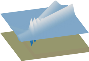
Figure 5. Spatio-temporal evolution of superharmonic wavepackets associated with case A5.

Figure 6. Spatio-temporal evolution of subharmonic wavepackets associated with case A5.
The energy spectra for four cases are shown in figure 3, which shows the experimental data at three gauges and the comparisons of the wave energy between experiments and theory at gauge 9. It can be clearly observed in figure 3(a) that energy near  $3\times f_0$ is three to four orders of magnitude smaller than the energy near
  $1\times f_0$, as expected for the small
  $\epsilon$ in the experiments. This indicates that the third-order effects are small and thus negligible for the four cases selected. Hence, the theory in Li et al. (Reference Li, Zheng, Adcock, Lin and van den Bremer2021), which is correct to second order in
  $\epsilon$, is valid for these experiments. This is confirmed by figure 3(b), where generally good agreement between experiment and theory for the second-order subharmonic (
 $\zeta ^{(20,1)}$) and superharmonic (
 $\zeta ^{(22,0)}$) terms is demonstrated, with better agreement for the latter than for the former.
The top panels of figure 4 present the total surface elevation ( $\zeta ^{(1)}+\zeta ^{(2)}$) for case A5 at the three gauges before, just after and far downstream of the step. Generally good agreement between the theory and experiments is shown for the total surface elevation. The differences at
  $x= 14$ m shown in figure 4(c) are mainly due to the effects of linear dispersion. The theory is based on the narrow-bandwidth assumption causing wavepackets to travel without change in form and ignoring dispersion; over long distances this assumption is violated. The total surface elevation at gauge
  $1$ (just before the step) shows close-to-linear properties as the trough and crest of the wavepacket differ by only
  ${\sim }5\,\%$. In contrast, the nonlinear behaviour at gauge
  $9$ (after the step where the linear packet is close to focus) is obvious as the wave crest is larger than the trough by
  ${\sim }20\,\%$. The nonlinear behaviour at gauge 9 leads to the total surface elevation being vertically skewed in the region near the top of the step. We now examine in detail super- and subharmonics.
4.1.1. Free and bound superharmonics  $\zeta ^{(22,0)}$

On the deeper side, at gauge 1 ( $x= -1.88$ m) in figure 4, the bound superharmonic wavepacket has a magnitude of approximately
  $5\,\%$ that of the linear packet. This is in agreement with the theoretical prediction. A careful reader may also observe, a long time after the main packet, a packet of spurious superharmonic error waves associated with linear generation at the paddle (cf. Schäffer Reference Schäffer1996).
The superharmonics are significantly different after the step, i.e. at gauge 9 and gauge 14. Two distinct aspects can be identified if comparison is made between before and after the step. First, there is significant amplification of wave amplitudes: by a factor of  $10$ at gauge 9 and a factor of
  $5$ at gauge 14. Second, in addition to the superharmonic packet bound to the linear packet, a free superharmonic packet has separated from the linear packet at gauge 14, as predicted in the theoretical model in Li et al. (Reference Li, Zheng, Adcock, Lin and van den Bremer2021). This packet can be identified as free because it propagates at a speed that is different from that of the main packet and satisfies the linear dispersion relationship, as examined below. The large amplification of the superharmonic at gauge 9 relative to gauge 14 is a result of the bound and free superharmonic packets overlapping. Due to their different speeds of propagation, they separate after a distance with the free packet lagging behind. The energy spectrum associated with case A5 in figure 3 further confirms the amplification of the superharmonic components at gauges 9 and 14 compared to gauge 1.
Figure 5 shows the spatio-temporal evolution of the superharmonic components. The bound superharmonic packet propagates at the group velocity of the linear packet  $c_{g0s}$, and the free superharmonic packet at the group velocity of the free carrier wave at
  $2\times f_0$,
  $c_{g,20s}$:
 \begin{equation} c_{g0s} = \frac{1}{2}\frac{\omega_0}{k_{0s}} \left( 1+ \frac{2k_{0s}h_s}{\sinh 2k_{0s}h_s}\right),\quad c_{g,20s} = \frac{\omega_0}{k_{20s}} \left( 1+ \frac{2k_{20s}h_s}{\sinh 2k_{20s}h_s}\right), \end{equation}
in which  $c_{g0s}$ (
 $k_{0s}$) and
  $c_{g,20s}$ (
 $k_{20s}$) are the group velocities (wavenumbers) of the linear carrier wave and the superharmonic free carrier wave on the shallower side, respectively. In particular, the wavenumbers
  $k_{0s}$ and
  $k_{20s}$ satisfy the dispersion relations
 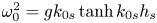 $\omega _0^2 = g k_{0s} \tanh k_{0s}h_s$ and
  $(2\omega _0)^2 = g k_{20s} \tanh k_{20s}h_s$, respectively.
The separation of the bound and free packets can be clearly seen as they propagate away from the step at  $x = 0$ m. The separation becomes obvious for gauge positions
  $x \geq 5$ m. The propagation speeds and directions of various packets are illustrated by the straight lines with arrows. Evidently,
  $c_{g,20s} < c_{g0s}$, so that the bound packet arrives first followed by the free superharmonic packet (cf. gauge 13 at
  $x=10$ m).
4.1.2. Free and bound subharmonics $\zeta ^{(20,1)}$

Compared with the superharmonic waves, the subharmonic waves have a smaller magnitude for case A5 shown in figure 4 (and likewise for the other three cases shown in appendix C). When the subharmonic bound packet, which takes the form of a set-down, experiences a depth transition, its magnitude increases, and a free ‘set-up’ is generated on the shallower side. Their combined effect has three aspects, as illustrated in figures 4 and 6. First, the free set-up propagates at (approximately) the shallow water speed  $\sqrt {gh_s}$, which is larger than the bound set-down that propagates at the group speed of the main carrier wave on the shallower side
  $c_{g0s}$ (
 $c_{g0s}< \sqrt {gh_s}$). This leads to the free set-up separating from the main packet and its set-down after a certain distance away from the step. Second, the magnitude of the effective set-down near the step on the shallower side becomes larger as we move away from the step and the free set-up propagates ahead faster. Third, the magnitude of the set-down becomes steady when the free and bound packets no longer overlap, as shown in figure 6.
For completeness, we note that agreement with theory in figure 4 ahead of the step is less good due to spurious subharmonic error waves associated with linear generation at the paddle (cf. Schäffer (Reference Schäffer1996) and the experiments of Calvert et al. (Reference Calvert, Whittaker, Raby, Taylor, Borthwick and van den Bremer2019)). The rapidly travelling free set-up is poorly absorbed by the beach at the end of the flume, is reflected and travels back, as shown by the rightmost arrow in figure 6.
4.2. Increased skewness near the depth transition
As noted in § 4.1, the maximum surface elevation can be significantly enhanced near the top of a depth transition due to second-order effects. As discussed in Li et al. (Reference Li, Zheng, Adcock, Lin and van den Bremer2021), there exists a peak location  $x_p$ that corresponds to the location where the second-order superharmonic bound and free waves are in phase and the crest elevation thus reaches a maximum. One direct consequence of this is that the surface elevations at this location are strongly vertically skewed. We illustrate this in figure 7, where the total surface elevation at the location where maximum crest elevation is observed is shown for three representative cases: A1, A2 and B2. Because the positions of the wave gauges are fixed, the maximum surface elevation measured in experiments may be different from the overall maximum. This is demonstrated in figure 7, where the surface elevations at the theoretically predicted peak locations are shown in figure 7(d–f). We do not have measurements at these theoretically predicted peak locations.

Figure 7. Vertically skewed waves for cases A1, A2 and B2 at the locations of maximum amplitude in the experiments (a–c) and in theory (d–f). The amplitude is scaled by the linear peak amplitude ( $A_s = |T_0|A_0$) measured at gauge 9. (a) A1:
  $h_d=0.55$ m,
  $f_0=0.6$ Hz,
  $x=1.1$ m. (b) A2:
  $h_d=0.55$ m,
  $f_0=0.65$ Hz,
  $x=1.1$ m. (c) B2:
  $h_d=0.75$ m,
  $f_0=0.7$ Hz,
  $x=1.1$ m. (d) A1: at
  $x_p=2.86$ m. (e) A2: at
  $x_p=2.16$ m. ( f) B2: at
  $x_p=1.06$ m.
Figure 7 illustrates that the crest elevation can be larger than the trough by  $75\,\%$,
  $60\,\%$ and
  $45\,\%$ for cases A1, A2 and B2, respectively. The additional elevation significant pushes the limits of the perturbation expansion, as evident from the locally non-monotonic behaviour in the trough in figure 7(d,e). Nevertheless, the good agreement between theory and experiments in figure 7(a–c) demonstrates that the theoretical model works well for the cases presented here (
 $\epsilon = 0.04\text {--}0.08$).
4.3. Quantitative comparison with theory and the role of depth
We now proceed to investigate the role of the most important non-dimensional parameters of the problem: the carrier wavelength relative to the deeper water depth  $k_0h_d$ and the depth ratio
  $h_s/h_d$. The scaled maximum crest elevation as a function of
  $k_0h_d$ is shown in figure 8 for the two depth ratios we have examined (
 $h_s/h_d=0.36$ and
  $0.53$), comparing experiments with theory. Several things can be noted from figure 8. First, there is generally good agreement between the theory and experiments for all
  $k_0h_d$ and for both depth ratios. The increase in maximum crest elevation is predominantly due to the superharmonic terms, with the subharmonic terms being small. Second, both superharmonic bound and free waves increase in magnitude as
  $k_0h_d$ decreases. The amplitude of the free waves is larger than that of the bound waves for
  $k_0h_d \lesssim 1.6$ for
  $h_s/h_d = 0.36$, but always smaller for
  $h_s/h_d = 0.53$. Third, the increase in maximum crest elevation is generally larger for a smaller depth ratio
  $h_s/h_d$ (figure 8(a) versus 8(b)). Fourth, owing to the fixed gauge positions, we are observing increases in maximum crest elevation of up to
  ${\sim }35\,\%$, but not the even larger increases of
  ${\sim }75\,\%$ predicted at the peak locations for the smallest depth ratio and small
  $k_0h_d$.

Figure 8. Maximum crest elevation at gauge 9 ( $x=0.90$ m) as a function of
  $k_0h_d$. The circles show (a) cases A1–A8 with
  $h_s/h_d=0.36$ (
 $h_s=0.20$ m,
  $h_d=0.55$ m) and (b) cases B2–B5 with
  $h_s/h_d=0.53$ (
 $h_s=0.40$ m,
  $h_d=0.75$ m).
4.4. Steep slopes compared to a step
In this section, we extend our study from a step to a slope. Specifically, we examine two steep slopes, a  $1\,{:}\,1$ slope and a
  $1\,{:}\,3$ slope (see table 2, cases C5 and D5, which we compare with case A5), and consider time series and maximum surface elevation in turn.
4.4.1. Time series
A time-series comparison is presented in figure 9, where the different harmonics are shown. The step and the two slopes demonstrate qualitatively the same physics with minor quantitative differences in amplitude and phase. This is confirmed in the zoomed-in time series in figure 9(d): all three experiments are in phase before the depth change (i.e. at gauge 1,  $x=-1.88$ m). Downstream of the depth change, at
  $x=1.10$ m shown in figure 9(e), there is a clear phase difference for the
  $1\,{:}\,3$ slope in the total, linear and superharmonic signals compared to the step and the
  $1\,{:}\,1$ slope, which remain in phase. We note that, at this location, the superharmonic phase difference is a result of the combined phase of the free and bound superharmonics. Further downstream of the depth change, at
  $x=14.0$ m shown in figure 9(f,g), there is an even greater phase difference observed for the free superharmonic packet (figure 9g) than for the bound superharmonic packet (figure 9g).

Figure 9. (a–c) Time series of the different harmonics at three gauge positions for three different slopes. (d–g) Zoomed-in versions of the same time series. In the figure,  $T_p = 1/f_0$ denotes the wave period of the carrier wave.
4.4.2. Maximum surface elevation amplitudes
Assessing the maximum crest elevation, figure 9 shows only small visual differences for the two slopes and the step. For a clearer assessment of the variation in amplitudes, post-processing was carried out to estimate the amplitude of the separated free and bound superharmonic packets for all of the cases with different slopes: cases A2–8 ( $1\,{:}\,0$), C2–8 (
 $1\,{:}\,1$) and D2–8 (
 $1\,{:}\,3$) in table 2. This was done using peak extraction applied to the Hilbert transform of the filtered superharmonic signal as described in appendix A.2. This approach enables a consistent estimate of the amplitudes of the packets to be obtained even when the free and bound harmonics are not fully separated. We note that the amplitude obtained from this technique should differ from the true like-for-like focused amplitude. However, this does not affect the validity of the comparisons.
The normalised separated amplitudes of the free, bound and total (sum of free and bound) superharmonic wavepackets are presented in figure 10 as a function of  $k_0h_d$. Also shown in figure 10 are the separated amplitude values obtained from three repeats of the
  $k_0h_d = 1.55$ cases for each of the slopes (A5, C5, D5). The right-hand panel of figure 10 shows a zoomed-in version of the separated harmonics corresponding to the black box in the main panel. Assessing the second-order bound superharmonics in figure 10, it is evident that the amplitudes are not greatly affected by the gradient of the slope. The free superharmonic wavepackets, however, appear to reduce in amplitude as the gradient reduces. This is observed consistently across
  $k_0h_d$ except for the highest value tested. The unchanged bound and smaller free harmonics result in a reduction in the total superharmonic amplitude with reduced slope gradient. Although relatively small differences are observed, steeper slopes are therefore expected to result in larger crest height values near the depth transition and are hence more likely to induce extreme wave events. Assessing the values of the repeats (right-hand panel) demonstrates that the extracted amplitude values are consistent.

Figure 10. Amplitudes of the free and bound superharmonic packets extracted from the experiments relative to the linear focused wave amplitude  $A_s =|T_0|A_0$ as a function of non-dimensional water depth
  $k_0h_d$ for different slopes. The right-hand panel shows a zoomed-in area for the cases for which repeated experiments have been carried out.
Despite the differences shown in figures 9 and 10, the overall trend is that the differences in both phase ( ${\lesssim }3\,\%$) and amplitude (
 ${\lesssim }5\,\%$) are small between the different depth transitions. This demonstrates that the theoretical model derived in Li et al. (Reference Li, Zheng, Adcock, Lin and van den Bremer2021) can be an effective model for second-order waves experiencing a steep slope.
5. Conclusions
In this paper we have examined experimentally the effect of an abrupt depth transition on the evolution of a surface gravity wavepacket that ‘feels’ the depth transition with a focus on the effects arising at second order in steepness. Experimental results for a step have been compared with the theoretical model derived in the companion paper (Li et al. Reference Li, Zheng, Adcock, Lin and van den Bremer2021), examining two depth ratios. Additionally, the effect of replacing a step by (steep)  $1\,{:}\,1$ and
  $1\,{:}\,3$ slopes has been examined. The following conclusions can be drawn.
First, we have experimentally validated the second-order narrow-banded wave theory derived in Li et al. (Reference Li, Zheng, Adcock, Lin and van den Bremer2021) for surface wavepackets experiencing an abrupt depth transition. The following new physics identified in Li et al. (Reference Li, Zheng, Adcock, Lin and van den Bremer2021) is observed experimentally here. As the main (linear) wavepacket propagates over the step, bound waves at second order change magnitude, and freely propagating wavepackets are released. Specifically, free superharmonics and subharmonics at second order are out of phase with their their bound counterparts and propagate at different speeds from the group velocity of the main (linear) packet. This leads to rich local behaviour near the top of a depth transition. The different harmonics overlap locally, and the superposition of those harmonics leads to an overall maximum crest amplitude at a location that we refer to as the ‘peak location’. The free components separate from the main packet after a certain distance.
Second, for a step, a quantitative comparison can be made between the maximum crest amplitude measured and predicted by theory. For the steepness considered here, the second-order theory, which agrees with the experimental results, suggests that the maximum wave amplitude can become as large as  $175\,\%$ of the incident linear focused wave amplitude at the peak location, mainly as a result of the superposition of different wave harmonics at up to second order in wave steepness. This leads to a surface elevation that is strikingly vertically skewed; the wave crest can be larger than the trough by
  $75\,\%$, a much greater difference than would be expected from bound waves alone. The authors conjecture that the vertically skewed surface elevation and the considerable amplification of the wave amplitude explain the local change in wave statistics for random waves observed near the top of the depth transition in a series of papers reviewed in Trulsen (Reference Trulsen2018). Future work will explore this further.
Finally, experiments with three different slopes (i.e. a step and  $1\,{:}\,1$ and
  $1\,{:}\,3$ slopes) have shown only minor changes in phase and amplitude of the second-order free superharmonic components. This suggests that the theoretical model derived in Li et al. (Reference Li, Zheng, Adcock, Lin and van den Bremer2021) can be an effective model for steep slopes, at least those with gradients larger than
  $1\,{:}\,3$.
Acknowledgements
S.D. acknowledges a Dame Kathleen Ollerenshaw Fellowship. T.S.v.d.B. acknowledges a Royal Academy of Engineering Research Fellowship. The authors would like to thank Mr A. Reynolds, Mr A. Oxenham, Dr K. Monk and Dr S. Stripling at the COAST laboratory for their help in planning and delivering the experiments.
Funding
This work has been supported by NSFC-EPSRC-NERC grants 51479114, EP/R007632/1 and EP/R007519/1 and a Flexible Fund grant from the UK & China Centre for Offshore Renewable Energy. Y.L. acknowledges the support from the Research Council of Norway via the FRIPRO mobility project 287389.
Declaration of interests
The authors report no conflict of interest.
Appendix A. Post-processing using frequency filtering and the separation of different wave harmonics
A.1. Filtering harmonics
To separate the linear, superharmonic and subharmonic components of the surface elevations, frequency-domain filters were applied. These were implemented by taking a single-sided fast Fourier transform of the surface elevation, then an inverse fast Fourier transform of the frequency components allocated to the harmonics. The lower and upper frequency bounds of these harmonics are taken, considering the bandwidth of the input spectrum, as
 \begin{equation} f_{{lower},N} = N f_0 - 2\delta,\quad f_{{upper},N} = N f_0 + 2\delta, \end{equation}
where  $N = 0$,
  $1$ and
  $2$ for subharmonic, linear and superharmonic wave components, respectively. This process is depicted in figure 11 for case A5 at gauge 9. The total time series corresponding to the total spectrum is shown, along with the separated harmonics. The corresponding frequency bounds used for the filtering process are indicated by the colours and the dashed lines in the energy density spectrum, which correspond to the colours of the presented filtered surface elevations.

Figure 11. Filtering approach for the extraction of wave harmonics demonstrated for case A5 at gauge 9.
A.2. Separation of free and bound superharmonics
As the superharmonic signal is made up of free and bound components, additional analysis is required to separate these, in order to compare their relative amplitudes (see figure 10). To achieve this, for each case a gauge is identified where the free and bound superharmonics are well separated. A Hilbert transform is then applied to the signal, and the locations and amplitudes of the peaks of the absolute Hilbert transform are identified. These peak values are taken as the representative amplitudes of the separated free and bound superharmonic wavepackets. This process is shown in figure 12 for case A3, where gauge 14 is used. The second peak is identified as the magnitude of the free superharmonic wavepacket due to its lower group velocity.

Figure 12. Filtering approach used to extract amplitudes of free and bound superharmonics shown for case A3 at gauge 14.
Appendix B. Error analysis and repeatability
This appendix quantifies the experimental errors. The potential errors in the wave gauge measurements are assessed in § B.1, with those from other sources (e.g. changes in water depth from evaporation, wavemaker non-repeatability, noise, etc.) assessed through repetition of experiments (§ B.2).
B.1. Wave gauge error
During experiments, calibration was carried out each morning using a three-point calibration. Gauges were positioned at known  $z$ positions of 0.05,
  $-0.05$ and 0 m and a linear fit applied between these positions and the measured voltages. The predicted surface elevations from this fit were compared with the known positions to provide a representative error, taken as the mean standard deviation (over all calibrations and every gauge) between the measured and predicted values. The resulting mean error value is
  $2.469\times 10^{-4}$ m with a standard deviation of
  $2.061\times 10^{-4}$ m (over all calibrations and every gauge). Gauge drift over a day was analysed in detail and found to be negligible.
B.2. Repeatability
To assess the repeatability of the tests, three repeats were carried out for four of the experiments defined in table 2: A2, A5, B1 and B2. The mean coefficient of determination between each repeat and every other repeat, averaged over all gauges, is shown in table 3. This is shown for the total measured time series, along with the filtered linear, super- and subharmonic components. Very high repeatability is observed, despite some repeats being carried out on different days. In general, slightly reduced repeatability is evident for the (much smaller) subharmonic components. The equivalent mean standard deviations are shown in table 4, noting that they roughly vary proportionally with the focused wave amplitude.
Table 3. Mean coefficients of determination between three repeats over and all gauges for cases A2, A5, B1 and B2 separated out by harmonics.

Table 4. Mean standard deviations between three repeats, and all gauges, for cases A2, A5, B1 and B2 separated out by harmonics.

Appendix C. Time histories for cases A2, B1 and B2
Three additional cases shown in figure 13 demonstrate qualitatively similar behaviour to case A5, including the local processes near the top of a depth transition and the release of free wavepackets as a result of waves interacting with the step.

Figure 13. Measured and theoretically predicted surface elevation separated out by harmonic at gauges 1, 9 and 14 for cases A2, B1 and B2. All surface elevations are scaled by the focused wave amplitude  $A_s =|T_0|A_0$ measured at gauge 9. The position (a,d,g) before the step, (b,e,h) near the step on the shallower side and (c, f,i) far downstream of the step.


 Open access