


Introduction
Cotton varieties with the glyphosate tolerance trait were first introduced to the Australian cotton industry in the 2000–2001 season and were rapidly adopted by the industry, with approximately 99% of cotton planted over the last decade including this trait (May, Monsanto Australia, personal communication). The widespread use of glyphosate in Australian cotton has led to high levels of weed control being achieved and has gone hand in hand with increasing yields, such that Australia continues to have the highest average cotton yields in the world (Dowling Reference Dowling2016).
However, an increasing number of weed species have developed resistance to glyphosate since 2000 (Heap Reference Heap2019), and weeds continue to be troublesome for cotton growers. The development of resistance to glyphosate has primarily occurred because of overreliance on glyphosate as the main method of weed control in fallows between cropping phases, and these resistant weeds have now become problematic during the cropping phase (Thornby et al. Reference Thornby, Werth and Walker2013). Weeds have been generally well managed in cotton, with most weeds present at densities well below one plant m−2 after weed control operations; volunteer cotton often is the only exception to this rule (Werth et al. Reference Werth, Boucher, Thornby, Walker and Charles2013).
Farmers have managed their weeds in cotton by adopting a low tolerance to weeds in crop and preventing seed set of weeds that survive a management operation, driving the seed bank down. This attitude of low tolerance to weeds, however, is becoming increasingly difficult to maintain on cotton farms as the occurrence of glyphosate-resistant weeds increases. Although a range of alternative herbicides remains available to cotton growers, none is as effective as glyphosate, and overreliance on the alternative chemistries will almost certainly result in weeds also developing resistance to these options. Managing weeds in irrigated cotton is made more difficult by asynchronous germination events, often making it challenging to determine the optimal timing for weed management inputs.
One approach to determining the optimal timing for managing asynchronous weed germinations in a glyphosate-resistant cotton crop to which glyphosate can be applied over the top from emergence to 22 nodes of crop growth is to define the critical period for weed control (CPWC) (Bukun Reference Bukun2004). The CPWC is the period of the season during which weeds need to be controlled to ensure yield losses due to weed competition do not exceed an identified yield-loss threshold (Fast et al. Reference Fast, Murdock, Farris, Willis and Murray2009; Korres and Norsworthy Reference Korres and Norsworthy2015; Webster et al. Reference Webster, Grey, Flanders and Culpepper2009). The yield-loss threshold is normally based on the cost of the weed control option to be used. The CPWC is determined for each weed and crop combination and relates to a specific level of weed competition (Bridges and Chandler Reference Bridges and Chandler1987; Papamichail et al. Reference Papamichail, Eleftherohorinos, Froud-Williams and Gravanis2002; Tursun et al. Reference Tursun, Datta, Budak, Kantarci and Knezevic2016). It is influenced by factors such as the time of weed and crop emergence (Webster et al. Reference Webster, Grey, Flanders and Culpepper2009), seasonal variation (Bukun Reference Bukun2004; Tingle et al. Reference Tingle, Steele and Chandler2003), plant nutrition (Buchanan and McLaughlin Reference Buchanan and McLaughlin1975; Tursun et al. Reference Tursun, Datta, Tuncel, Kantarci and Knezevic2015), and row spacing (Buchanan et al. Reference Buchanan, Crowley and McLaughlin1977; Rogers et al. Reference Rogers, Buchanan and Johnson1976; Tursun et al. Reference Tursun, Datta, Budak, Kantarci and Knezevic2016).
The CPWC is determined by identifying the critical time for weed removal (CTWR), the critical weed-free period (CWFP), and the yield-loss threshold. The CTWR is the period after crop emergence during which weeds can be allowed to compete with the crop without causing a yield loss exceeding the yield-loss threshold. The CWFP is the minimum period after crop emergence during which the crop must be maintained weed free to prevent a yield loss exceeding the threshold. The combination of the CTWR and the CWFP with the yield-loss threshold can be used to define the CPWC (Korres and Norsworthy Reference Korres and Norsworthy2015).
The CPWC has traditionally been determined for each weed and crop combination, but these experiments are both labor intensive and time consuming when multiple weeds are considered. Complications, such as hard-seeded weeds and asynchronous weed germination, can further confound the experiments. Alternatively, the CPWC can be determined for naturally occurring, mixed weed populations, although the results from these experiments are likely to be season and site specific (Buchanan et al. Reference Buchanan, Crowley and McLaughlin1977), with different combinations of weed species, germination timings, and weed pressure occurring in each experiment (Bukun Reference Bukun2004; Korres and Norsworthy Reference Korres and Norsworthy2015; Ma et al. Reference Ma, Yang, Wu, Jiang, Ma and Ma2016; Papamichail et al. Reference Papamichail, Eleftherohorinos, Froud-Williams and Gravanis2002; Tursun et al. Reference Tursun, Datta, Tuncel, Kantarci and Knezevic2015; Webster et al. Reference Webster, Grey, Flanders and Culpepper2009). Both approaches are challenging to apply to cotton production in Australia, where more than 70 weed species can be commonly found in the field and at least 40 species are considered to be problematic, ranging from prostrate weeds such as puncturevine (Tribulus terrestris L.), to potentially very large species, such as large thornapple (Datura ferox L.), sesbania [Sesbania cannabina (Retz.) Poir.], and common cocklebur (Xanthium strumarium L.) (Werth et al. Reference Werth, Boucher, Thornby, Walker and Charles2013). Other large weeds, such as Indian jointvetch (Aeschynomene indica L.) and velvetleaf (Abutilon theophrasti Medik.) are also present in some regions.
No CPWC has been established for large broadleaf weeds in high-yielding cotton in Australia. Recent work by Charles et al. (Reference Charles, Sindel, Cowie and Knox2019) demonstrated the potential for using mimic weeds to define weed competition, and this approach could be applied to determining the CPWC. Use of a mimic weed could give the advantages of better control over weed density, more uniform weed emergence, and better experimental repeatability. Ideally, mimic weeds should closely resemble their weedy analogues, allowing the results to be directly translated from mimic weed to real weed.
Large weeds can be competitive at relatively low densities. Ma et al. (Reference Ma, Yang, Wu, Jiang, Ma and Ma2016) found that velvetleaf densities as low as 0.25 plants m−1 of row reduced cotton growth and delayed crop development. Charles et al. (Reference Charles, Murison and Harden1998) reported even lower densities of common cocklebur and large thornapple causing economic damage in cotton in Australia. As weed density increases, generally the level of competition also increases, further reducing crop yields (Buchanan and Burns Reference Buchanan and Burns1971; Ma et al. Reference Ma, Yang, Wu, Jiang, Ma and Ma2016; MacRae et al. Reference MacRae, Webster, Sosnoskie, Culpepper and Kichler2013). However, intraspecific competition between weed plants also increases with increasing weed density and there is often a concurrent decrease in weed biomass per plant, although at a slower rate than the increase in weed density (Ma et al. Reference Ma, Yang, Wu, Jiang, Ma and Ma2016). This reduction in weed biomass per plant may not be reflected in other measures of weed size, such as weed height. Ma et al. (Reference Ma, Yang, Wu, Jiang, Ma and Ma2016) found that an increase in velvetleaf density led to shorter, thinner cotton plants, but taller velvetleaf plants, even though weed biomass per plant declined. MacRae et al. (Reference MacRae, Webster, Sosnoskie, Culpepper and Kichler2013) observed a linear relationship between weed density and weed biomass m−1 of row, with no evidence of a reduction in Palmer amaranth (Amaranthus palmeri S. Watson) plant size with increasing weed density from two to 10 weeds m−1 of row.
Weed density is an important aspect of weed competition that has not been fully accounted for in many competition studies (Smith et al. Reference Smith, Murray and Weeks1990). Buchanan et al. (Reference Buchanan, Crowley and McLaughlin1977) established both the CPWC and the minimum density of prickly sida (Sida spinosa L.) required to reduce the yield of cotton. Bridges and Chandler (Reference Bridges and Chandler1987) did the same for johnsongrass [Sorghum halepense (L.) Pers.]) and Tingle et al. (Reference Tingle, Steele and Chandler2003) for smellmelon (Cucumis melo var. dudaim Naud.). However, in none of these studies did the researchers consider the interaction of weed density and the CPWC.
In many other studies, the importance of weed density has largely been disregarded. Cardoso et al. (Reference Cardoso, Alves, Severino and Vale2011), for example, reported the relative abundance of weed species in a naturally occurring population, but did not report the actual weed density or biomass of the weeds, even though these measures were used to determine the relative abundance of the weeds. In many earlier studies, only the range of species present or the average weed density for the experiment was reported, often averaged over seasons (Buchanan and Burns Reference Buchanan and Burns1970; Buchanan and McLaughlin Reference Buchanan and McLaughlin1975; Rogers et al. Reference Rogers, Buchanan and Johnson1976; Snipes et al. Reference Snipes, Street and Walker1987). Other researchers have recorded weed biomass (Papamichail et al. Reference Papamichail, Eleftherohorinos, Froud-Williams and Gravanis2002; Webster et al. Reference Webster, Grey, Flanders and Culpepper2009), which is correlated with weed density (Ma et al. Reference Ma, Yang, Wu, Jiang, Ma and Ma2016; MacRae et al. Reference MacRae, Webster, Sosnoskie, Culpepper and Kichler2013), but have not reported weed density. Fast et al. (Reference Fast, Murdock, Farris, Willis and Murray2009), for example, reported Palmer amaranth biomass over time, but only gave the weed density averaged over four seasons.
This failure to fully account for weed density and biomass in many previous studies may be one of the factors leading to the site and seasonal variability in the results of many of these competition experiments (Korres and Norsworthy Reference Korres and Norsworthy2015; Ma et al. Reference Ma, Yang, Wu, Jiang, Ma and Ma2016). Other factors contributing to seasonal variability may include species differences and differences in weed emergence patterns (Robinson Reference Robinson1976a), environmental differences (Fast et al. Reference Fast, Murdock, Farris, Willis and Murray2009), rainfall (Rogers et al. Reference Rogers, Buchanan and Johnson1976; Tingle et al. Reference Tingle, Steele and Chandler2003), the presence of plant diseases (Buchanan et al. Reference Buchanan, Crowley and McLaughlin1977), soil nutrition, and other soil constraints (Buchanan and McLaughlin Reference Buchanan and McLaughlin1975; Tursun et al. Reference Tursun, Datta, Tuncel, Kantarci and Knezevic2015).
Although weed and crop interactions can be defined relatively easily in field experiments, all too often the results cannot be easily generalized to develop industry recommendations, because of the combination of diverse sites and season-specific factors. However, many of these constraints are less problematic in a fully irrigated crop, such as most cotton grown in Australia, where crop and weed germination is usually initiated by irrigation, and soil nutrition and moisture are largely nonlimiting throughout the season. The impact of seasonal temperature differences can also be diminished by using growing degree days (GDD) as the time measurement (Tursun et al. Reference Tursun, Datta, Budak, Kantarci and Knezevic2016; Webster et al. Reference Webster, Grey, Flanders and Culpepper2009). The objective of this study was to determine the CPWC for a large, mimic broadleaf weed in high-yielding irrigated cotton over a series of seasons and evaluate the impact of weed density on the CPWC.
Materials and Methods
Field studies were conducted over six seasons at the Australian Cotton Research Institute, Narrabri (30.12°S, 149.36°E; elevation 201 m), using commercial cotton cultivars Sicot 289 RRI in 2003–2004; Sicot 289 BR in 2004–2005; Sicot 80 BRF in 2005–2006, 2006–2007, and 2007–2008; and Sicot 71 BRF in 2015–2016. The soil was a heavy alluvial clay (fine, thermic, smectitic, Typic Haplustert). Cotton was planted at 15 seeds m−2 on September 30, 2003; October 4, 2004; October 19, 2005; October 6, 2006; October 8, 2007; and October 21, 2015. The cotton was grown on raised hills, 1 m apart in fully irrigated fields and fertilized with 180 kg N ha−1, in line with commercial practices. Irrigation was scheduled according to computer modelling of the crop’s requirements. Common sunflower, ‘Hyoleic 43,’ was planted in the 2003–2004, 2004–2005, and 2005–2006 seasons and ‘Hysun 38’ was planted in the later seasons at the specified densities and times in rows adjacent to and offset from the cotton rows by 100 mm. Plots were otherwise maintained weed free with trifluralin (Triflur X, 480 g ai L−1; Nufarm Australia, Melbourne, Victoria, Australia) at 1.1 kg ha−1, incorporated at preplanting. Glyphosate (Roundup Ready Herbicide, 690 g kg−1; Monsanto Australia, Melbourne, Victoria, Australia) at 1 kg ha−1 was applied POST as necessary over weed-free plots (2004–2005 season and later), and hand hoeing was performed as needed.
Experimental Design
The experiments used a split-plot design within a randomized, complete block design with four replications. Main plots were times of weed planting and subplots were times of weed removal and weed densities. Subplots were 4 rows wide (4 m) by 10 m long. Common sunflower seed was planted to achieve 0, 1, 2, 5, 10, 20, and 50 plants m−2, planted with the crop or at predetermined POST periods. Times of weed planting and weed removal were measured in GDD, using 15.5 C as the base temperature (Tursun et al. Reference Tursun, Datta, Budak, Kantarci and Knezevic2016). Times of weed planting and removal were targeted to occur at 150, 300, 450, 600, 750, and 900 GDD, but actual times were influenced by factors such as rainfall and irrigation scheduling. Not all weed densities and times of weed planting and removal occurred in all seasons, with weed emergence sometimes delayed by inadequate surface soil moisture at the time of planting, and not all target weed densities were achieved in all seasons.
The density of established weeds was counted on 1 m of row in each plot at the time of weed removal. Cotton was harvested at the end of each season using a modified commercial harvester with a single picking head, recording seed-cotton yield from the two central rows of each plot. Subsamples from one row were ginned using a single-saw gin to determine lint yield.
Statistical Analysis
Data were analyzed by ANOVA with replicate, year, time of weed interference and removal, and weed density as factors, using R, version 3.4.2, statistical software (Foundation for Statistical Computing, Vienna, Austria) with a significance level of P < 0.05. Analysis indicated no significant year effect or year interactions on relative lint yield (lint yield relative to the weed-free control in each season), allowing the data sets from the six seasons to be combined. Relative lint yield was significantly related to time of weed removal and interference, and weed density (P < 0.001). Data were then grouped into density categories such that the average density of each group equated as closely as possible to the nominal densities of 1, 2, 5, 10, 20, or 50 common sunflower plants m−2. Relative lint yield was regressed as a function of the time of weed removal or interference within each nominal weed density.
The effect of weed interference at each nominal weed density was modelled using the Gompertz function (Equation 1) (Korres and Norsworthy Reference Korres and Norsworthy2015):
 $$y = a\,ex{p^{ - ex{p^{b(T - c)}}}}$$
where y is the yield as a percentage of the weed-free control, a is the upper asymptote (constrained to 100%), b and c are constants, and T is the cumulative degree days since planting. T (Equation 2) was defined as:
 $$T = \sum {{{(t{min} + t{max} )} \over 2}} - {t_b}$$
where tmin and tmax are the daily minimum and maximum air temperatures, respectively, and t b is the base temperature of 15.5 C (Bukun Reference Bukun2004).
The effect of weed removals at each nominal weed density was modelled using the logistic function (Equation 3) (Korres and Norsworthy Reference Korres and Norsworthy2015):
 $$y = {a \over {1 + ex{p^{b\left( {T - c} \right)}}}}$$
where y is the yield as a percentage of the weed-free control, a is the upper asymptote, b and c are constants, and T is the cumulative degree days since planting.
These functions were extended to include actual weed density as a covariate. The extended Gompertz function (Equation 4) was:
 $$y = a\,ex{p^{ - ex{p^{b(T - c + dTW)}}}}$$
where d is an additional constant and W is the observed weed density.
The extended logistic function (Equation 5) was:
 $$y = {a \over {1 + ex{p^{b\left( {T - c + dTW} \right)}}}}$$
where d is an additional constant and W is the observed weed density.
Data for weed and crop height, and weed biomass were analyzed by ANOVA with replicate, year, time of weed removal, and weed density as factors, using a significance level of P < 0.05. Analysis indicated all year effects and year interactions were fully accounted for by the time of weed removal, allowing the data sets from the six seasons to be combined. Data were grouped into density categories and modelled using the Gompertz function (Equation 1) and an exponential model (Equation 6), and the Akaike information criterion used to determine the model of best fit for the data. The exponential model was:
 $$y = a + b\,ex{p^{cT}}$$
where y is crop height in cm, or weed or crop biomass in g plant−1 or g m−2; a, b, and c are constants, and T is the cumulative degree days since planting.
Results and Discussion
Cotton Lint Yield and Weed Density
Cotton yields varied over the six seasons, with average lint yields for the weed-free plots of 1,800, 2,110, 2,450, 1,540, 2,250, and 2,110 kg lint ha−1, in the 2003–2004, 2004–2005, 2005–2006, 2006–2007, 2007–008, and 2015–016 seasons, respectively. These yields were close to the average yield of Australian cotton for these years (Dowling Reference Dowling2016).
Common sunflower competed strongly with cotton. The CTWR curves fit to each weed density showed that when the weed germinated with the crop, high levels of competition commenced soon after crop emergence, with the curves rapidly declining toward 100% yield loss around mid-season (Figure 1). Season-long interference resulted in no harvestable cotton at densities of five or more common sunflower plants m−2. Even at the lowest density of 1 m−2, common sunflower still competed strongly with cotton, with season-long interference reducing cotton lint yield by 89%. Weeds that emerged early in the season after crop emergence were still highly competitive, as shown by the CWFP curves.
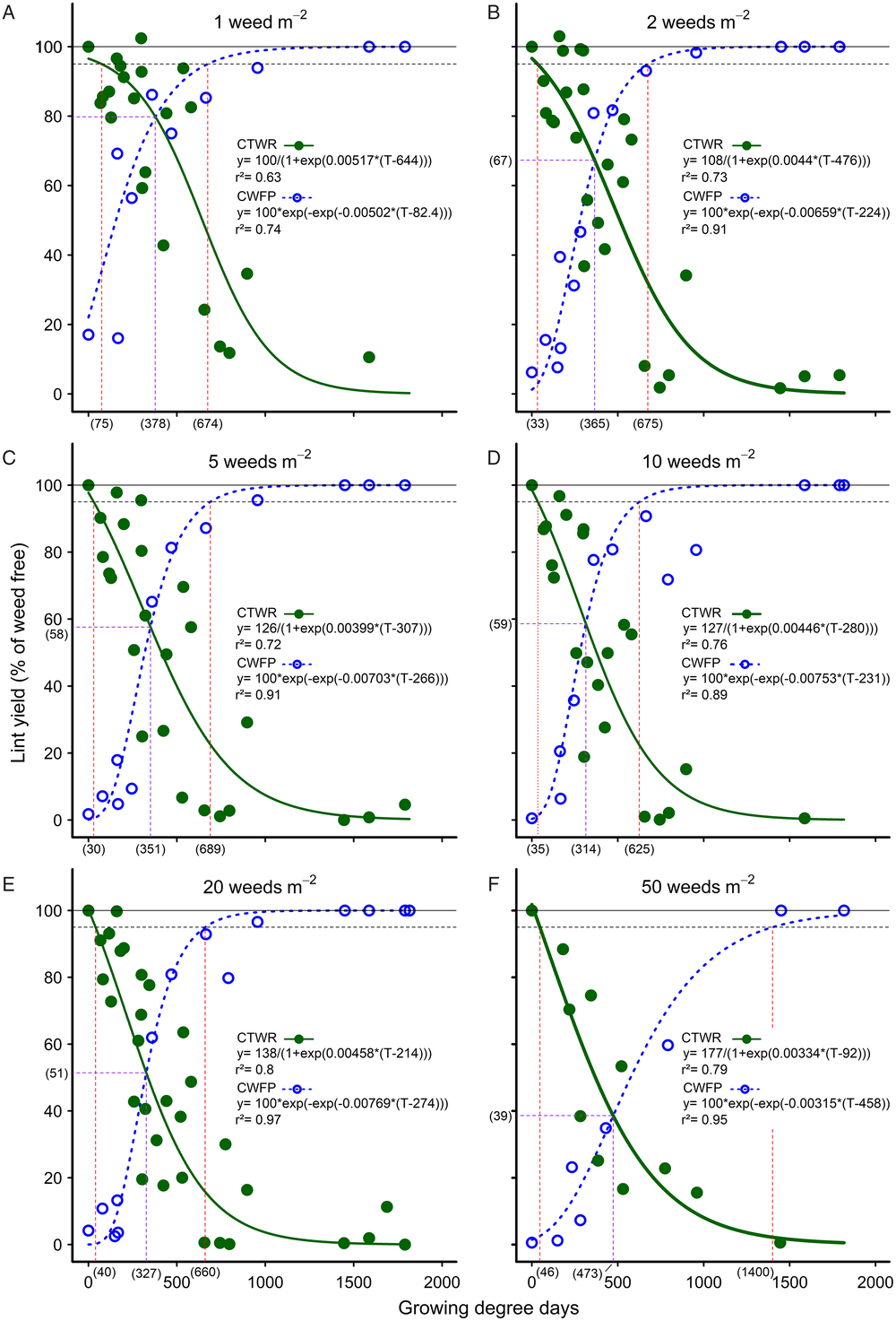
Figure 1. The influence of common sunflower interference durations—critical timing for weed removal (CTWR; green lines) and critical weed-free periods (CWFP; dashed blue lines)—on the cotton lint yield for densities of (A) 1, (B) 2, (C) 5, (D) 10, (E) 20, and (F) 50 weeds m–2. Parameters of the Gompertz (CTWR) and logistic (CWFP) functions are shown within the figures, where y is the lint yield and T the cumulative degree days since planting. Data points for the relationships are treatment means. The horizontal solid lines indicate the weed-free yield and the horizontal dashed lines give a nominal 5% yield-reduction threshold. The critical period for weed control (CPWC) is defined by the upper intersection of the CTWR and CWFP lines with the threshold. The limits of the derived CPWC curves are shown by the vertical dashed red lines and values bracketed below the x-axis. The point of minimal yield loss is shown by the dashed purple lines and bracketed values.
An arbitrary 5% lint-yield reduction threshold was applied (Ghosheh et al. Reference Ghosheh, Holshouser and Chandler1996), such that the CPWC was defined by the upper intersection of the CTWR and CWFP curves with the 5% threshold at each weed density. The critical periods so derived ranged from 75 to 674 GDD at one common sunflower plant m−2 to 40 to 660 GDD at 20 common sunflower plants m–2 and 46 to 1,400 GDD at 50 common sunflower plants m−2 (Figure 1A, 1E, and 1F, respectively). These results show little effect of weed density on the lower limit of the CPWC or on the upper limit of the CPWC at densities of one to 20 common sunflower plants m−2.
This lack of response to weed density, however, appears to be an artefact resulting from the form of the curves used. Webster et al. (Reference Webster, Grey, Flanders and Culpepper2009) proposed that another way of measuring the relative competitiveness of weed and crop was to consider the point of minimum yield loss from a single weed-control measure, that is, the point where the weed removal and weed interference curves intersect. This comparison shows that the point of minimum yield loss declined consistently with increasing weed density, from 20% yield loss with one common sunflower plant m−2 (Figure 1A) to 61% yield loss with 50 common sunflower plants m−2 (Figure 1F), corresponding to 378 GDD and 139 g weed biomass m−2, and 473 GDD and 547 g weed biomass m−2, respectively (Figure 2D). This result with one common sunflower plant m−2 was very similar to the results reported by Webster et al. (Reference Webster, Grey, Flanders and Culpepper2009) for Benghal dayflower (Commelina benghalensis L.) competing in cotton, where, for June-planted cotton in 2004, the point of minimum yield loss of 19% occurred at 174 g weed biomass m−2 and 373 GDD.
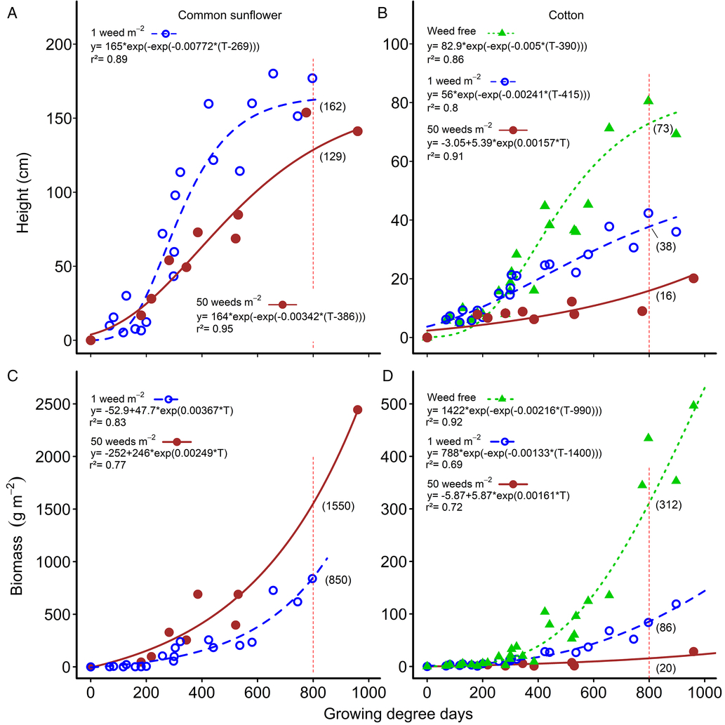
Figure 2. Changes in common sunflower and cotton height (A and B, respectively) and above-ground biomass (C and D, respectively) over the growing season for weed densities of 0 (weed free), 1, and 50 m−2. Parameters of the models are shown within the figure. Data points for the relationships are treatment means. Height and biomass values at mid season (800 growing degree days) are indicated by the vertical red dashed lines and bracketed values.
Nevertheless, although there was a consistent decline in the point of minimum yield loss with increasing weed density, there was no consistent effect of weed density on the CPWC for one to 20 weeds m−2. This lack of consistent response in our CPWC relationships reflects two components. First, the derived CPWC was very sensitive to the shape of the fitted curves as they approached the threshold. The upper end of the CTWR curve changed noticeably at the lowest density, resulting in an increase in the start of the CPWC at one common sunflower plant m−2 compared with other densities. Had a lower threshold been chosen, at say, 20% lint yield loss, the change in the critical period would have been much more clearly correlated to changing weed density, increasing from no critical period for one common sunflower plant m−2 to 148 to 934 GDD with 50 common sunflower plants m−2. This sensitivity to the shape of the curves as they approach the asymptote is fundamental to the type of curves used (i.e., logistic and Gompertz curves) and has not been an issue in most previous work, where the CPWC commenced several weeks after crop emergence and the maximum observed yield loss was much less than 100% (Cardoso et al. Reference Cardoso, Alves, Severino and Vale2011; Korres and Norsworthy Reference Korres and Norsworthy2015; Webster et al. Reference Webster, Grey, Flanders and Culpepper2009). We overcame this issue for the Gompertz curves by constraining the curves to asymptote at 100%. Such a constraint applied to the logistic curves, however, distorted the curves unacceptably. Consequently, the issue of sensitivity to curve shape is an inherent problem with logistic curves when highly competitive weeds are present, crop damage commences at or soon after crop emergence, and the maximum crop damage approaches 100% yield loss.
The second reason for the lack of response to weed density in the CPWC relationships is that the competitive effect of the weeds is not directly proportional to the density of weeds, because of increasing intraspecific competition between the weeds with increasing weed density. Thus, the level of competition experienced by the crop increased at a slower rate than the rate of increase of the weed density. This effect became increasingly important as weed density increased.
Plant Height and Biomass
There was little difference in weed height (Figure 2A) or weed biomass (Figure 2C) with increasing weed density up until approximately 300 GDD. Later in the season, weed height and biomass per plant decreased as weed density increased, but the changes were far less than the changes in weed density, as was observed with velvetleaf in cotton (Ma et al. Reference Ma, Yang, Wu, Jiang, Ma and Ma2016). At mid-season (800 GDD), weed biomass approximately doubled, from 850 g m−2 to 1,553 g m−2, as weed density increased 50-fold (Figure 2C). At the same time, weed height declined by only 21% (Figure 2C), but weed biomass per plant decreased by 96% from 841 g plant−1 at 1 plant m−2, to 34 g plant−1 at 50 weeds m−2, a 25-fold change in biomass. Similarly, crop height at mid season was reduced by 48% by a single common sunflower plant m−2, from 73 cm to 38 cm (Figure 2B). Increasing the weed density 50-fold to 50 common sunflower plants m−2 only reduced crop height by an additional 30% to 16 cm. Crop biomass at mid season was reduced by 73% by a single common sunflower plant m−2, from 312 to 86 g m−2 (Figure 2D). Increasing the weed density 50-fold to 50 common sunflower plants m−2 only reduced crop biomass by an additional 22% to 20 g m−2.
The decrease in common sunflower biomass per plant with increasing weed density followed the trend reported for johnsongrass (Bridges and Chandler Reference Bridges and Chandler1987) and velvetleaf up to nine weeds m−1 crop row (Ma et al. Reference Ma, Yang, Wu, Jiang, Ma and Ma2016) but was a much steeper curve than reported in these studies. At 300 GDD, the curve declined from 121 g plant−1 with one common sunflower plant m−2, reaching an asymptote of 14 g plant−1 and reaching 95% of this asymptote (20 g plant−1) at 20 weeds m−2 (Figure 3A). By 600 GDD, the initial part of the curve had become steeper again, reaching 95% of the asymptote of 55 g plant−1 at 11 weeds m−2 (Figure 3B). The curve became increasingly steep with time, by 900 GDD reaching 95% of the asymptote of 78 g plant−1 at five weeds m−2 (Figure 3C). These steeper curves relate to the much higher levels of competition in our experiments, with common sunflower densities of up to 50 weeds m−2 and mid-season weed biomass of up to 1,550 g m−2 (Figure 2D). With velvetleaf densities of up to 25 m−2 and end-of-season weed biomass of greater than 1,100 g m−2, Cortés et al. (Reference Cortés, Mendiola and Castejón2010) also observed much steeper relationships than reported by Bridges and Chandler (Reference Bridges and Chandler1987) and Ma et al. (Reference Ma, Yang, Wu, Jiang, Ma and Ma2016), although not as steep as in the current study, probably due to the lower levels of weed biomass in the earlier studies.
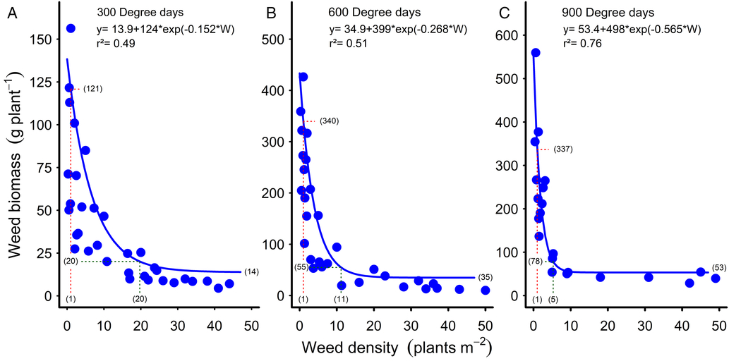
Figure 3. Reduction in common sunflower dry biomass with increasing weed density at (A) 300, (B) 600, and (C) 900 growing degree days. Parameters of the models are shown within the figures. Data points for the relationships are treatment means. Biomass values at one plant m−2 are indicated by the red dashed lines and bracketed values. Green dashed lines and bracketed values show the biomass and plant density at 95% of the asymptote. The weed biomass asymptote values are bracketed at the ends of the curves.
The steepness of the curves in our studies (Figure 3) indicates that very high levels of both intraspecific and interspecific competition were occurring at the higher weed densities (Firbank and Watkinson Reference Firbank and Watkinson1985; White and Harper Reference White and Harper1970). Self-thinning of the common sunflower population could be expected at these high weed densities (Deng et al. Reference Deng, Zuo, Wang, Fan, Ji, Wang, Ran, Zhao, Liu, Niklas, Hammond and Brown2012), as was observed by Robinson (Reference Robinson1976a) at much lower weed biomass levels than occurred in the current study. However, no reductions in either the common sunflower or cotton densities were observed over the course of the experiments beyond the mortality level of the plots with the lowest weed density, with plant survival probably enhanced by regular irrigation and high levels of soil nitrogen (Robinson Reference Robinson1976b).
Dynamic Relationships for Cotton Lint Yield
As an alternative approach to address the lack of consistent response of the CPWC to weed density at a 5% yield-loss threshold, we fit the data to extended Gompertz and logistic curves that included weed density as a covariate in the equations. These extended equations allowed a CPWC to be calculated for all densities in the experimental range of one to 50 common sunflower plants m−2. The equations also had the advantage of using actual weed densities, rather than the grouped densities of the earlier equations, making more efficient use of the data and creating a dynamic CPWC that can be more easily applied in the field. The CPWC estimated by these equations increased from 43 to 615 GDD for one common sunflower plant m−2 to 20 to 1,512 GDD for 50 common sunflower plants m−2, using a 5% yield-reduction threshold (Figure 4).
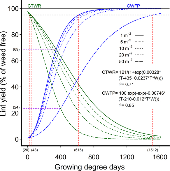
Figure 4. Dynamic relationships showing the influence of common sunflower interference durations—critical timing for weed removal (CTWR) and critical weed-free periods (CWFP)—on the relative cotton lint yield, using extended Gompertz (CTWR) and logistic (CWFP) functions including weed density as a covariate. Parameters of these models are shown within the figure. The derived relationships for common sunflower densities of 1, 5, 10, 20, and 50 m−2 are presented as examples. The horizontal solid line indicates the weed-free yield and the horizontal dashed line gives a nominal 5% yield-reduction threshold. The critical period for weed control (CPWC) is defined by the intersection of the CTWR and CWFP lines with the threshold. The CPWC for one and 50 common sunflowers m−2 are shown by dashed red lines. The limits of the CPWC are bracketed below the x-axis. The point of minimum yield loss from a single weed control input at one and 50 weeds m−2 is shown by the dashed purple lines and bracketed numbers.
The lower limit of the dynamic CPWC commenced between PRE and 11 d after crop emergence (DAE) for one common sunflower plant m−2, and between PRE and 6 DAE for 50 common sunflower plants m−2 over the six experimental seasons. The CPWC ended at 615 GDD (63 to 81 DAE) for one common sunflower plant m−2 and 1,512 GDD (136 DAE to full season) for 50 common sunflower plants m−2, with the CPWC ending after the application of the first crop defoliant in two of the six seasons.
The start of the our dynamic CPWC using a 5% yield-loss threshold was earlier than has been reported in many previous studies, commencing at or prior to crop emergence in four of six seasons. With a mixed population including the large weed common cocklebur, Bukun (Reference Bukun2004) reported the start of the CPWC at 100 to 150 GDD with a 5% yield-loss threshold, although that CPWC commenced before planting when Bukun (Reference Bukun2004) assigned a 2.5% threshold. Snipes et al. (Reference Snipes, Street and Walker1987) reported the start of the CPWC 14 to 28 d after planting with approximately eight common cocklebur plants m−2, similar to our 6 to 21 d after planting for eight common sunflower plants m−2, but many others recorded the start of the CPWC between 19 and 31 DAE (Cardoso et al. Reference Cardoso, Alves, Severino and Vale2011; Fast et al. Reference Fast, Murdock, Farris, Willis and Murray2009; Korres and Norsworthy Reference Korres and Norsworthy2015; Papamichail et al. Reference Papamichail, Eleftherohorinos, Froud-Williams and Gravanis2002).
The end of the CPWC was also later in our study than has been reported in many previous studies, extending late into the growing season for 50 common sunflower plants m−2 (1,512 GDD, or 136 DAE or more), with most other studies reporting the end of the CPWC at 42 to 84 DAE (Bukun Reference Bukun2004; Cardoso et al. Reference Cardoso, Alves, Severino and Vale2011; Korres and Norsworthy Reference Korres and Norsworthy2015; Papamichail et al. Reference Papamichail, Eleftherohorinos, Froud-Williams and Gravanis2002; Tursun et al. Reference Tursun, Datta, Tuncel, Kantarci and Knezevic2015). Tursun (2016), for example, calculated the end of the CPWC at 67 and 60 DAE, but the weeds were also less competitive in Tursun’s study, with a biomass of 1,340 and 1,310 g m−2 at 1,000 GDD (2012 and 2013, respectively), compared with 1,550 g m−2 mid season for 50 common sunflower plants m−2 in our study. Bukun (Reference Bukun2004) calculated the end of the CPWC at 77 to 84 DAE, but again, the weeds were less competitive, at 1,150 to 1,330 g m−2 at 1,000 GDD in this study. The CPWC extended to season long when a 2.5% threshold was used (Bukun Reference Bukun2004).
This combination of high weed densities, a highly competitive weed, and a high-yielding crop is a major contributing factor to the extended length of the dynamic CPWC observed in our studies. Cotton is an indeterminate plant, able to compensate for a high level of early-season damage (Wilson et al. Reference Wilson, Sadras, Heimoana and Gibb2003). However, the ability to compensate for damage is associated with delayed crop growth and crop maturity. It appears from our work that a high-yielding cotton crop is less able to compensate for damage later in the season than would be expected on the basis of earlier work, generally on much lower-yielding crops. Our crops, averaging 5,180 kg seed cotton ha−1, were more sensitive to mid- and late-season damage from weed competition than has previously been reported, resulting in an extended CPWC.
The very high densities of a larger weed used in these experiments, of up to 50 common sunflower plants m−2, also contributed to the prolonged dynamic CPWC observed, but increasing weed density did not have a strong influence on the CPWC, with high-yielding cotton sensitive to even a single large common sunflower plant m−2. A doubling in weed density from five to 10 weeds m−2 increased weed biomass at 800 GDD by only 10% (Figure 2C) and the length of the dynamic CPWC by 3 to 6 d (Figure 4). This limited response to increasing weed density is consistent with the finding of Ma et al. (Reference Ma, Yang, Wu, Jiang, Ma and Ma2016), who observed yield reductions from as few as 0.25 velvetleaf plants m−2, but recorded little change in cotton yield, with densities doubling from four to eight weeds m−2.
Implications for High-Yielding Crops
We conclude that high-yielding cotton crops are very sensitive to competition from a large broadleaf weed such as common sunflower, with the CPWC commencing at or near crop emergence. The duration of the CPWC extended to mid season or later, depending on weed density and the level of the yield-loss threshold chosen. We applied an arbitrary 5% yield-loss threshold to our data, but where the target weed is susceptible to glyphosate in a glyphosate-resistant cotton crop, a cost-based yield-loss threshold of less than 1% could be applied on the basis of 2019 commodity prices in Australia. A 1% yield-loss threshold extended the CPWC from before crop emergence through to 836 GDD (78–101 DAE) for one weed m−2, and from before crop emergence through to crop harvest for densities of 35 weeds m−2 and higher.
From the dynamic model, the minimum yield loss where a single weed control input was made during the season increased from 31% for one weed m−2 to 76% for 50 weeds m−2 (Figure 4), far exceeding a cost-based yield-loss threshold estimated at less than 1%. Consequently, where large broadleaf weeds are present, a high level of weed control must be maintained throughout much of the cropping season in high-yielding cotton to ensure crop losses do not exceed the cost of weed control. Although densities of fewer than one weed m−2 were not considered in our study, previous work has shown that season-long competition from densities as low as 0.005 large, broadleaf weeds m−2 can cause economic damage (Charles et al. Reference Charles, Murison and Harden1998) in Australian cotton, and weeds present at lower densities still need to be controlled to preserve fiber quality, to avoid difficulties at harvest, and to help manage herbicide resistance by driving down the weed seedbank over time (Korres and Norsworthy Reference Korres and Norsworthy2015).
Acknowledgments
We thank the many assistants who were involved in this project and Bruce McCorkell, biometrician, New South Wales Department of Primary Industries (DPI), for his help analyzing the data. We also gratefully thank Dr. Ian Taylor, Cotton Research and Development Corporation (CRDC), who initiated this work and the reviewers who contributed to the published paper. We gratefully acknowledge the support for this work by the New South Wales DPI, the University of New England, the CRDC, and the Australian Cotton Cooperative Research Centre. No conflicts of interest have been declared.


 Open access