


1. Introduction
Shallow water flows feature two dimensions in the horizontal plane that greatly exceed the vertical dimension (Jirka Reference Jirka2001). Such flows can be encountered in rivers, wetlands or along the shorelines of lakes and oceans. In open channels, the shallow flow is partly driven by the three-dimensional (3-D) turbulence induced by the channel bed and sidewalls. This 3-D turbulence involves various types of coherent structures scaled with viscous length, roughness height, distance  $z$ from the wall and with the flow depth $h$, including: (i) near-wall streaks in smooth-bed open-channel flows (OCFs) or wake eddies behind roughness elements in rough-bed OCFs; (ii) hairpin vortices (scaled with $z$); (iii) large-scale motions known as LSMs, with length of ${\approx}2h{-}4h$ (e.g. hairpin packets); and (iv) very-large-scale motions known as VLSMs or superstructures, with length up to 50 $h$ or even longer (e.g. Adrian & Marusic Reference Adrian and Marusic2012; Cameron, Nikora & Stewart Reference Cameron, Nikora and Stewart2017; Peruzzi et al. Reference Peruzzi, Poggi, Ridolfi and Manes2020; Zampiron, Cameron & Nikora Reference Zampiron, Cameron and Nikora2020).
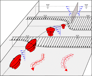
When subject to topographical singularities (embankment, two-stage channels, river confluence, side cavities, islands, etc.) or/and to lateral changes in hydraulic roughness, the shallow OCFs are transversely sheared. Examples include shallow wakes, jets and mixing layers. The focus of the present study is on the SMLs which manifest noticeable lateral transfer of mass, momentum, sediments, nutrients, contaminants and heat (Chu & Babarutsi Reference Chu and Babarutsi1988; Stocchino & Brocchini Reference Stocchino and Brocchini2010; Besio et al. Reference Besio, Stocchino, Angiolani and Brocchini2012; Mignot et al. Reference Mignot, Cai, Launay, Riviere and Escauriaza2016; Pouchoulin et al. Reference Pouchoulin, Le Coz, Mignot, Gond and Rivière2020; Proust & Nikora Reference Proust and Nikora2020; Cheng & Constantinescu Reference Cheng and Constantinescu2021). The mixing layers are characterized by a spanwise profile of time-averaged streamwise velocity  $U$ that typically exhibits an inflection point. Figure 1 outlines definitions of key variables (figure 1a) and comparative trends for SMLs and FMLs (figures 1b and 1c). An inflectional instability in the $U$-profile (Huerre & Rossi Reference Huerre and Rossi1998), termed Kelvin–Helmholtz instability, can generate large-scale vortical structures, conventionally termed Kelvin–Helmholtz coherent structures (KHCSs).
Hydrodynamic stability analyses of SMLs have been conducted for nearly forty years for flows either in rectangular open channels (Chu, Wu & Khayat Reference Chu, Wu and Khayat1983, Reference Chu, Wu and Khayat1991; Chen & Jirka Reference Chen and Jirka1998; Van Prooijen & Uijttewaal Reference Van Prooijen and Uijttewaal2002; Socolofsky & Jirka Reference Socolofsky and Jirka2004; Lam, Ghidaoui & Kolyshkin Reference Lam, Ghidaoui and Kolyshkin2019; Yu & Chu Reference Yu and Chu2020) or in compound (two-stage) channels (Alavian & Chu Reference Alavian and Chu1985; Chu et al. Reference Chu, Wu and Khayat1991; Ghidaoui & Kolyshkin Reference Ghidaoui and Kolyshkin1999). According to the stability theories, the onset and development of KHCSs in SMLs are dependent on the stability parameter  $S$ (Lam et al. Reference Lam, Ghidaoui and Kolyshkin2019), also termed the bed-friction number defined by Chu et al. (Reference Chu, Wu and Khayat1983) as
 \begin{equation} S = \frac{c_f}{2}\frac{\delta_v}{h} \frac{U_i}{U_s} = \frac{c_f \delta_v}{4h \lambda},\end{equation}
where  $c_f$ is the friction coefficient, $U_s=U_2-U_1$ is velocity shear between the two ambient streams (figure 1a), $U_i$ is velocity at the inflection point of the spanwise $U$-profile that is assumed to be equal to the average velocity $U_c = (U_1+U_2)/2$, $\delta _v = U_s/ ({\rm d} U/{{\rm d} y})_{max}$ is the vorticity thickness, ${({\rm d} U/{{\rm d} y})}_{max}$ is the velocity gradient at the inflection point and ${\lambda = (U_{2}-U_{1})/(U_{2}+U_{1})=U_s/(2U_c)}$ is the shear parameter (Brown & Roshko Reference Brown and Roshko1974).
The bed-friction number  $S$ appears in the Orr–Sommerfeld equation (Chu et al. Reference Chu, Wu and Khayat1983; Alavian & Chu Reference Alavian and Chu1985) or modified Orr–Sommerfeld equation for parallel flows (Chen & Jirka Reference Chen and Jirka1998; Ghidaoui & Kolyshkin Reference Ghidaoui and Kolyshkin1999), and accounts for the effect of bottom friction on the large-scale turbulent motion in shallow flow. Chu et al. (Reference Chu, Wu and Khayat1983) showed that a SML with parallel streams and a constant across the channel streamwise pressure gradient, is stable from large-scale spanwise disturbance for $S\geq S_c = 0.12$. In addition, the experiments of Chu & Babarutsi (Reference Chu and Babarutsi1988) showed that the growth rate of the SML width, ${\rm d} \delta _v / {{\rm d}\kern0.06em x}$, which reduces with distance from the splitter plate (figure 1b), was dependent on the local $S$-value as follows:
 \begin{equation} \frac{{\rm d} \delta_v}{{\rm d}\kern0.06em x} = 2\alpha \lambda,\end{equation}
where the entrainment coefficient  $\alpha = \alpha _0 (1-S/S_c)$ for $S < S_c$ and $\alpha = 0$ for $S \geq S_c$, and with $\alpha _0$ = 0.18 and $S_c$ = 0.09. Importantly, they also showed that for $S \geq S_c = 0.09$, the spanwise fluctuating motion vanished (Chu & Babarutsi Reference Chu and Babarutsi1988, figure 9).

Figure 1. Key parameters of the shallow mixing layers (SMLs), with free mixing layers (FMLs) serving as reference flows: (a) spanwise profile of the time-averaged streamwise velocity  $U$, where $U_1$ and $U_2$ are characteristic velocities of the two ambient streams, $U_i$ is velocity at the inflection point that equals average velocity $U_c =(U_1+U_2)/2$ for FMLs, $y_i$ is the spanwise position of $U_i$, $\delta _v =(U_2-U_1)/({\rm d} U/{{\rm d} y})_{max}$ is the vorticity thickness; (b) streamwise evolution of $\delta _v$; and (c) streamwise evolutions of $y_i$, spanwise position $y_c$ of $U_c$ and spanwise position $y_t$ of the extreme in turbulent shear stress $\overline {-u'v'}$.
A second important control parameter of the SMLs is the bed-friction length scale  $h/c_f$, as experimentally observed by Chu & Babarutsi (Reference Chu and Babarutsi1988). Unlike conventional FMLs, for which velocities $U_2$ and $U_1$ are constant along $x$-axis (Pope Reference Pope2000), SMLs feature a streamwise decrease in $U_2$ combined with an increase in $U_1$, which results in a decrease in $U_s U_c = U_2^2-U_1^2$ under the effects of shallowness and bed friction. Based on their simplified analytical consideration, Chu & Babarutsi (Reference Chu and Babarutsi1988) proposed an exponential relationship for $U_{2}^2-U_{1}^2$
 \begin{equation} \frac{{U_2}^2-{U_1}^2}{{U_{2,0}}^2-{U_{1,0}}^2} = \frac{U_s U_c}{U_{s,0} U_{c,0}} = \exp({-}x^{*}), \end{equation}
where  $U_1=U_{1,0}$ and $U_2=U_{2,0}$ at $x = x_0$, and $x^*= x c_f /h$ is the streamwise coordinate normalized by the bed-friction length scale $h/c_f$. This length scale is also invoked by Chu & Babarutsi (Reference Chu and Babarutsi1988) when considering the normalized vorticity thickness ${\delta _v^* = c_f \delta _v/(2h \lambda (x_0))}$ as a function of $x^*=x c_f/h$, where $\lambda (x_0)$ is calculated at $x = x_0$. These authors found that their data on $\delta _v^*$ collapsed around a single curve. Later on, a similar collapse was observed in the experiments of Uijttewaal & Booij (Reference Uijttewaal and Booij2000). Based on these experiments, Van Prooijen & Uijttewaal (Reference Van Prooijen and Uijttewaal2002) proposed the following formula for modelling the SML width:
 \begin{equation} \delta_v (x) = \alpha \frac{U_{s0}}{U_c} \frac{h}{c_f}\left(1-\exp \left(-\frac{c_f}{h}x \right)\right)+ \delta_{v_0},\end{equation}
which was obtained by (i) assuming that  $U_c$ in (1.3) was constant that resulted in ${U_s=U_{s0} \exp (-x^*)}$, and (ii) integrating (1.2) along $x$-axis using a constant entrainment coefficient $\alpha = 0.085$. In addition, drawing on the definition of thickness $\delta _v^*$ by Chu & Babarutsi (Reference Chu and Babarutsi1988), but using local value of $\lambda$ instead of the initial value $\lambda (x_0)$, Cheng & Constantinescu (Reference Cheng and Constantinescu2020) employed in their numerical simulations the normalized vorticity thickness as
 \begin{equation} \delta_v^* = \frac{1}{\lambda} \frac{c_f \delta_v}{2h} = 2 S,\end{equation}
and they found that, for parallel flows,
 \begin{equation} \delta_v^*= 0.09 x^*\quad \text{for} \ x^* < 1.5 \quad \text{and} \quad \delta_v^*= 0.0364 {x^*}^3 \quad \text{for} \ x^* > 2.\end{equation}
 A third important control parameter of the SMLs is the shear parameter  $\lambda$. First, in the benchmark experiments of Chu & Babarutsi (Reference Chu and Babarutsi1988), it was found that the initial growth rate of the SML width follows a relationship
 \begin{equation} \left(\frac{{\rm d} \delta_v}{{\rm d}\kern0.06em x}\right)_{x_0} = 0.36 \frac{U_{2,0}-U_{1,0}}{U_{2,0}+U_{1,0}} = 0.36 \lambda (x_0),\end{equation}
which is consistent with (1.2) considering that  $S = 0$ and $\alpha = \alpha _0 = 0.18$ at $x = x_0$. Note that this growth rate is twice as large as the nominal rate for the FMLs (Brown & Roshko Reference Brown and Roshko1974, (5.3))
 \begin{equation} \left(\frac{{\rm d} \delta_v}{{\rm d}\kern0.06em x}\right)_{x_0} = 0.181 \lambda (x_0). \end{equation}
Second, the shear parameter  $\lambda$ is a parameter that characterizes the stability of SMLs in the same way as bed-friction number $S$ (Socolofsky & Jirka Reference Socolofsky and Jirka2004; Yu & Chu Reference Yu and Chu2020), see e.g. the stability diagrams of SMLs in the plane ( $S$,
$S$,  $\lambda$) of Socolofsky & Jirka (Reference Socolofsky and Jirka2004, figure 8). Third, Cushman-Roisin & Constantinescu (Reference Cushman-Roisin and Constantinescu2020) found that $\lambda (x_0)$ was involved in the streamwise development of the spanwise location $y_m$ of the border between the fast and slow streams that preserves initial discharges $Q_1$ and $Q_2$, with $y_m$ assumed to be the SML centre. They found that the evolution of $y_m$ was governed by
 \begin{equation} \frac{W_1^2}{y_m^2}-\left(\frac{U_{2,0}}{U_{1,0}}\right)^2 \frac{(W_2)^2}{(W-y_m)^2}=\left(1-\left(\frac{U_{2,0}}{U_{1,0}}\right)^2\right) \exp({-}x^*),\end{equation}
where  $W_1$ and $W_2$ are the widths of the two streams at $x = x_0 = 0$, $W$ =
$W$ =  $W_1$ + $W_2$ is the channel width and $U_{2,0}/U_{1,0}$ is the velocity ratio of the incoming streams with ${U_{2,0}/U_{1,0} = (1+\lambda (x_0))/(1-\lambda (x_0))}$. Note that (1.9) was derived from a mass conservation equation together with the exponential decay of $U_sU_c$ (1.3). Fourth, the shear parameter $\lambda$ was found to control the emergence and development of KHCSs in SMLs for streamwise-depth-uniform and non-uniform flows in three different compound open-channel facilities (Proust et al. Reference Proust, Fernandes, Leal, Rivière and Peltier2017; Proust & Nikora Reference Proust and Nikora2020). Near the flume entrance, KHCSs can emerge if
 \begin{equation} \lambda \geq \lambda_c,\end{equation}
with  $\lambda _c \approx 0.3$, above which KHCS length scales increase with $\lambda$ (Proust & Nikora Reference Proust and Nikora2020), irrespective of the shallowness level, i.e. flow depth. This effect was also confirmed by 3-D eddy-resolving simulations by Chatelain & Proust (Reference Chatelain and Proust2020) of the flows studied by Proust & Nikora (Reference Proust and Nikora2020). The presence of an inflection point in the $U$-profile is a necessary condition for Kelvin–Helmholtz instabilities to occur (Rayleigh's theorem, e.g. Huerre & Rossi Reference Huerre and Rossi1998), while $\lambda \gtrapprox 0.3$ was found to be the second condition required for the emergence of KHCSs in compound channel flows (Proust et al. Reference Proust, Fernandes, Leal, Rivière and Peltier2017). Last, for FMLs, Brown & Roshko (Reference Brown and Roshko1974) found that the growth rate of KHCSs, denoted as ${\rm d} \delta _{vis.}/{{\rm d}\kern0.06em x}$ (where $\delta _{vis.}$ is the ‘visual’ thickness of the FML based on shadowgraphs of KHCSs) was proportional to $\lambda$ for a fixed value of density ratio $\rho _1/\rho _2$ between the ambient streams. For $\rho _1/\rho _2$ = 1 (three test cases),
 \begin{equation} \frac{{\rm d} \delta_{vis.}}{{\rm d}\kern0.06em x} = 0.38 \lambda,\end{equation}
which gives  $\delta _{vis.} / (x-x_0) = 0.38 \lambda$ assuming that $U_s$ and $U_c$ are constant between $x$ and $x_0$. The growth rate ${\rm d} \delta _{vis.}/{{\rm d}\kern0.06em x}$ is thus higher than the growth rate of the vorticity thickness (1.8). It is interesting to notice that all measured visual grow rates ${\rm d} \delta _{vis.}/{{\rm d}\kern0.06em x}$ correspond to $\lambda > \lambda _c = 0.3$ (Brown & Roshko Reference Brown and Roshko1974, figure 7) for $\rho _1/\rho _2$ in the range 1/7–7.
The present laboratory study is underpinned by the previous research on SMLs ranging from the pioneering works of Chu et al. (Reference Chu, Wu and Khayat1983), Alavian & Chu (Reference Alavian and Chu1985) and Chu & Babarutsi (Reference Chu and Babarutsi1988) to the most recent works of Cheng & Constantinescu (Reference Cheng and Constantinescu2020, Reference Cheng and Constantinescu2021), some elements of which are presented above. We have studied SMLs developing in a wide open channel with a hydraulically smooth bed. The novelty elements of this laboratory work include: (i) varying the initial shear parameter  $\lambda$ from 0 to a maximum value in the range 0.6–1 for four different levels of shallowness (flow depths $h$) and bed friction (length scale $h/c_f$); (ii) investigating the effect on the SML features of an increasingly strong spanwise time-averaged flow (arising from the increase in initial $\lambda$); and (iii) investigating the streamwise evolution of SMLs from their early development behind the splitter plate until their relaxation towards flow uniformity across the channel (i.e. $U_1=U_2$) and along the streamwise direction (using a tilted flume).
The first objective of the present study is to determine which parameters control the SML features based on the time-averaged velocity field (i.e. spanwise profile of the velocity  $U$, width $\delta _v$, growth rate of $\delta _v$, spanwise position of the SML centre and decay of $U_s U_c$). Particular attention is paid to the effect of an increasing time-averaged spanwise flow on the SML features (in addition to the effects of bed-friction length scale $h/c_f$ and shear parameter $\lambda$ previously described), as the spanwise base flow motion is assumed to be absent in the known stability theories of SMLs from Chu et al. (Reference Chu, Wu and Khayat1983) to Yu & Chu (Reference Yu and Chu2020). The second objective is to determine what drives (i) the emergence and development of the large-scale turbulent coherent structures (KHCSs, LSMs and VLSMs), and (ii) the bulk turbulence statistics. As for KHCSs, we intend to clarify the effects of flow depth $h$ (e.g. Uijttewaal & Booij Reference Uijttewaal and Booij2000; Cheng & Constantinescu Reference Cheng and Constantinescu2020, Reference Cheng and Constantinescu2021), bed-friction number $S$ (e.g. Chu et al. Reference Chu, Wu and Khayat1983; Alavian & Chu Reference Alavian and Chu1985; Chu & Babarutsi Reference Chu and Babarutsi1988; Socolofsky & Jirka Reference Socolofsky and Jirka2004; Lam et al. Reference Lam, Ghidaoui and Kolyshkin2019; Yu & Chu Reference Yu and Chu2020) and shear parameter $\lambda$ (e.g. Socolofsky & Jirka Reference Socolofsky and Jirka2004; Proust et al. Reference Proust, Fernandes, Leal, Rivière and Peltier2017; Proust & Nikora Reference Proust and Nikora2020; Yu & Chu Reference Yu and Chu2020) on the emergence, development, and length scales of the KHCSs. In addition, we want to relate the fate of the KHCSs to the normalized spanwise turbulent flux $\overline {u'v'}/\overline {u'^2}$, which is the simplest index of the turbulence structure, according to Townsend (Reference Townsend1976). Regarding LSMs and VLSMs, we want to explore their developments in the presence of a SML and without it, focusing on the effects of shear parameter $\lambda$ (Proust & Nikora Reference Proust and Nikora2020), spanwise time-averaged flow and streamwise secondary currents of time-averaged flow (Proust & Nikora Reference Proust and Nikora2020; Zampiron et al. Reference Zampiron, Cameron and Nikora2020).
Section 2 describes the tilted open-channel flume used in the experiments and presents the experimental set-up, flow conditions and measuring techniques. A general characterization of the streamwise flow development is given in § 3, including: spanwise distributions of the streamwise velocity  $U$, spanwise velocity $V$, momentum fluxes $UV$ and Reynolds stresses $\overline {u'v'}$; Froude numbers and flow depths in the two streams; examination of the time-averaged flow structure behind the splitter plate covering wake–mixing layer co-existence in weakly sheared flows (WSFs, to be defined in § 2.2); and secondary currents generated due to the presence of the splitter plate. The streamwise evolutions of the SML features based on the time-averaged flow are analysed in § 4 including: shear parameter $\lambda$, difference in the squared velocities $U_2^2-U_1^2$, vorticity thickness $\delta _v$, relative vorticity thickness $\delta _v/h$ and spanwise location of the SML centre for a range of its definitions. The large-scale coherent structures (KHCSs, LSMs and VLSMs) and bulk turbulence statistics are studied in § 5. In particular, we have explored: (i) the emergence of the KHCSs and their length scales behind the splitter plate; (ii) the effect of the bed-induced turbulence on the shear layer turbulence all along the measurement domain; (iii) the vertical non-uniformity of the turbulence statistics and KHCS length scales; and (iv) the development of LSMs and VLSMs in both uniform and sheared flows. Finally, the main outcomes of this study are summarized in § 6.

Figure 2. Open-channel flume: (a) view downstream (experiments with a working length  $= 18\ {\rm m}$ and a working width $= 2\ {\rm m}$ (right-hand 2/3 of the total flume width) with bed and sidewalls made of glass); (b) sketch of a cross-section (view downstream), in which $h_1$ and $h_2$ are the flow depths at $y = 0.5\ {\rm m}$ and 1.5 m, respectively; (c) sketch of the inlet flow conditions viewed from upstream, in which $Q_1$ and $Q_2$ are the inflow discharges in the right-hand and left-hand tanks; (d) flow near the splitter plate for $Q_1= 5$ l s $^{-1}$ and $Q_2 = 55$ l s $^{-1}$, view upstream; (e) flow near the splitter plate for $Q_1 = 3$ l s $^{-1}$ and $Q_2 = 27$ l s $^{-1}$, top view.
2. Experiments
2.1. Experimental facility
The experiments were conducted in an 18 m long and 2 m wide open-channel flume (figure 2) at the Hydraulics and Hydro-morphology Laboratory (HHLab) at INRAE, Lyon-Villeurbanne, France. The bottom and sidewalls of the rectangular channel are made of glass (figure 2a). The flume bed slope in the longitudinal direction  $S_0$ is $1.04\times 10^{-3}$. The flume is equipped with two independent inlet tanks (1.7 m long and 1 m wide each). Each tank is supplied with water through a tower with a constant water level reservoir. The flow rate in the left-hand tank ( $Q_2$) and the flow rate in the right-hand tank ( $Q_1$) are monitored with two independent flow meters. The flow partition is maintained until the trailing edge of a 50 cm long and 2.2 mm thick vertical splitter plate (figure 2c–e). A Cartesian right-handed coordinate system is used in which the $x$-axis is in the longitudinal direction parallel to the flume bottom, the $y$-axis is in the lateral direction and the $z$-axis is perpendicular to the flume bed (figure 2b,c). The system origin is defined as: $x= 0$ at the splitter plate trailing edge; $y = 0$ at the right-hand sidewall; $z = 0$ at the channel bottom. The downstream end of the flume is at $x = 17.25\ {\rm m}$ where a vertical weir enables the water surface elevation to be controlled.
2.2. Flow conditions
The inflow conditions of the 20 test cases are presented in table 1 (third to fifth columns). Each test case is identified by its values of right-hand inflow discharge  $Q_1$ and left-hand inflow discharge $Q_2$ (figure 2c). Four values of the total flow rate $Q = Q_1+Q_2$ were used (120, 60, 30 and 14 l s $^{-1}$) to vary flow depth $h$ and bed-friction length scale $h/c_f$. With a channel length to flow depth ratio $L/h = 196\unicode{x2013}720$, some of the test cases studied cover both the transition and quasi-equilibrium regimes of the SML defined by Cheng & Constantinescu (Reference Cheng and Constantinescu2020, Reference Cheng and Constantinescu2021). For each $Q$-value, the experiments started with uniform flow conditions. They were obtained by injecting equal discharges $Q_1$ and $Q_2$ in the two inlet tanks, and by setting the height of the downstream weir to obtain a constant time-averaged flow depth in the streamwise direction. Once the depth-uniform flow case ( $Q_1=Q_2$) was studied for a given $Q$-value, sheared flow cases were created by varying the flow partition between the two inlet tanks (with $Q_1 < Q_2$) keeping the height of the downstream weir unchanged. The initial shear parameter ${\lambda }$ at the flume entrance ( $x = 0.06$ m) ranged from 0 (uniform flow) to 0.6–1 (depending on the flow rate $Q$). The $\lambda$-values at $x = 1.65$ m are given in table 1, while the variation ranges of $\lambda$ from $x = 0.65$ m to $15.65\ {\rm m}$ are reported in table 2.
Table 1. Inflow conditions of the test cases: total flow rate  $Q$ and right-hand and left-hand inflow discharges $Q_1$ and $Q_2$. Flow parameters measured at $x = 1.65\ {\rm m}$: flow depths $h_{1}$ and $h_{2}$ at $y = 0.5\ {\rm m}$ and 1.5 m respectively, time-averaged streamwise velocities $U_{2}$ and $U_{1}$ measured at $z/h=0.5$, average velocity ${U_{c}=(U_{2}+U_{1})/2}$, velocity shear ${U_{s}=U_{2}-U_{1}}$, shear parameter ${\lambda =(U_2-U_1)/(U_2+U_1)}$, bed-friction coefficients in the slow and fast streams $c_{f1}$ (with $1/\sqrt {c_{f1}} = -4 \log (1.25/(4Re_1 \sqrt {c_{f1}}))$) and $c_{f2}$ (with $1/\sqrt {c_{f2}} = -4 \log (1.25/(4Re_2 \sqrt {c_{f2}}))$) , Froude numbers $Fr_1 = |U_{1}|/\sqrt {gh_{1}}$ and ${Fr_2 = |U_{2}|/\sqrt {gh_{2}}}$, Reynolds numbers ${Re_1 = |U_{1}|h_{1}/\nu }$ and ${Re_2 = |U_{2}|h_{2}/\nu }$. Here, WSF, MSF and HSF refer to weakly, moderately and highly sheared flow, respectively (see § 2.2).

Table 2. Variation ranges of the flow depths  $h_1$ and $h_2$, velocity shear ${U_{s}=U_2-U_1}$, average velocity $U_c = (U_2+U_1)/2$, shear parameter $\lambda =(U_2-U_1)/(U_2+U_1)$, vorticity thickness to flow depth ratio ${\delta _v/h}$ (with $\delta _v=(U_2-U_1)/({\rm d} U/{{\rm d} y})_{{max}}$ and $h = (h_1+h_2)/2$), bed-friction coefficients $c_f = (c_{f1}+c_{f2})/2$, $c_{f1}$ (with $1/\sqrt {c_{f1}} = -4 \log (1.25/(4Re_1 \sqrt {c_{f1}}))$) and $c_{f2}$ (with $1/\sqrt {c_{f2}} = -4 \log (1.25/(4Re_2 \sqrt {c_{f2}}))$), ratio ${h/c_f}$, bed-friction number $S = c_f \delta _v/ (4h \lambda$), maximum value of the spanwise velocity $|V^*|=|V|/U_c$ across the channel and maximum value of root mean square of the streamwise velocity fluctuation $\sqrt {\overline {{u^{'}}^{2}}}^*=\sqrt {\overline {{u^{'}}^{2}}}/U_c$. Here, N.D.: not defined.

In our considerations in the follow-up sections, we will distinguish three types of sheared flows, depending on the magnitude of initial  $\lambda$ and the streamwise change in $\lambda$ . The WSFs are defined as flows with initial $\lambda < \lambda _c \approx 0.3$, which are likely to be free of KHCSs (Proust et al. Reference Proust, Fernandes, Leal, Rivière and Peltier2017; Proust & Nikora Reference Proust and Nikora2020). The highly sheared flows (HSFs) are defined as flows with $\lambda$ consistently exceeding 0.3 between $x = 0.06\ {\rm m}$ and $x = 3.65\ {\rm m}$. The moderately sheared flows (MSFs) represent an intermediate case of flows with initial $\lambda > 0.3$ that is quickly falling below 0.3 between $x = 0.06\ {\rm m}$ and $x = 3.65\ {\rm m}$. The shear levels (i.e. WSF, MSF or HSF) are reported in table 1.
2.3. Measurements
2.3.1. Water depth
Water surface elevations were measured using an ultrasonic sensor manufactured by Baumer (UNDK 20IG903/S35A), with a standard measurement error of approximately 0.2 mm. Measurements were taken at a spatial interval of 0.1 m in the streamwise direction between  $x = 0.50\ {\rm m}$ and 16.50 m (161 measuring locations), at two spanwise positions $y = 0.5\ {\rm m}$ and 1.5 m (two longitudinal transects for each flow case). At each measuring point, the acquisition duration was 180 s at a sampling frequency of 50 Hz. The ultrasonic sensor was also used to perform a topographical survey of the channel bed. Flow depth was obtained as the difference between air heights measured by the sensor without and with water for a given position ( $x$,
$x$, $y$).
$y$).
2.3.2. One-point velocity measurements
One-point velocity measurements were conducted using a 3-D Nortek Vectrino $+$ acoustic Doppler velocimeter (ADV), with a side looking probe. The sampling volume was 5 cm away from the probe, and could be approximated as a cylinder 6 mm in diameter and 7 mm in height. At each measuring point, the three instantaneous velocities ( $u$,
$u$,  $v$,
$v$,  $w$) were recorded for 300 s at a rate of 100 Hz. The flow was seeded with 40 $\mathrm {\mu }$m polyamide particles to increase both the signal-to-noise ratio and the correlation level within the measuring volume. The velocity data were despiked using the procedure of Goring & Nikora (Reference Goring and Nikora2002). Relying on the experiments of Proust & Nikora (Reference Proust and Nikora2020) on SMLs in a compound channel that were carried out in the same flume employing similar procedures, the sampling standard errors for the mean flow parameters and turbulence statistics were approximately: 1 $\%$, 9 $\%$ and 16 $\%$ for the time-averaged velocities, $U$,
$U$,  $V$ and $W$, respectively; 3 $\%$, 2 $\%$ and 3 $\%$ for the turbulence intensities $\sqrt {\overline {{u'}^2}}$, $\sqrt {\overline {{v'}^2}}$ and $\sqrt {\overline {{w'}^2}}$; and 10 $\%$ for the Reynolds shear stress $-\overline {u'v'}$.
Spanwise profiles of velocity were measured at 9 to 11  $x$-positions and at mid-flow depth (elevation $z/h \approx 0.5$). In the spanwise direction, point measurements were taken at an interval of 10 mm inside the mixing layer, and 50 mm outside, for the early stage of development of the mixing layers (61 $y$-positions across the channel). Further downstream, an interval of 50 mm was used for the whole spanwise profile (37 $y$-positions).
In addition, for case 35-85 (table 1), velocity measurements were carried out in a cross-section (7  $z$-elevations and 61 $y$-positions for each $z$-value) at $x = 3.65$ m and 11.65 m. Last, a number of vertical profiles of velocities were measured at an interval of 6 mm along $z$-axis (13 $z$-elevations) for 60-60 and 35-85, to explore the shallowness and bed-friction effects on flow structure, and to detect the presence of likely streamwise helical secondary currents in the vicinity of the splitter plate.
2.3.3. Two-point velocity measurements
Two-point velocity measurements were carried out using two ADVs with side looking probes. First, they were aimed at characterizing the longitudinal and spanwise length scales of the KHCSs, also using an acquisition duration of 300 s at a rate of 100 Hz. The ADV probes were firstly aligned with the  $y$-axis at a given $x$-position at the same elevation $z/h = 0.5$. A fixed probe was measuring at the inflection point of the $U$-profile while the second probe was moving, point by point, along the $y$-axis, across the low-speed stream. Then, the ADV probes were aligned with the $x$-axis at the spanwise position of the inflection point (for a given $x$-position) at $z/h = 0.5$. The upstream probe was fixed while the second probe was moving point-by-point downstream. Lastly, the ADV probes were placed along the $z$-axis, the fixed probed was measuring at the inflection point at mid-depth, and the second probe was moving along the $z$-axis (this probe was shifted 10 cm away from the fixed probe in the spanwise direction). Second, the two-point velocity measurements were used to identify the long-range velocity fluctuations, namely the LSMs and VLSMs. For that purpose, the acquisition duration was increased to six hours at a rate of 100 Hz. At a given $x$-position (0.65 m, 3.65 m or 11.65 m), the ADV probes were simultaneously measuring at $y = 0.5\ {\rm m}$ and 1.5 m at $z/h = 0.5$. This was done for cases: 07-07, 05-09 (WSF) and 03-11 (HSF); 15-15, 13-17 (WSF) and 07-23 (HSF); 30-30, 25-35 (WSF) and 15-45 (HSF); 60-60, 50-70 (WSF) and 35-85 (HSF).
2.3.4. Identification of the characteristic length scales of the KHCSs
Characteristic length scales of the KHCSs are determined based on spatial correlations of spanwise velocity fluctuations  $v^{\prime }$ using the two-point velocity measurements. The streamwise correlation function is defined as
 \begin{equation} R_{yy}^x(x,\epsilon_x ) = \frac{\overline{v^{\prime} (x) v^{\prime}(x+\epsilon_x)}}{\sqrt{\overline{v^{\prime 2} (x)} \overline{v^{\prime 2}(x+\epsilon_x)}}},\end{equation}
where  $x$ is the position of the upstream fixed probe, $\epsilon _x$ is spatial lag in the $x$-direction between fixed and moving probes.
The spanwise spatial correlation function is similarly defined as
 \begin{equation} R_{yy}^y(y,\epsilon_y) = \frac{\overline{v^{\prime} (y) v^{\prime}(\kern0.7pt y+\epsilon_y)}}{\sqrt{\overline{v^{\prime 2} (y)} \overline{v^{\prime 2}(\kern0.7pt y+\epsilon_y)}}}.\end{equation}
 Figure 3(a) shows examples of spatial correlation function of the fluctuation of spanwise velocity  $v^{\prime }$ in the streamwise direction for a HSF populated by strong KHCSs (case 5-55) and a WSF (25-25) in which KHCSs are absent. Figure 3(b) shows examples of the correlation function across the SML on the slow stream side for a MSF (20-40) and a HSF (15-45), both populated by KHCSs, highlighting an increase in the correlation level with increasing shear parameter $\lambda$. The characteristic scales of the KHCSs are defined as spatial lags corresponding to a particular correlation level (e.g. McDonough Reference McDonough2007). The characteristic streamwise scale, denoted as $\delta _x^{CS}$, corresponds to the spatial lag $\epsilon _x$ between probes when $R_{yy}^x$ crosses zero for the second time, e.g. $\delta _x^{CS} = 0.8\ {\rm m}$ for 05-55 in figure 3(a). The scale $\delta _x^{CS}$ corresponds, approximately, to the 3/4 of the spacing between two KHCSs in the streamwise direction (see figure 4(b) for 05-55 at $x = 3.65\ {\rm m}$). The characteristic spanwise scale of KHCSs, denoted as $\delta _y^{CS}$, corresponds to the spanwise distance from the inflection point to the $y$-value within the slow stream where $R_{yy}^y$ reaches 0.10 (arbitrary correlation level, low but higher than the noise level), e.g. $\delta _y^{CS} = 0.37\ {\rm m}$ for 20-40 in figure 3(b).

Figure 3. Examples of spatial correlation functions of the spanwise velocity fluctuations  $v'$. The fixed probe is located at $x = 3.65\ {\rm m}$ and $z/h = 0.5$ and the second probe is moving point by point at the same elevation (a) along the streamwise direction (2.1) or (b) along the spanwise direction (2.2), the horizontal continuous line indicating $R_{yy}^y$ = 0.10.

Figure 4. Shear parameter  ${\lambda = (U_{2}-U_{1})/(U_{2}+U_{1})}$ as a function of the streamwise position $x$ (a); the dashed line indicates ${\lambda _c = 0.3}$. Detection of KHCSs using dye tracer injected at the inflection point in the $U$-profile, at $x = 3.65\ {\rm m}$ (b) and $x = 5.65\ {\rm m}$ (c) for representative test cases $Q_1$- $Q_2$ (e.g. 03-11 refers to inlet discharges ${Q_1 = 3 \, \rm {l\, s}^{-1}}$ and ${Q_2 = 11\ \text {l s}^{-1}}$).
Last, the vertical spatial correlation function that we used in our study is defined as
 \begin{equation} R_{yy}^z(z,\epsilon_z) = \frac{\overline{v^{\prime} (z) v^{\prime}(z+\epsilon_z)}}{\sqrt{\overline{v^{\prime 2} (z)} \overline{v^{\prime 2}(z+\epsilon_z)}}}.\end{equation}
2.3.5. Detection of KHCSs using a dye tracer
The position of the inflection point in the  $U$-profile (which is supposed to be the location of the core of the KHCSs) was identified by fitting the data with polynomial functions (of degree 3 behind the splitter plate, and of degree 5 further downstream). Dye tracer (potassium permanganate) was then injected at the inflection point to detect the possible presence of KHCSs. Figures 4(b) and 4(c) show photographs taken from above with an injection point at $x = 3.65\ {\rm m}$ and $x = 5.65\ {\rm m}$, respectively, along with the local values of the shear parameter $\lambda$ and flow depth $h$ at each $x$-position. When KHCSs are detected, each photograph is taken at a time when the KHCSs have a maximum lateral extension. Figure 4(a) additionally shows the changes in the shear parameter $\lambda$ along the flume.
3. Streamwise flow development: a general view
3.1. Spanwise distributions of the time-averaged streamwise velocity
Figure 5 shows spanwise distributions of the time-averaged streamwise velocity  $U$ scaled by the average velocity $U_c$. Velocity $U_{1}$ is defined as (i) the streamwise velocity averaged across the plateau region of $U =f(y)$ outside the SML on the low-speed side (see e.g. all cases with $Q = 30$ l s $^{-1}$ at $x = 0.65\ {\rm m}$ in figure 5(a)) or (ii) the minimum velocity across the slow stream in the absence of a plateau of $U$ (see e.g. case 00-14 at $x = 3.65\ {\rm m}$ in figure 5(b)). In a similar way, velocity $U_{2}$ is defined as (i) the streamwise velocity averaged across the plateau region of $U$ outside the SML on the high-speed side or (ii) the peak streamwise velocity across the fast stream in the absence of a plateau of $U$. Note that, to normalize velocity $U$, the velocity scale $U_c$ is more suitable than the velocity shear $U_s$ used for FMLs (Pope Reference Pope2000), as $U_s$ tends towards zero for SMLs far away from the flume entrance (figure 5c). Last, it should be noticed that case 00-14 features a recirculating flow zone near the flume entrance on the slow stream side. This is reflected by the negative values of $U^*$ (figure 5a) and positive values of $V^*$ (see § 3.2, figure 6) at $x = 0.65\ {\rm m}$. The fast stream in this case behaves like a ‘jet’ that laterally transfers momentum to the dead water zone and triggers the formation of a rotational cell with a vertical axis.

Figure 4 (cntd). Shear parameter  ${\lambda = (U_{2}-U_{1})/(U_{2}+U_{1})}$ as a function of the streamwise position $x$ (a); the dashed line indicates ${\lambda _c = 0.3}$. Detection of KHCSs using dye tracer injected at the inflection point in the $U$-profile, at $x = 3.65\ {\rm m}$ (b) and $x = 5.65\ {\rm m}$ (c) for representative test cases $Q_1$- $Q_2$ (e.g. 05-55 refers to inlet discharges $Q_1 = 5\ \rm {l\, s}^{-1}$ and $Q_2 = 55\ \text {l s}^{-1}$).
3.2. Spanwise distributions of the time-averaged spanwise velocity
Although the two incoming streams are parallel, a noticeable spanwise flow can be observed passed the splitter plate, as shown in figure 2(e) for case 03-27 (for which dye tracer was poured at the splitter plate trailing edge). Figure 6 shows spanwise distributions of the time-averaged spanwise velocity  $V$ scaled by $U_c$. The maximum values across the flow of $|V^*|=|V|/U_c$, denoted as Max $|V^*|$, are reported in table 2. For the MSFs and HSFs (with initial $\lambda >0.3$), Max $|V^*|>0.1$ and thus the streams behind the splitter plate cannot be considered as parallel. For the most sheared flows, the peak $V$-values can reach 33 %–55 % of $U_c$ (table 2). The assumption $V \ll U$ usually made in stability analysis is therefore not applicable for the MSFs and HSFs. For the latter, the discrepancy between inflow velocity and equilibrium velocity in a tilted open channel ( $U = 1/n h_n^{2/3} S_0^{1/2}$, where $h_n$ is the normal flow depth for a given $Q$-value), can be significant. This results in a noticeable mass redistribution across the flow in the upstream part of these shear flows. Note that such a spanwise flow is not observed within unbounded FMLs, where the spanwise exchanges of fluid are essentially due to the horizontal vortices and vortex merging. Last, we investigated the link between the magnitude of the spanwise mean flow and the possible driving parameters of the SMLs (see § 1). The spanwise mean flow was found to be mostly driven by shear parameter $\lambda$ in the upstream part of the SMLs. As shown in figure 7(a), at $x = 0.65\ {\rm m}$, Max( $V^*$) increases with $\lambda$ without any influence of the total flow rate, i.e. of flow depth $h$ and bed-friction length scale $h/c_f$. Similar results were obtained at $x = 3.65\ {\rm m}$ (not shown here). Note that the effect of a spanwise hydrostatic pressure gradient (quantified by flow depth difference $h_2\unicode{x2013}h_1$) on the spanwise flow is another factor influencing the magnitude of the spanwise flow (figure 7b).

Figure 5. Spanwise profile of the time-averaged streamwise velocity  $U^*=U/U_c$ at $z/h=0.5$ at $x = 0.65\ {\rm m}$ (a), $x = 3.65\ {\rm m}$ (b) and $x = 11.65\ {\rm m}$ (c). All cases with total discharge $Q = 14$, 30, 60 and 120 l s $^{-1}$. The standard error in $U$ is approximately 1 $\%$.
$\%$.

Figure 6. Spanwise profiles of the time-averaged spanwise velocity  $V^*=V/U_c$ at $z/h=0.5$ at: $x = 0.65\ {\rm m}$ (a), $x = 3.65\ {\rm m}$ (b) and $x = 11.65\ {\rm m}$ (c). The standard error in $V$ is approximately 9 $\%$.
$\%$.

Figure 7. Peak value of the time-averaged spanwise velocity  $|V^*=V/U_c|$ across the SMLs at $x = 0.65\ {\rm m}$ as a function of shear parameter $\lambda$ (a) and normalized flow depth difference $|h_2-h_1|/[(h_2+h_1)/2]$ (b) for $Q = 14$ l s $^{-1}$ ( $*$), 30 l s $^{-1}$ ( $\bullet$), 60 l s $^{-1}$ ( $\Box$) and 120 l s $^{-1}$ ( $\triangle$).
3.3. Spanwise exchange of the streamwise momentum
The strong time-averaged spanwise flow observed for MSFs and HSFs is accompanied by an equally strong transfer of momentum as illustrated by the values of  $|{U}^*{V}^*|$ in figure 8 for $Q = 120$ l s $^{-1}$ and $30$ l s $^{-1}$, which are compared with the Reynolds stresses $-\overline {u'v'}^* = -\overline {u'v'}/U_c^2$. Importantly, these momentum fluxes by the time-averaged flow are predominant with respect to the fluxes by turbulent diffusion, as also observed by Sukhodolov, Schnauder & Uijttewaal (Reference Sukhodolov, Schnauder and Uijttewaal2010) within SMLs behind a splitter plate in a river with a sandy bed (where the slow stream was generated by a spanwise porous obstacle). This would suggest that the turbulent structures could play a minor role on the growth rate of SML width $\delta _v$ along the whole measurement domain.

Figure 8. Spanwise exchange of streamwise momentum by the time-averaged flow  $|{U}^*{V}^*|$ and Reynolds shear stress $-\overline {u'v'}^*=-\overline {u'v'}/U_c^{2}$ at $z/h=0.5$, at $x = 0.65\ {\rm m}$ (a), $x = 3.65\ {\rm m}$ (b) and $x = 11.65\ {\rm m}$ (c), for cases with total discharge $Q = 120$ l s $^{-1}$ and 30 l s $^{-1}$. The standard error in $\overline {u'v'}$ is approximately 10 $\%$.
$\%$.
3.4. Froude numbers in the two streams
Based on streamwise velocities  $U_1$ and $U_2$ and flow depths $h_1$ and $h_2$ (measured at $y = 0.5\ {\rm m}$ and 1.5 m, figure 2(b)), the Froude numbers in the two streams ${Fr_1 = |U_{1}|/\sqrt {gh_{1}}}$ and ${Fr_2 = |U_{2}|/\sqrt {gh_{2}}}$ can be calculated at the $x$-positions where $U_1$ and $U_2$ were measured. The changes in ${Fr_2}$ and ${Fr_1}$ from $x=0.06\ {\rm m}$ to 15.65 m are presented in figure 9, and their values at $x = 1.65\ {\rm m}$ are reported in table 1. The slow stream is always subcritical, i.e. $Fr_1 < 1$. Some HSFs exhibit a spanwise juxtaposition of a subcritical slow stream and a supercritical fast stream for small $x$-positions. Along the $x$-axis, the transition from supercritical to subcritical flow is accompanied by an undular jump (§ 3.5).

Figure 9. Streamwise profiles of the Froude numbers in the slow stream  ${Fr_{1}=|U_1|/\sqrt {gh_1}}$ and in the fast stream ${Fr_{2}=|U_2|/\sqrt {gh_2}}$ from $x = 0.65\ {\rm m}$ to $x = 15.65\ {\rm m}$.
3.5. Flow depths in the two streams
The flow depths  $h_1$ and $h_2$ measured at ${x = 1.65\ {\rm m}}$ are reported in table 1, and their minimum and maximum values between $x = 0.65\ {\rm m}$ and 15.65 m are given in table 2. The streamwise changes in $h_1$ and $h_2$ are shown in figure 10. For a given $Q$-value, flow depth $h$ is normalized by the spatial average along the $x$- and $y$-axes of the water depth of the depth-uniform flow case (denoted as $\langle h^u \rangle _{x,y}$), as follows:
 \begin{equation} h^* = \frac{h}{\langle h^u \rangle_{x,y}}.\end{equation}
Figure 10. Streamwise changes in the normalized flow depth  $h^*$ (3.1) from $x = 0.5\ {\rm m}$ to $x = 16.5\ {\rm m}$ at spanwise positions $y = 0.5\ {\rm m}$ ( $\times$) and $y =1.5\ {\rm m}$ ( $\circ$). The standard error in flow depth $h$ is approximately 0.2 mm.
The uniform flow cases ( $Q_1=Q_2$) feature low-amplitude variations in $h^*$ around 1, which are mostly due to the variations in the bed topography around the average bottom level (of the order of $\pm$0.5 mm). For the non-uniform cases, the streamwise changes in $h^*$ are far more dependent on the initial value of the shear parameter $\lambda$ than on the total discharge $Q$. For instance, the four highest sheared flows (20-100, 05-55, 03-27, 00-14) feature the same variation range in $h^*$ either on the low-speed side (0.8–1) or the high-speed side (0.6–1). In the fast stream, the strong oscillations in $h^*$ are due to an undular jump that reflects the streamwise transition from supercritical flow to subcritical flow (figure 9), as also observed by Montes & Chanson (Reference Montes and Chanson1998) for a comparable range of Froude numbers ( $Fr_2$-values in the range 1.0–1.7 in figure 9). This transition occurs owing to the streamwise decrease in velocity $U_2$ under the effects of bed friction (as will be seen in § 4.2) and of the spanwise expansion of the fast stream into slow stream region (figures 5 and 6). It should be also noted that the control of the streamwise changes in $h^*$ by the initial shear parameter $\lambda$ irrespective of the $Q$-value is consistent with the data in figure 7(a).
3.6. Wake–mixing layer co-existence for WSFs
Near the flume entrance (figure 5a), a local velocity deficit can be observed in the  $U^*-$distribution between $y = 0.95\ {\rm m}$ and $1.05\ {\rm m}$ for the uniform cases ( $Q_1=Q_2$) and some WSF cases (05-09, 13-17 and 25-35). This velocity deficit manifests the presence of the splitter plate wake for low or zero values of $\lambda$, as also observed by Mehta (Reference Mehta1991) for FMLs, by Constantinescu et al. (Reference Constantinescu, Miyawaki, Rhoads, Sukhodolov and Kirkil2011) for two flows merging at a river confluence and by Proust et al. (Reference Proust, Fernandes, Leal, Rivière and Peltier2017) for SMLs in compound open channels. The absence of a wake for MSFs and HSFs can be explained by the significant spanwise time-averaged flow behind the splitter plate (figure 6a). This spanwise flow plays an important role in the redistribution of mass between streams, and also of momentum owing to the high values of $-U^*V^*$ that are an order of magnitude higher than the values of the Reynolds stress $-{\overline {u'v'}}^*$ (figure 8). Figure 5(a) additionally shows that the local velocity deficit is increasingly noticeable as the flow depth decreases (from $Q = 120$ to 14 l s $^{-1}$, see e.g. the uniform cases). This could be due to the decreasing influence of the helical secondary currents (with a longitudinal axis) going out from the inlet tanks and formed due to turbulence anisotropy and heterogeneity in the vicinity of the corners between vertical splitter plate and the channel bed (secondary currents will be analysed for cases 60-60 and 35-85 in detail in § 3.7). These secondary currents could contribute to the lateral redistribution of mass and streamwise momentum for the uniform flows and WSFs.
3.7. Helical secondary currents vs depth-averaged spanwise flow
Figure 11(a) shows vertical distributions of the spanwise mean velocity  $V$ for uniform case 60-60. Six centimetres and 65 cm downstream of the splitter plate, the $V$-distributions reflect the presence of a helical secondary current cell with a longitudinal axis spanning over the depth, going out from the rectangular inlet tank and further strengthened in flow regions adjacent to the bed–splitter plate corners. These secondary currents are Prandtl's secondary flows of the second kind originating from the turbulence anisotropy induced by the tank bottom and inlet separation wall (extended by the splitter plate). Further downstream at $x = 3.65\ {\rm m}$ and $x = 11.65\ {\rm m}$, secondary currents appear to vanish, with both $V$-values and depth-averaged spanwise velocity $V_d$ being close to zero. For the HSF 35-85 (figure 11b), the secondary current cell still exists just behind the splitter plate (data at $x = 0.06\ {\rm m}$). However, the secondary currents are quickly replaced by a noticeable depth-averaged spanwise flow at $x = 3.65\ {\rm m}$ with $V_d = -3$ cm s $^{-1}$, reflecting a net mass flux toward the slow stream. At $x = 11.65\ {\rm m}$, the $V$-distribution indicates the presence of transverse motions, which likely reflect the flow recovery from the presence of strong spanwise flow due to the high initial value of $\lambda$.
4. The SML features based on the time-averaged flow
4.1. Shear parameter  $\lambda$

The longitudinal changes in the shear parameter  $\lambda$ are shown in figures 4(a) and 12. The $\lambda$-parameter accounts for the velocity shear between streams and the average velocity across the SML that is also considered as the convection velocity for large-scale structures in FMLs (Brown & Roshko Reference Brown and Roshko1974). It is interesting to compare the streamwise evolution of $\lambda$ for flows with the same initial $\lambda$-value but various bed-friction length scales $h/c_f$, a predominant control parameter of the velocities $U_1$ and $U_2$ (see Chu & Babarutsi (Reference Chu and Babarutsi1988) and § 4.2). This can be done for cases 03-11, 07-23, 15-45 and 30-90, for which $\lambda = 0.46\unicode{x2013}0.48$ at $x = 0.65\ {\rm m}$ (table 2 and figure 12) and $h/c_f$ ranges from 5 to 25 m. At $x = 11.65\ {\rm m}$, the $\lambda$-values are 0.01, 0.09, 0.18 and 0.28 for these cases, respectively, demonstrating that the relaxation rate towards flow uniformity decreases with increasing $h/c_f$.

Figure 11. Vertical distributions of the time-averaged spanwise velocity  $V$ for uniform flow 60-60 (a) and HSF 35-85 (b). The standard error in $V$ is approximately 9 $\%$.
$\%$.

Figure 12. Streamwise changes in the shear parameter  ${\lambda =(U_{2}-U_{1})/(U_{2}+U_{1})}$ from $x = 0.06\ {\rm m}$ to $15.65\ {\rm m}$ at elevation ${z/h=0.5}$. The dashed line indicates ${\lambda _c = 0.3}$.
4.2. Difference in the squared velocities $U_2^2-U_1^2$

The relationship (1.3) was obtained from the momentum conservation equations (4.1) and (4.2) in the two ambient streams outside the SML, where the spanwise exchange of streamwise momentum is assumed to be negligible
 \begin{gather} U_2\frac{{\rm d}{U_2}}{{\rm d}\kern0.06em x} + \frac{1}{2}\frac{c_{f2}}{h} {U_2}^2 + \rho g \frac{{\rm d}h_2}{{\rm d}\kern0.06em x}-\rho g S_0=0, \end{gather}
 \begin{gather}U_1\frac{{\rm d}{U_1}}{{\rm d}\kern0.06em x} + \frac{1}{2}\frac{c_{f1}}{h} {U_1}^2 + \rho g \frac{{\rm d}h_1}{{\rm d}\kern0.06em x}-\rho g S_0=0, \end{gather}
where  $U_1$ and $U_2$ refer here to depth-averaged streamwise velocities, $c_{f1}$ and $c_{f2}$ are the bed-friction coefficients in the two streams, $h_1$ and $h_2$ are the flow depths in the two streams, $S_0$ is the channel bottom slope, $g$ is gravitational acceleration and $\rho$ is water density. To derive (1.3) from (4.1) and (4.2), Chu & Babarutsi (Reference Chu and Babarutsi1988): (i) assumed that the longitudinal pressure gradients $\rho g \, {\rm d}h_2/{{\rm d}\kern0.06em x}$ and $\rho g \, {\rm d}h_1/{{\rm d}\kern0.06em x}$ were the same in the two ambient streams; (ii) replaced the local bed-friction coefficients $c_{f1}$ and $c_{f2}$ by the average coefficient $c_f = (c_{f1}+c_{f2})/2$, stating that ‘since the friction coefficient is weakly dependent on the local velocity, it varies slightly across and along the mixing layer’; and (iii) assumed that both $c_f$ and $h$ are constant across and along the flow.
In figure 13, our measurements of  $U_{2}^2-U_{1}^2$ (scaled by the initial value $U_{2,0}^2-U_{1,0}^2$ at $x_0 = 0.06\ {\rm m}$) are compared with (1.3). The measured values of $U_{2}^2-U_{1}^2$ in figure 13 deviate from (1.3) for almost half of the test cases studied. In these cases, one or more assumptions made in derivation of (1.3) are not valid. First, in the upstream part of the channel, the assumption of a constant longitudinal pressure gradient across the channel is not applicable (see figure 10, the HSFs of the two first columns of plots). Second, for cases 00-14, 03-27 and 05-55, $c_f$ is not constant along the flume (table 2), and furthermore, $c_{f1} \neq c_{f2}$ at small $x$ (see table 1 for $x = 1.65$ m). Last, as shown by the spanwise distributions of $V^*$ in figure 6, a significant spanwise flow can be observed either in the fast stream only, or in both fast and slow streams. In this case, the $U$-profile is affected by both the spanwise mass exchange ( $V^*$) and the spanwise flux of streamwise momentum by the time-averaged flow $U^* V^*$ (figure 8). This results in the absence of well-defined plateau region of $U$ in the slow stream (figure 5(b), cases 05-55 and 00-14) or in both streams (figure 5(c), case 20-100), i.e. in the absence of zones where momentum equations (4.1) and (4.2) (leading to (1.3)) are valid.

Figure 13. Longitudinal decay of  $(U_{2}^2-U_{1}^2)^{*}= (U_{2}^2-U_{1}^2)/(U_{2,0}^2-U_{1,0}^2)$ as a function of $x^*=x c_f/h$. Comparison with the law (1.3) of Chu & Babarutsi (Reference Chu and Babarutsi1988).
4.3. Initial growth rate of the mixing layer width
The initial growth rate of the SML width at  $x = 0.36$ m (i.e. between $x = 0.06\ {\rm m}$ and 0.65 m) is plotted in figure 14 as a function of shear parameter $\lambda$. We also present the linear relations (1.8) of Brown & Roshko (Reference Brown and Roshko1974) for FMLs and (1.7) of Chu & Babarutsi (Reference Chu and Babarutsi1988) for SMLs. In the vast majority of cases, the growth rates of $\delta _v$ are lower than that of FMLs. As the upstream values of $-U^*V^*$ are an order of magnitude higher than the values of the Reynolds stresses $-{\overline {u'v'}}^*$ (figure 8), we can assume that the effect of the turbulent structures on the growth rate of the vorticity thickness is negligible (while ${\rm d} \delta _v/{{\rm d}\kern0.06em x}$ is caused by the 2-D turbulent structures and their merging for FMLs). In other words, the spanwise growth of the SML along the $x$-axis is therefore due to (i) the lateral expansion of the fast flow into the slow flow (velocity $V$), and (ii) the spanwise momentum transfer by the time-averaged flow (fluxes $UV$). It can therefore be concluded that, in order to make a shear layer grow laterally, the vortex merging within FMLs is more efficient than the spanwise exchange of mass and streamwise momentum by the time-averaged velocities within SMLs.

Figure 14. Growth rate of the vorticity thickness  $\delta _v$ against shear parameter $\lambda$ at $x = 0.36\ {\rm m}$ for total flow rates $Q = 14$ l s $^{-1}$ ( $*$), 30 l s $^{-1}$ ( $\bullet$), 60 l s $^{-1}$ ( $\Box$) and 120 l s $^{-1}$ ( $\triangle$). Comparison with relationships (1.8) of Brown & Roshko (Reference Brown and Roshko1974) for FMLs and (1.7) of Chu & Babarutsi (Reference Chu and Babarutsi1988) for SMLs. The standard error in $\delta _v$ ranges approximately from 5 (HSFs) to 10 cm (WSFs).
4.4. Mixing layer width-to-depth ratio
Figure 15 shows the SML relative vorticity thickness  $\delta _v/h$ as a function of $x/h$. The maximum and minimum values of $\delta _v/h$ along the $x$-axis are reported in table 2. Based on the $\delta _v/h$-values, we can see that the aspect ratio of a mixing layer depends on both the spanwise shear and on the downstream position for a given flow case. For instance, for some HSFs, $\delta _v/h \approx O(1)$ in the vicinity of the splitter plate, while ${\delta _v/h \approx O(10)}$ further downstream, and for some WSFs (13-17 and 25-35), ${\delta _v/h \approx O(1)}$ all along the measurement domain.

Figure 15. Streamwise evolution of the relative vorticity thickness. The solid lines indicate the relationship (1.4) after Van Prooijen & Uijttewaal (Reference Van Prooijen and Uijttewaal2002) using  $\alpha = 0.09$ (FML behaviour when $x \longrightarrow 0$, with ${{\rm d} \delta _v/{{\rm d}\kern0.06em x} = 0.18 \lambda }$ after Brown & Roshko Reference Brown and Roshko1974). The standard error in $\delta _v$ ranges approximately from 5 (HSFs) to 10 cm (WSFs).
In figure 15, the measured data are compared with relationship (1.4) established by Van Prooijen & Uijttewaal (Reference Van Prooijen and Uijttewaal2002). We used an entrainment coefficient  $\alpha = 0.09$ (close to 0.085, the authors’ value), so that ${\rm d} \delta _v/{{\rm d}\kern0.06em x} = 0.18 \lambda$ at $x = 0$, the initial growth rate for FMLs after Brown & Roshko (Reference Brown and Roshko1974). First, the initial growth rate ${\rm d} \delta _v/{{\rm d}\kern0.06em x}$ (at $x = 0$) is close to that of FMLs for the WSFs (50-70, 25-35, 13-17 and 05-09), while for the highest sheared flows (20-100, 05-55, 03-27 and 00-14) the measured initial growth rate is significantly below the FML growth rate. These results are in agreement with figure 14, where the SML growth rate gets closer to that of FML as initial $\lambda$ decreases (or $V$ and $UV$ decrease). Second, overall, with increasing $x/h$, the deviation of data points from approximating curves in figure 15 is very noticeable and is most likely due to aberration of experimental conditions from the assumptions involved in the derivation of (1.4). Indeed, in the present study, $U_c$ is not constant along the sheared flows (table 2), and as seen in figure 13, the exponential law of decay of $U_s U_c$ is not applicable for more than half of the flow cases.
4.5. Mixing layer width based on the bed-friction number
We have also compared our data on SML width with relationship (1.6) established by Cheng & Constantinescu (Reference Cheng and Constantinescu2020), where the normalized vorticity thickness  $\delta _v^* = (c_f \delta _v)/(2h\lambda ) = 2 S$ is a function of $x^*= c_f x /h$ (figure 16). Note that assuming that $\delta ^*= 0.09 x^*$ is equivalent to $1/\lambda \times \delta _v/2 = 0.09 x$ leading to ${\rm d} \delta _v/{{\rm d}\kern0.06em x}= 0.18 \lambda$ (growth rate for FMLs after Brown & Roshko Reference Brown and Roshko1974) if considering that $\lambda$ does not depend on $x$. First, figure 16 shows that the above relations are not suitable for the highest sheared cases (pink triangle markers). This is due to (i) the overestimate of the initial growth rate for HFSs using the initial growth rate for FMLs (figure 14), (ii) the fast change in $\lambda$ within a short distance of the splitter plate (case 00-14 in figure 12) and the strong depth-averaged spanwise flow ( $V$) and associated momentum fluxes $UV$ that alter the $U$-distribution, $U_1$, $U_2$ and eventually $\delta _v$. Second, not so good prediction of $\delta _v$ is observed for the WSFs (e.g. 50-70). This could be due to the difficulty of an accurate estimation of $\delta _v$ for very low spanwise gradients of streamwise velocity (figure 5, data at $x =3.65\ {\rm m}$ and 11.65 m), and/or the presence of a splitter-plate-induced wake (figure 5, data at $x =0.65\ {\rm m}$ and $x =3.65\ {\rm m}$) that ‘artificially’ increases the estimate of the gradient ${\rm d} U/{\rm d}y_{max}$ and consequently decreases $\delta$ and $\delta ^*$ (see cases with $Q = 30$ and 60 l s $^{-1}$ in figures 15 and 16). Last, the use of the linear relationship $\delta ^*= 0.09 x^*$ for $x^* <1$ is found to be suitable for all the other cases. For $x^* \gtrapprox 1\unicode{x2013}1.5$, the increase of $\delta ^*$, stronger than linear, cannot be related to the effect of the bed-induced turbulence on the shear layer turbulence as the Reynolds stresses $\overline {u'v'}$ are still negligible compared with the $UV$-fluxes (figure 8, data at $x = 11.65$ m). This trend therefore has to be attributed to the mass redistribution and momentum exchange by the time-averaged flow only.

Figure 16. Mixing layer width based on the bed-friction number  $\delta ^* = c_f \delta _v / (h 2 \lambda ) = 2S$ vs $x^* = x (c_f /h)$. The continuous and dotted lines indicate the relationships $\delta ^*= 0.09 x^*$ (for $x^* < 1.5$) and $\delta ^*= 0.0364 {x^*}^3$ (for $x^* > 2$) of Cheng & Constantinescu (Reference Cheng and Constantinescu2020). Note that $\delta ^*= 0.09 x^*$ is equivalent to $\delta _v= 0.18\lambda x$ for FMLs (Brown & Roshko Reference Brown and Roshko1974).
In conclusion, as in the present study  $\delta _v$ is controlled by the spanwise time-averaged flow along the whole measurement domain, it is therefore difficult to relate our data with the transition and quasi-equilibrium regimes of SMLs defined by Cheng & Constantinescu (Reference Cheng and Constantinescu2020, Reference Cheng and Constantinescu2021), as these regimes relate the fate of $\delta _v$ to that of the large coherent structures.
4.6. Spanwise position of the mixing layer centreline
In general, at least four different definitions of the SML centre can be considered. First, the centre can be defined as the spanwise location  $y_m$ of the border between fast and slow flows that preserves initial discharges $Q_1$ and $Q_2$ (Cushman-Roisin & Constantinescu Reference Cushman-Roisin and Constantinescu2020). This definition does not require the SML presence and essentially assumes step change in velocity distribution across the channel. Second, the centre can be defined as the spanwise location $y_i$ of the inflection point in the $U$-distribution between fast and slow flows (Chu & Babarutsi Reference Chu and Babarutsi1988; Uijttewaal & Booij Reference Uijttewaal and Booij2000). This definition does not require a sharp border between fast and slow flows and essentially assumes the velocity distribution as a (quasi-) hyperbolic tangent. Third, the centre can be defined as the spanwise location $y_t$ of the extreme in bulk turbulence statistics, e.g. in turbulent shear stress $-\rho \overline {u'v'}$. This definition is not automatically connected to the first and second definitions. Fourth, the centreline of the SML can correspond to the position $y_c$ of the average velocity $U_c$ (Van Prooijen & Uijttewaal Reference Van Prooijen and Uijttewaal2002). Its association with $y_m$ and $y_i$ is not clear/proven explicitly when the SML is not symmetrical. The four definitions above are not equivalent and thus estimates of the SML centre using different definitions may not coincide. In addition, some equivalencies are (implicitly or explicitly) assumed when studying SMLs, based on the observations that have been made on FMLs for which ${y_i = y_c = y_t}$ (Pope Reference Pope2000), as sketched in figure 1(c). For instance, Uijttewaal & Booij (Reference Uijttewaal and Booij2000) implicitly assumed that ${y_t=y_i}$, Cushman-Roisin & Constantinescu (Reference Cushman-Roisin and Constantinescu2020) and Cheng & Constantinescu (Reference Cheng and Constantinescu2020) assumed that $y_c=y_m$ and Van Prooijen & Uijttewaal (Reference Van Prooijen and Uijttewaal2002) assumed that $y_i=y_c=y_m$.
As in the case of an asymmetric transition from one stream to another, these equivalencies are not explicitly proven, and are additionally not supported by some experimental data sets (e.g. Dupuis et al. (Reference Dupuis, Proust, Berni and Paquier2017a,Reference Dupuis, Proust, Berni and Paquierb) observed that  $y_i \neq y_c$ for uniform and non-uniform flows in compound channel), we have compared in figure 17 the estimated values of $y_c$, $y_i$
$y_i$  $y_t$ and the position $y_m$ calculated using (1.9) established by Cushman-Roisin & Constantinescu (Reference Cushman-Roisin and Constantinescu2020). It is important to recall that (1.9) is based on mass conservation equation and the exponential decay of $U_2^2-U_1^2$. In addition, $y_m(x)$ is defined as a streamline separating the two streams, along which the spanwise exchange of mass is nil. First, figure 17 shows that an assumption $y_m=y_c=y_t=y_i$ is relevant for the WSFs and MSFs. Second, for the HSFs, some discrepancies between $y_m$ on the one hand, and $y_c$, $y_t$ and $y_i$ on the other hand, are observed for the cases 20-100, 30-90, 05-55 and 03-27 that feature strong $V$-velocities (figure 6). As the $V$-velocity is maximum at the junction between the streams (figure 6), the assumption that $y_m(x)$ is a streamline is no more valid for these HSFs. Interestingly, the discrepancies previously mentioned decrease with decreasing total flow rate $Q$ (and are even nil for the HSF 00-14, not shown here). This could be due to the fact that for comparable peak values of $V$, the spanwise depth-averaged flow through the ‘assumed’ streamline $y_m$ decreases with decreasing $Q$. Last, for the HSFs the equivalency $y_c=y_t=y_i$ remains rather valid suggesting that the studied SMLs are largely symmetrical.

Figure 17. Various definitions of the SML centre: (i) spanwise position  $y_m$ ( $-$) of the border between fast and slow flows that preserves initial discharges $Q_1$ and $Q_2$ calculated from (1.9) proposed by Cushman-Roisin & Constantinescu (Reference Cushman-Roisin and Constantinescu2020); (ii) position $y_c$ ( $\bullet$) of the measured average velocity $U_c$; (iii) position $y_i$ ( $\circ$) of the velocity measured at the inflection point $U_i$; and (iv) position $y_t$ ( $\ast$) of the measured peak Reynolds stress.
5. Large-scale coherent structures and bulk turbulence statistics
5.1. Emergence of KHCSs and their length scales
The flow visualizations with dye tracer at  $x = 3.65\ {\rm m}$ and 5.65 m (figures 4b and 4c) indicate that the shear parameter $\lambda$ plays a predominant role in the emergence of the KHCSs, irrespective of the flow depth. First observation is that tracer injection does not reveal any structures for the WSFs (with initial $\lambda < 0.3$) 05-09, 13-17 and 50-70. Second, for a given total flow rate $Q$ (i.e. for comparable flow depths), the signature of the Kelvin–Helmholtz instability is more and more evident with an increasing $\lambda$-value. For instance, from case 09-21 to 03-27, at both $x$-positions, the ejection of low-momentum fluid towards the fast stream followed by a sweep of high-momentum fluid penetrating into the slow stream become more and more noticeable with increase in $\lambda$. Last, comparing shear flows with close $\lambda$-values (e.g. 07-23, 15-45 and 35-85 at $x = 3.65\ {\rm m}$) shows that shallowness level has no impact (visually) on the size of the KHCSs.
These preliminary qualitative results are confirmed by estimating characteristic length scales of the KHCSs (§ 2.3.4). The longitudinal and spanwise length scales of the KHCSs,  $\delta _x^{CS}$ and $\delta _y^{CS}$, are plotted as a function of local shear parameter $\lambda$ in figure 18. First, figure 18 shows that, at the early stage of development of the KHCSs (data at $x = 0.65\ {\rm m}$), the spanwise scale can be nil while the streamwise scale differs from zero, as observed by Proust & Nikora (Reference Proust and Nikora2020) for SMLs in compound channel flow. This is due to the fact that the longitudinal oscillation of the sheet of instability precedes the formation of spiral-shape vortices (Lesieur Reference Lesieur2013), which extend laterally. In addition, if $\delta _y^{CS}\neq 0$, all structures have essentially the same length scales ( $\delta _y^{CS} \approx \delta _x^{CS} \approx 0.15$ m) irrespective of the values of $\lambda$ and flow rate $Q$. Second, the data at $x = 0.65\ {\rm m}$ and $x = 3.65\ {\rm m}$ indicate that no KHCS can develop as $\lambda \lessapprox 0.3$, as earlier observed for SMLs in compound open channels (Proust et al. Reference Proust, Fernandes, Leal, Rivière and Peltier2017; Proust & Nikora Reference Proust and Nikora2020). In addition, when KHCSs develop as $\lambda \gtrapprox 0.3$, the KHCS length scales at $x = 3.65\ {\rm m}$ remain independent of the total flow rate $Q$, i.e. of both flow depth $h$ and bed-friction length scale $h/c_f$. This means that the emergence of KHCSs in SMLs is a rather 2-D process related to the streamwise velocities of the two ambient streams, without any influence of shallowness and bed-friction effects. Third, the data at $x = 3.65\ {\rm m}$ in figure 18 are in total agreement with the visualization of the KHCSs in figure 4 regarding the role played by $\lambda$ on KHCS emergence and sizes. The two figures also demonstrate the effect of convection of the horizontal vortices. In figure 4, for case 09-21, the KHCSs that might potentially be generated just behind the splitter plate ( $\lambda = 0.37$ at $x = 0.06\ {\rm m}$) are visible at $x = 3.65\ {\rm m}$ ( $\lambda = 0.26$), and also at $x = 5.65\ {\rm m}$ where $\lambda = 0.20$ as KHCSs do not disappear instantly as soon as $\lambda < 0.3$. A similar observation can be made for case 40-80. The effect of convection of the KHCSs is also visible in figure 18, as the data at $x = 11.65\ {\rm m}$ are shifted to the left compared with the data at $x = 3.65\ {\rm m}$.

Figure 18. Longitudinal and spanwise length scales of the KHCSs,  $\delta _x^{CS}$ and $\delta _y^{CS}$, against shear parameter $\lambda$, at three streamwise positions, for total discharges $Q = 14$ l s $^{-1}$ ( $*$), 30 l s $^{-1}$ ( $\bullet$), 60 l s $^{-1}$ ( $\Box$) and 120 l s $^{-1}$ ( $\triangle$). Vertical dashed line indicates $\lambda _c = 0.3$. The standard errors in $\delta _x^{CS}$ and $\delta _y^{CS}$ are approximately 10 cm and 2.5 cm, respectively.
The features outlined above are also detectable in the turbulence statistics, notably considering the normalized Reynolds stresses plotted as a function of  $\lambda$ (figure 19a). As $\lambda \gtrapprox 0.3$, the emergence of KHCSs results in a sudden rise in normalized Reynolds stresses as also observed by Proust et al. (Reference Proust, Fernandes, Leal, Rivière and Peltier2017) in two different compound channels. It is also visible in figure 19(a) that at the early development of the SMLs, normalized Reynolds stresses are independent of the total flow rate $Q$, i.e. of the flow depth $h$ and bed-friction length scale $h/c_f$.

Figure 19. Maximum value of Reynolds stress  $-\overline {u'v'}^{*} = -\overline {u'v'}/U_c^2$ across the SML at $x = 3.65\ {\rm m}$ against (a) local shear parameter $\lambda$ and (b) local bed-friction number $S =c_f \delta _v / (4h \lambda )$ for $Q = 14$ l s $^{-1}$ ( $*$), 30 l s $^{-1}$ ( $\bullet$), 60 l s $^{-1}$ ( $\Box$) and 120 l s $^{-1}$ ( $\triangle$). Dashed line indicates $\lambda _c =0.3$ in panel (a).
5.2. Interpretation of the bed-friction number
The bed-friction number  $S$ can be physically interpreted as a ratio of the turbulent energy production due to friction at the bed (denoted as $P_{\rm 3D}$) to the turbulent energy production due to the spanwise shear (denoted as $P_{\rm 2D}$), weighted with $\lambda$ and a dimensionless turbulent exchange coefficient $\gamma$. Indeed, if we approximate $P_{\rm 3D}$ and $P_{\rm 2D}$ as
 \begin{gather} P_{\rm 3D} \approx{-}\rho \overline{u'w'} \partial U / \partial z, \end{gather}
 \begin{gather}P_{\rm 2D} \approx{-}\rho \overline{u'v'} \partial U / \partial y, \end{gather}
and if we reasonably assume that  $-\overline {u'w'} \approx {U_{*}}^2$ (where $U_{*}$ is shear velocity), ${ \partial U / \partial z \approx U_c/(h/2)}$, ${\partial U / \partial y \approx U_s / \delta _v}$ and ${-\rho \overline {u'v'} \approx \rho \gamma U_{c} U_s}$ as in Huthoff et al. (Reference Huthoff, Roos, Augustijn and Hulsher2008) (where $\gamma$ is a dimensionless coefficient related to shear layer turbulence), $P_{\rm 3D}$ and $P_{\rm 2D}$ read
 \begin{gather} P_{\rm 3D} \approx \rho {U_{*}}^2 U_c/(h/2), \end{gather}
 \begin{gather}P_{\rm 2D} \approx \rho \gamma U_{c} U_s (U_s / \delta_v), \end{gather}
equivalent to
 \begin{equation} \frac{P_{\rm 3D}}{P_{\rm 2D}} \approx \frac{2{U_{*}}^2 \delta_v }{h \gamma U_{s}^2 } \approx \frac{c_f \delta_v }{4h \gamma \lambda^2 }, \end{equation}
recalling that  $c_f /2 \approx {U_{*}}^2 / {U_{c}}^2$, or as well as to
 \begin{equation} S= \frac{c_f \delta_v}{4h \lambda} \approx \lambda \gamma \frac{P_{\rm 3D}}{P_{\rm 2D}}. \end{equation}
 We have investigated the relationship (5.6) between bed-friction number and turbulence levels in figure 20(a). The term  $P_{\rm 2D}$ was estimated at the inflection point of the $U$-profile at elevation $z/h = 0.5$, using the measured values of $-\rho \overline {u'v'}$ and $\partial U / \partial y$. For $P_{\rm 3D}$, we assumed that $\partial U / \partial z \approx U_c /(h/2)$ and we used a value of $-\rho \overline {u'w'}$ averaged across the channel width to account for the bed-friction effects analogous to that of the average coefficient $c_f$. As for coefficient $\gamma$, we assumed that $\gamma \approx 0.02$ as observed by Huthoff et al. (Reference Huthoff, Roos, Augustijn and Hulsher2008) for SMLs in compound channel. A power fit between $S$ and ratio $\lambda \gamma P_{\rm 3D}/P_{\rm 2D}$ in figure 20(a) is characterized by $R^2 = 0.82$, while a fit between $S$ and ratio $P_{\rm 3D}/P_{\rm 2D}$ is even better, i.e. with $R^2 = 0.91$. As a result, in the following considerations, an increase in $S$ will be considered as an increase in bed-induced turbulence production with respect to shear layer turbulence production.

Figure 20. The data for the WSFs ( $\times$), MSFs ( $\square$) and HSFs ( $\triangledown$). Ratio of the 3-D bed-induced turbulence production $P_{\rm 3D}$ to the 2-D shear layer turbulence production $P_{\rm 2D}$ weighted with $\lambda$ and $\gamma$ (a), ratio $P_{\rm 3D}/P_{\rm 2D}$ (b), ratio of the lateral Reynolds stress to the streamwise turbulence intensity $\overline {u'v'}/\overline {u'^{2}}$ (c) (horizontal line corresponding to 0.38 is proposed for FMLs by Townsend Reference Townsend1976) and ratio of the KHCS spanwise length scale measured at position $x$ to the furthest downstream measured spanwise scale (d), as a function of the bed-friction number $S=c_f \delta _v/(4h\lambda )$.
5.3. Effect of bed-induced turbulence on shear layer turbulence
5.3.1. Bulk turbulence statistics vs bed-friction number
Figure 19(b) shows the peak Reynolds stress across the flow as a function of local bed-friction number  $S=c_f \delta _v/(4h\lambda )$ at $x = 3.65\ {\rm m}$. Not far away from the splitter plate, it is very clear that different levels of turbulence can be obtained for a given $S$-value, or that the same level of turbulence can be observed for different $S$-values. These results highlight some degree of independence of the levels of shear layer turbulence from the bed-friction number for small $S$-values. When considering ‘the simplest index of the turbulence structure’ according to Townsend (Reference Townsend1976), i.e. the ratio of $\overline {u'v'}/\overline {u'^{2}}$ (figure 20c), which is equal to 0.38 for FMLs, it appears that the levels of turbulence for HSFs and MSFs (SMLs populated by KHCSs) are largely independent on the bed-friction number as long as $S \lessapprox 0.01$. This explains a posteriori the weak influence of bed-friction and shallowness effects on the KHCS length scales within a short distance behind the splitter plate (figure 18, data at $x = 0.65\ {\rm m}$ and $3.65\ {\rm m}$). For instance, at $x = 0.65\ {\rm m}$, $S$ ranges from 0.001 to 0.009 for all studied sheared flows. Figure 20(c) additionally suggests that the SMLs, particularly MSFs and HSFs, behave like FMLs if $S \lessapprox 0.01$. For $S \gtrapprox 0.01$, the ratios $\overline {u'v'}/\overline {u'^{2}}$ for MSFs and HSFs start decreasing, highlighting a change in the turbulence structure. The spanwise turbulent motion is hindered by the 3-D bed-generated turbulence that de-correlates $u'$ and $v'$, leading to reduced values of $\overline {u'v'}/{u'}^2$. For $S \gtrapprox 0.1$, Reynolds stresses $-\overline {u'v'}$ become negligible, as also observed by Chu et al. (Reference Chu, Wu and Khayat1983) and Chu & Babarutsi (Reference Chu and Babarutsi1988). These findings on the turbulence statistics are strongly linked with the results on the KHCS length scales, as will be shown below.
5.3.2. Streamwise stretching of the KHCSs
Figures 21(a)–21(c) show the longitudinal evolution of the KHCS length scales, where we use normalization of scales and streamwise position by flow depth, and by distinguishing the total flow rate  $Q$ and the level of shear. From $x/h = 0$ to 50, the development of the KHCSs is independent of the flow rate $Q$, i.e. flow depth $h$ and bed-friction length scale $h/c_f$ (as previously seen in figure 18). Then, a saturation of the spanwise length-scale values can be observed from $x/h \gtrapprox 50\unicode{x2013}100$ (figure 21b), while the streamwise length scale keeps growing (figure 21a). This behaviour reflects in the longitudinal stretching of the horizontal vortices (figure 21c), as also observed in numerically simulated SMLs over a smooth horizontal bed by Cheng & Constantinescu (Reference Cheng and Constantinescu2020). For all flow cases where KHCSs are formed, the width-to-length ratio $\delta _y^{CS}/\delta _x^{CS}$ reaches 0.25–0.33 at largest $x/h$. Figures 21(a) and 21(b) additionally show that, for $0 \leq x/h \lessapprox 50$, the grow rates of $\delta _x^{CS}$ and $\delta _y^{CS}$ are very similar for MSFs and HSFs, and are comparable to the growth rates observed within FMLs by Brown & Roshko (Reference Brown and Roshko1974) for $\lambda = 0.3$ and 1 (boundary values of the initial $\lambda$ for the studied shear flows populated by KHCSs; see the linear relationship (1.11) between the growth rate and $\lambda$). There is thus a comparable behaviour in the initial development of the KHCSs between SMLs and FMLs.

Figure 21. Longitudinal evolution of the streamwise and spanwise length scales of the KHCSs,  $\delta _x^{CS}$ (a) and $\delta _y^{CS}$ (b), with normalization by flow depth $h$, and ratio $\delta _y^{CS}/\delta _x^{CS}$ (c) for flow rates $Q$ = 14 l s $^{-1}$ ( $*$), 30 l s $^{-1}$ ( $\bullet$), 60 l s $^{-1}$ ( $\Box$) and 120 l s $^{-1}$ ( $\triangle$), and distinguishing the MSFs (blue markers) and HSFs (pink markers). The lines in (a) and (b) correspond to (1.11).
In a second step, we further looked at the parameters that could drive the saturation of  $\delta _y^{CS}$ and the associated streamwise stretching of the KHCSs. After having investigated the effects of $Q$ (i.e. $h$ and $h/c_f$) and $\lambda$ in figures 18 and 21, we have studied the likely influence of relative vorticity thickness $\delta _v/h$ and bed-friction number $S$. Bed-friction number was eventually found to be the driving parameter in accordance with the previous results on the turbulence statistics (figure 20c). Defining $(x/h)_\infty$ as the position where saturation of $\delta _y^{CS}$ is obtained and where $\delta _y^{CS} = (\delta _y^{CS})_\infty$, figure 20(d) shows that the saturation of the spanwise scale occurs at $S \approx 0.01$.
We can thus conclude by noting that KHCSs are essentially driven by the shear parameter  $\lambda$ in the vicinity of the splitter plate (with $\lambda _c = 0.3$, the threshold value for KHCSs formation), while the bed-friction number $S$ has a growing influence on the coherent structures as $x$ increases, owing to the dissipative effect of the 3-D bed-induced turbulence on the spanwise fluctuating motion. For $S \lessapprox 0.01$, the HSFs and MSFs behave like FMLs with similar levels of turbulence statistics, and KHCS length scales are comparable ( $\delta _y^{CS} \approx \delta _x^{CS}$). For $S \gtrapprox 0.01$, the spanwise fluctuating motions decrease with decreasing $\delta _y^{CS}/\delta _x^{CS}$ due to the stretching of the KHCSs. Last, the fluctuating motion becomes fully suppressed when $S \gtrapprox 0.1$, corresponding to a full stretching of the vortices that might resemble wave-like structures more than KHCSs.
5.3.3. Vertical non-uniformity of the shear layer turbulence
The vertical non-uniformity of a representative HSF (case 35-85) was studied at  $x = 3.65\ {\rm m}$ and 11.65 m. This non-uniformity is visible on: (i) the cross-sectional distributions of the velocity $U$ and turbulence statistics (figure 22); and (ii) the vertical distributions of some key turbulence parameters (including KHCS length scales) measured at the inflection point of the $U$-profile (figure 23). First observation is that the location of the inflection point in the $U$-profile (where $\partial U / \partial y$ is maximum) varies little over the depth at both $x$-positions (figures 22(a) and 22(d), respectively). This justifies a posteriori the study of key turbulence parameters at a fixed $y$-position, i.e. $y_i$ at $z/h = 0.5$ (figure 23). Figure 22 additionally shows that vertical non-uniformity within the SML is more significant for the turbulence statistics than for the mean flow field (for the latter, see also the fairly constant values of $\lambda$ and $\delta _v$ over the depth in figures 23(g) and 23(h)). This is due to an increasing dissipative impact of the 3-D bed-induced turbulence on the spanwise fluctuating motions when approaching the channel bottom as shown by the spatial correlation function of $v'$ over the depth (figure 23d) and the vertical distributions of bed-induced turbulence production $P_{\rm 3D}$ and shear layer turbulence production $P_{\rm 2D}$ (figure 23j–l). In contrast, the vertical non-uniformity of the turbulence statistics has little influence on the mean flow (figures 22a and 22d), since the Reynolds stresses $\overline {u'v'}$ are negligible compared with the fluxes $UV$ (figure 8). Second observation is that the shapes of the vertical distributions of KHCS spanwise length scale (figures 23a and 23c) and spanwise Reynolds stresses (figure 23e) share some common features at both $x$-positions. For instance, at $x = 3.65\ {\rm m}$, the peak of $\overline {u'v'} (z)$ and the maxima of $\delta _y^{CS} (z)$ or $\delta _y^{CS}/\delta _x^{CS} (z)$ are all observed approximately at mid-depth. A third observation is that, based on the distribution of $\overline {u'v'}/\overline {u'^2}$ (figure 23f), at $x = 3.65\ {\rm m}$, the turbulence structure resembles that of a FML at mid-depth, which is consistent with the $S$-values $\lessapprox 0.01$ in figures 20(c) and 20(d), and with $\delta _x^{CS} \approx \delta _y^{CS} \approx 0.5$ m (figures 23a and 23b). In contrast, further downstream at $x = 11.65\ {\rm m}$, the longitudinal stretching of the KHCSs is noticeable (figure 23c), also consistent with the $S$-values $\approx 0.02$ (figure 23i). Fourth observation is that figure 23(d) brings to mind the definition of the quasi-2-D coherent structures by Jirka (Reference Jirka2001) as ‘connected, large-scale turbulent fluid masses that extend uniformly over the full water depth, with the exception of a thin near-bottom boundary layer’. Figure 23(d) allows to slightly modify this definition by highlighting the extension of bed-induced turbulence effect over almost the whole flow depth, not just in the thin near-bed layer. Last, interestingly, the spatial correlation levels at ${x = 3.65\ {\rm m}}$ and ${x = 11.65\ {\rm m}}$ in figure 23(d) are very comparable, demonstrating that the longitudinal stretching of the vortices is not accompanied with a loss of spatial coherence as long as the vortices are not fully stretched ( $S$ is in the range 0.001 $-$0.02 for the case -35-85, table 2, far below the critical value $\approx 0.1$ associated with full stretching and suppressed spanwise velocity fluctuations).

Figure 22. Cross-sectional distribution of the time-averaged streamwise velocity  $U$, root mean square of the spanwise velocity fluctuation $\sqrt {\overline {v'^{2}}}$, and Reynolds stress $-\rho \overline {u'v'}$ for the HSF case 35-85 at: $x = 3.65\ {\rm m}$ (a–c) and $x = 11.65\ {\rm m}$ (d–f). (a) $U$ (cm s $^{-1}$), $x=3.65$ m, (b) $\sqrt {\overline {v'^{2}}}$ (cm s $^{-1}$), $x=3.65$ m, (c) $-\rho\overline {u'v'}$ (Pa), $x=3.65$ m, (d) $U$ (cm s $^{-1}$), $x=11.65$ m, (e) $\sqrt {\overline {v'^{2}}}$ (cm s $^{-1}$), $x=11.65$ m and ( f) $-\rho\overline {u'v'}$ (Pa), $x=11.65$ m.

Figure 23. Vertical distributions of the KHCS length scales (a–c). Spatial correlation function of the spanwise velocity fluctuations  $v'$ along the vertical direction, with a reference point at mid-depth (d). Vertical distributions of turbulence statistics (e, f), shear parameter $\lambda$ (g), vorticity thickness $\delta _v$ (h), and bed-friction number $S = c_f \delta _v/(4h \lambda )$ (i). Measurements at the inflection point of the $U$-profile at $z/h =0.5$ for 35–85 at $x = 3.65\ {\rm m}$ and $y_i = 0.90\ {\rm m}$ (empty markers) and $x = 11.65\ {\rm m}$ and $y_i = 0.85\ {\rm m}$ (filled markers).
To conclude, what has been seen on the role played by bed-induced turbulence on shear layer turbulence along a streamwise non-uniform flow (figure 20c), is also visible when investigating this flow vertically (figures 22 and 23).
5.4. Large- and very-large-scale motions (LSMs and VLSMs)
5.4.1. Introductory remarks
According to current knowledge on turbulent OCF, its simplest case of uniform flow in a rectangular smooth-bed channel involves at least four types of coherent structures as outlined at the start of the Introduction: (i) near-wall streaks; (ii) hairpin vortices; (iii) LSMs; and (iv) VLSMs or superstructures. There are complex energy exchanges among these multi-scale structures that remain to be better established, including manifestation of energy generation and cascade processes. Near the sidewalls, the flow is influenced by secondary currents while if the channel is wide enough the central part of the flow can be approximated as 2-D time-averaged flow (e.g. Nezu Reference Nezu2005). Since the focus of this study is on the relatively large scales, here we briefly summarize the latest findings related to LSMs and VLSMs only, to set up a basis for interpretation of long-term measurements in the current experiments in relation to shear layers and associated KHCSs.
The presence of LSMs and VLSMs have been reliably detected in both rough-bed and smooth-bed OCFs (Cameron et al. Reference Cameron, Nikora and Stewart2017; Duan et al. Reference Duan, Chen, Li and Zhong2020, Reference Duan, Zhong, Wang, Zhang and Li2021; Peruzzi et al. Reference Peruzzi, Poggi, Ridolfi and Manes2020). The customary and simple technique for LSM/VLSM detection is based on the consideration of pre-multiplied spectra of streamwise velocity and co-spectra of streamwise and vertical velocities (i.e. power (co-)spectral densities pre-multiplied by wavenumber to give energy/stress associated with a particular wavenumber). If the measurement duration is sufficiently long, these pre-multiplied spectra typically reveal two ‘hills’, one of which is due to LSMs (with wavelength of  $2h$–
$2h$– $4h$) while another relates to VLSMs (with the wavelength up to $50h$, as in Cameron et al. Reference Cameron, Nikora and Stewart2017). The available data for smooth-bed OCFs (Duan et al. Reference Duan, Chen, Li and Zhong2020; Peruzzi et al. Reference Peruzzi, Poggi, Ridolfi and Manes2020) show that at the mid-depth the relative wavelength $L_x/h$ for LSMs is typically between 2 and 4, closely resembling the case of rough-bed OCFs (Cameron et al. Reference Cameron, Nikora and Stewart2017; Zampiron et al. Reference Zampiron, Cameron and Nikora2020). A relative wavelength $L_x/h$ of VLSMs for these flows varies from 18-25 at mid-depth, if aspect ratio $W/h$ and friction Reynolds number $U_*h/\nu$ are within 5-12 and 614-2407, respectively. Some variations in findings among studies are to be expected due to potential effects of different relative distances from the channel entrance as well as entrance conditions themselves (Zampiron et al. Reference Zampiron, Cameron, Stewart, Marusic and Nikora2022). Based on long-term measurements in uniform OCFs at different distances from the flume entrance, Zampiron et al. (Reference Zampiron, Cameron, Stewart, Marusic and Nikora2022) noted that LSMs’ ‘hill’ in the pre-multiplied velocity spectra becomes reasonably established by $x/h \approx 50\unicode{x2013}60$ while VLSM's spectral ‘hill’ develops much slower, becoming visible in the spectra at $x/h>100$ and fully established by $x/h>150$. These values should be treated as suggestive only as they are likely to depend on flow conditioning at the entrance, flow aspect ratio, Reynolds number, bed roughness, channel shape and other factors.
Since LSMs and VLSMs are the key contributors to the total turbulent energy and turbulent stresses and thus essentially define the essence of OCF turbulence (Adrian & Marusic Reference Adrian and Marusic2012; Cameron et al. Reference Cameron, Nikora and Stewart2017; Duan et al. Reference Duan, Chen, Li and Zhong2020, Reference Duan, Zhong, Wang, Zhang and Li2021; Peruzzi et al. Reference Peruzzi, Poggi, Ridolfi and Manes2020), it is important to assess their performance in more realistic conditions than conventional uniform OCF. The effects of mixing layers and secondary currents, typically present in real-life applications, are particularly intriguing but the data related to such cases remain very limited. In this respect Peruzzi et al. (Reference Peruzzi, Poggi, Ridolfi and Manes2020) highlight the potential role of sidewall secondary currents that modify the manifestation of VLSMs even in conventional (quasi-)uniform OCF. The effect on the VLSMs of secondary currents, generated by streamwise ridges on the bed at their spanwise spacings of  $\approx h$ and less, is even more dramatic and is expressed by complete suppression of VLSMs by ridge-induced secondary currents (Zampiron et al. Reference Zampiron, Cameron and Nikora2020; Zampiron, Cameron & Nikora Reference Zampiron, Cameron and Nikora2021). For a more complicated case of OCF in a straight compound channel without spanwise currents, the findings of Proust & Nikora (Reference Proust and Nikora2020) suggest that in the initial development of horizontal KHCSs, secondary currents, LSMs and VLSMs, the latter two appear to be fairly competitive but further downstream they are quickly suppressed by the effects of either the spanwise shear layer, KHCSs or secondary currents, or their combined work. The presence of spanwise currents from floodplain to main channel and vice versa eliminate any VLSMs signatures in the pre-multiplied velocity spectra over the whole flume length (Proust & Nikora Reference Proust and Nikora2020). It is also worth mentioning potential effects of water surface waves on VLSM manifestation in OCFs. Peruzzi et al. (Reference Peruzzi, Vettori, Poggi, Blondeaux, Ridolfi and Manes2021) established that in the presence of travelling surface waves, VLSMs in the current-dominated region are progressively weakened as the wave contribution to the vertical velocity increases. Their analysis indicates that small-amplitude waves typically present on the surface of OCFs have a negligible effect on the VLSM (e.g. their figure 8(c)).
In the current study, the flow structure of the uniform cases ( $Q_1=Q_2$) could be similar, in general, to the conventional OCF in the rectangular channel except for the potentially important effect of the splitter plate that generates a downstream wake visible at least until $x=3.65\ {\rm m}$ (figure 5), which is equivalent to $x/h \approx 40\ (Q_1=Q_2= 60\ {\rm l\ s}^{-1}) - 140\ (Q_1=Q_2= 7\ {\rm l\ s}^{-1})$. For non-uniform cases ( $Q_1< Q_2$), the spanwise shear layer and associated KHCSs may influence LSMs and VLSMs in a manner similar to that noted in Proust & Nikora (Reference Proust and Nikora2020) for the case of shear layer generated by the spanwise variation in bed topography. In the next two subsections we will assess the presence of LSMs and VLSMs in uniform and non-uniform OCF with a splitter plate at the flume entrance.
5.4.2. LSMs and VLSMs at uniform flow conditions ($Q_1=Q_2$)

The spanwise distributions of streamwise and spanwise velocities in figures 5 and 6 suggest that the wakes formed behind the splitter plate in uniform flows quickly decay, not exceeding 10–15 cm in width. The wake effects therefore on the flow regions where the long-term measurements were taken (i.e. at  $y=0.5\ {\rm m}$ and 1.5 m) may be expected to be negligible. If so, then the evolution of the flow structure downstream of the splitter plate should be similar to that observed for OCF with conventional entrance conditions without a splitter plate in the middle (e.g. Zampiron et al. Reference Zampiron, Cameron, Stewart, Marusic and Nikora2022). In other words, the pre-multiplied spectra of streamwise velocity would not show any noticeable signatures of LSMs and VLSMs at $x=0.65\ {\rm m}$ (as $x/h$ varies from 7 for 120 l s $^{-1}$ to $x/h \approx 25$ for 14 l s $^{-1}$, i.e. being much less than 50 $h$). At $x=3.65\ {\rm m}$ (i.e. $x/h \approx 38$ for 120 l s $^{-1}$ to $x/h \approx 189$ for 14 l s $^{-1}$) the spectra would show fairly visible ‘hills’ of LSMs at large flow depth (high flow rates) and even VLSMs at small flow depth (low flow rates). Considering most downstream location of long-term measurements at $x=11.65\ {\rm m}$ (i.e. $x/h \approx 122$ for 120 l s $^{-1}$ to $x/h\approx 430$ for 14 l s $^{-1}$) one would expect that both LSMs and VLSMs are (nearly) fully established.
These expectations, however, are not fulfilled in our experiments. Figure 24 shows the pre-multiplied auto-spectra of streamwise velocity (left-hand column) and co-spectra of streamwise and vertical velocities (right-hand column). These spectra are obtained by averaging estimates obtained for  $y=0.5\ {\rm m}$ and $y=1.5\ {\rm m}$, at middle depth. The number of freedom degrees for individual spectral estimates $E(k)$ exceeds, in most cases, 1600, giving the 95 $\%$ confidence interval $0.95 E(k)$ to $1.05 E(k)$ or better (Bendat & Piersol Reference Bendat and Piersol2000). Due to the high measurement noise, the data for $Q = 14$ l s $^{-1}$ are excluded from consideration and thus not shown in figure 24. The spectra are normalized on the squared shear velocity $U_*^2=ghS_0$ defined from the momentum balance for uniform OCF, where $h$ is flow depth averaged along and across the flow. The horizontal axes in the plots of figure 24 are shown as the ratio of the wavelength to the flow depth $L_x/h = U / (fh)$, i.e. as inverse normalized wavenumber $k=1/L_x$, where $f$ is frequency and $U$ is local time-averaged velocity. The transformation $L_x = U / f$ follows from Taylor's frozen turbulence hypothesis, the applicability of which for OCF was shown in Nikora & Goring (Reference Nikora and Goring2000). It should be noted that the ratio $L_x/h = U / (fh)$ can be interpreted in a twofold manner, as a normalized wavelength of velocity fluctuations and as an inverse Strouhal number characterizing prevailing velocity fluctuations at a fixed location. The described normalization and data presentation were initially employed by Kim & Adrian (Reference Kim and Adrian1999) and have quickly become conventional in identification and consideration of LSMs and VLSMs. One more point to make is that, although the spectral curves for different flow rates (and thus flow depths) in figure 24 represent the data measured at the same fixed distances from the trailing edge of the splitter plate (i.e. 0.65 m, 3.65 m and 11.65 m), they relate, at the same time, to a range of flow aspect ratio, friction Reynolds number and relative distances $x/h$ from the splitter plate.

Figure 24. Pre-multiplied auto-spectra of streamwise velocity (left-hand column) and co-spectra of streamwise and vertical velocities (right-hand column) for uniform flows of 30, 60 and 120 l s $^{-1}$ at three $x$-locations. Black line shows spectra reported by Zampiron et al. (Reference Zampiron, Cameron and Nikora2020) for an OCF with conventional entrance condition (i.e. without a splitter plate). The data shown represent averaged values at two symmetrical locations, i.e. $y=0.5\ {\rm m}$ and $y=1.5\ {\rm m}$. The 95 $\%$ confidence intervals for the shown spectral curves are comparable to the curve thickness (see text for details).
Checking figure 24(a), one may note the presence of a wide spectral ‘hill’ at around  ${L_x/h \approx 30\unicode{x2013}40}$, unexpectedly for $x=0.65\ {\rm m}$, with its peak moving towards smaller wavelengths with decrease in $x/h$, which is accompanied by increase in friction Reynolds number and decrease in aspect ratio $W/h$. Due to the experimental constraints of this study, the effects of these factors are impossible to separate. At smaller relative wavelengths, the pre-multiplied auto-spectra resemble the shape earlier reported for $x/h<25$ in the absence of a splitter plate (Zampiron et al. Reference Zampiron, Cameron, Stewart, Marusic and Nikora2022), i.e. they show no well-defined LSM hill. The $u'w'$ co-spectra in figure 24(d) show no or little contributions of small relative wavelengths to the Reynolds shear stress $-\overline {u'w'}$ (consistent with auto-spectra), although there is a wide and significant ‘hill’ within wavelengths roughly corresponding to the high-energy range in auto-spectra. The $u'v'$ and $v'w'$ co-spectra (not shown here) do not show statistically significant magnitudes suggesting that spanwise turbulent fluxes are negligible at the measurement locations.
Moving to location  $x =3.65\ {\rm m}$ (figure 24b), one may note a collapse of auto-spectral curves for different flow rates, with the presence of two spectral ‘hills’, at $L_x/h \approx 2\unicode{x2013}4$ and $L_x/h \approx 30\unicode{x2013}35$. The $u'w'$ co-spectra in figure 24(e) reveal noticeable re-structuring compared with $x =0.65\ {\rm m}$ in figure 24(d), with growing contributions to the Reynolds stress at $L_x/h \approx 2\unicode{x2013}4$ and diminishing contributions at large wavelengths. At most distant downstream location $x =11.65\ {\rm m}$, the auto-spectra (figure 24c) become similar to those earlier reported for conventional flumes in Cameron et al. (Reference Cameron, Nikora and Stewart2017), Peruzzi et al. (Reference Peruzzi, Poggi, Ridolfi and Manes2020), Duan et al. (Reference Duan, Chen, Li and Zhong2020), Duan et al. (Reference Duan, Zhong, Wang, Zhang and Li2021) and Zampiron et al. (Reference Zampiron, Cameron and Nikora2020). The reason for the reduced energy in the pre-multiplied auto-spectra for $Q =30$ l s $^{-1}$ in figure 24(c) is unclear, possibly reflecting a combined effect of the friction Reynolds number, aspect ratio and relative distance from the splitter plate. Although the data on the pre-multiplied auto-spectra and particularly for $u'w'$ co-spectra for OCF remain very limited (Duan et al. Reference Duan, Chen, Li and Zhong2020; Zampiron et al. Reference Zampiron, Cameron and Nikora2020), it is worth comparing our measurements with what is available for an OCF without a splitter plate. All plots in figure 24 show auto- and co-spectral curves from Zampiron et al. (Reference Zampiron, Cameron and Nikora2020) for comparison. At least qualitatively, our data for $x =11.65\ {\rm m}$ suggest that at the end of our experimental flume the LSMs and VLSMs may be qualified as (nearly) fully established, with dominating wavelengths of $(3-4)h$ for LSMs and $\approx 25h$ for VLSMs. Some minor deviations of our normalized pre-multiplied spectra from earlier published data for smooth-bed OCFs (Duan et al. Reference Duan, Chen, Li and Zhong2020; Peruzzi et al. Reference Peruzzi, Poggi, Ridolfi and Manes2020) could be attributed to different combinations of relative distances $x/h$, friction Reynolds number and flow aspect ratio.
The most plausible explanation of the unexpected evolution of the pre-multiplied spectra in our experiments relate to the effect of the splitter plate. We have already mentioned that the wake behind the splitter plate would have negligible influence on the flow regions away from the channel centreline (as suggested by figures 5 and 6). However, there is another feature, specific to the presence of the splitter plate, i.e. secondary currents generated at the corners between the splitter plate and the channel bed due to turbulence anisotropy and spatial heterogeneity (figure 11(a), data at  $x = 0.06\ {\rm m}$ and $x = 3.45\ {\rm m}$). The formation of these currents could be accelerated by the curved bed surface at transition from inlet tanks to the flume bed (figure 2c). These splitter-induced secondary currents become ‘detached’ downstream of the trailing edge, losing connection with their generating mechanisms, ‘wandering’ across the channel and gradually decaying along the flow. The pre-multiplied auto- and co-spectra at $x = 0.65\ {\rm m}$ in figure 24 are fully consistent with this hypothetical picture. In this case, the ratio $L_x/h = U/(fh)$ should be interpreted as an inverse Strouhal number rather than a wavelength of wandering ‘detached’ rotational motions, while $kE(k)$ would represent the energy of fluctuations at particular Strouhal number as $kE(k) = (fh/U)E(fh/U)$. Simultaneously with ‘dissipation’ of the ‘detached’ secondary current cells along the flow, the conventional LSMs and VLSMs start to emerge, being already visible at $x = 3.65\ {\rm m}$ and becoming well-developed at $x = 11.65\ {\rm m}$.
The described auto-and co-spectra in uniform flows represent a basis for consideration of potential development of LSMs and VLSMs in non-uniform flows in presence of SMLs outlined in the next section.
5.4.3. LSMs and VLSMs at non-uniform flow conditions ($Q_1< Q_2$)

In non-uniform flows, the transformation from the upstream domination of splitter-induced decaying streamwise rotational motions to downstream domination of LSMs and VLSMs may be influenced by time-averaged shear layer (figure 5), spanwise currents (figure 6), and KHCSs (figure 18). Investigating pre-multiplied velocity spectra for non-uniform flows (figure 25) we used, for consistency, the same normalization of the pre-multiplied spectra as for uniform flows. Although for the WSFs ( $\lambda < 0.3$, table 1) the effect of the above factors on the spectral shape is not expected to be dramatic, it is nevertheless well noticeable. At the $Q_2$ side of the channel ( $y = 1.5\ {\rm m}$) the spectral magnitudes decrease along the flow, slowly approaching the curve for the uniform flow of $Q=Q_1 + Q_2$ at $x=11.65\ {\rm m}$ (figures 25b and 25d), with exception of the case $Q_2= 70$ l s $^{-1}$ at $x=0.65\ {\rm m}$ for which the spectral magnitude is low. This deviation from the described trend can be explained by small $x/h$ at which the signature of the detached rotational motions at $y = 1.5$ m and $x = 0.65$ m is negligible (likely because the meandering rotational motions did not deviate much from the flume centreline at this $x/h$). The trend for $Q_1$ side of the channel is opposite. In the low flow region ( $y = 0.5\ {\rm m}$), the spectral magnitudes are growing along the flow (instead of decreasing as for $Q_2$), remaining slightly lower at $x=11.65\ {\rm m}$ than those for the uniform flows (figures 25a and 25c). In all cases of long-term measurements for the WSFs ( $\lambda < 0.3$), the spectral shape continued its development until $x=11.65\ {\rm m}$, still deviating from the corresponding curves for the uniform flows. For HSFs (initial $\lambda > 0.3$, table 1; no measurements were done for MSFs), the pre-multiplied spectra at $x=0.65\ {\rm m}$ are similar in shape to those for uniform flows although with energy in high-flow part being significantly larger compared with low flow part (not shown here). Further downstream, the spectral shape continues to evolve under influence of the spanwise shear layer and KHCSs, without clear signatures of VLSMs in the pre-multiplied spectra. Unfortunately, the information on just three streamwise measurement locations is too limited to confidently identify the development trends in the interplay of the spanwise shear layer, KHCSs, LSMs and VLSMs.

Figure 25. Pre-multiplied auto-spectra of streamwise velocity for non-uniform flows (WSFs) of 30 l s $^{-1}$ and 120 l s $^{-1}$ at three $x$-locations. Black line shows spectra for corresponding uniform flows at $x=11.65\ {\rm m}$. Panels (a) and (b) relate to $Q_1 = 13$ l s $^{-1}$ ( $y = 0.5\ {\rm m}$) and $Q_2 = 17$ l s $^{-1}$ ( $y = 1.5\ {\rm m}$), respectively. Panels (c) and (d) relate to $Q_1 = 50$ l s $^{-1}$ ( $y = 0.5\ {\rm m}$) and $Q_2 = 70$ l s $^{-1}$ ( $y = 1.5\ {\rm m}$), respectively. The 95 $\%$ confidence intervals for the shown spectral curves are comparable to the curve thickness (see text for details).
6. Conclusions
SMLs in free-surface flows were investigated in an 18 m long and 2 m wide tilted open-channel flume with a smooth bottom. The initial shear parameter  ${\lambda }$ was varied for four different levels of shallowness (flow depth $h$) and bed-friction (length scale $h/c_f$). Three types of shear flows were distinguished (figure 26): WSFs defined by initial $\lambda < 0.3$; MSFs defined by initial $\lambda > 0.3$ with $\lambda$ falling below 0.3 between $x = 0.06\ {\rm m}$ and $x = 3.65\ {\rm m}$; HSFs defined by $\lambda > 0.3$ from $x = 0.06\ {\rm m}$ to $x = 3.65\ {\rm m}$. Uniform flows ( $\lambda = 0$) served as reference flows. The first objective was to assess which parameters control the time-averaged streamwise flow features of the SMLs until their relaxation towards flow uniformity. The second objective was to determine what drives the emergence and development of the large-scale coherent structures in SMLs. The main findings of this study are summarized below and also conceptualized in figure 26.

Figure 26. Dominant physical mechanisms in (a) WSFs (initial  $\lambda < 0.3$) and (b) MSFs and HSFs (initial ${\lambda > 0.3}$). Focus on the effects of shear parameter $\lambda$ and bed-friction number $S$ on the emergence and development of the KHCSs, respectively, and on the turbulence bulk statistics (c). SC refers to secondary currents.
All studied shear flows manifest spatial variations in flow depth as well as the presence of a spanwise time-averaged flow, both increasing with initial  $\lambda$. At $x = 0.65\ {\rm m}$, the peak time-averaged spanwise velocity (Max $V/U_c$) ranges from 5 $\%$ to 55 $\%$ when $\lambda$ increases from 0.1 to 1; and for the MSFs and HSFs (SMLs populated by KHCSs), as Max $V/U_c>10\,\%$, the assumption $V\ll U$ usually made in the stability theories is therefore not applicable. For the HSFs, a lateral juxtaposition of a subcritical slow stream and a supercritical fast stream can be observed, combined with a streamwise undular jump on the fast stream side. For the WSFs, a splitter-plate-induced wake co-exists with the mixing layer in the vicinity of the plate (figure 26a). For all sheared flows, shear layer turbulence effect on the SML growth rate is not a dominant factor, as the spanwise fluxes of streamwise momentum by the time-averaged flow $UV$ are predominant with respect to the spanwise Reynolds stresses $\overline {u'v'}$.
The time-averaged streamwise flow features of the SMLs are influenced by high time-averaged spanwise velocities  $V$ (and momentum fluxes $UV$), even though $h/c_f$ and $\lambda$ are the two predominant control parameters. The high $V$ and $UV$ can alter (i) the exponential decay of $U_sU_c=U_2^2-U_1^2$ as a function of $x^* = x c_f/h$, and (ii) the $U$-distribution across the channel (e.g. absence of plateau of $U_1$ and/or $U_2$ in the two streams for the HSFs). For all cases, the initial growth rate is lower than that of FMLs. The SML width $\delta _v$ is mainly controlled by $\lambda$ and spanwise mean flow for $x^* \lessapprox 1$, while for $x^* \gtrapprox 1$, $\delta _v$ is controlled by $h/c_f$ and spanwise mean flow. Last, four various definitions of the SML centre were compared ( $y_m$, $y_c$, $y_i$ and $y_t$). At high $V/U_c$ the equivalency $y_c =y_i=y_t$ remains fairly valid, while $y_m$ moves away from the three other definitions, especially for high flow depths.
The emergence and length-scales of KHCSs within a short distance of the splitter plate are controlled by  $\lambda$ (figure 26a–c). The KHCSs cannot form when ${\lambda \lessapprox 0.3}$ or, equivalently, ${U_1/U_2} \gtrapprox 0.5$, irrespective of flow depth $h$, bed-friction length scale $h/c_f$, and bed-friction number $S=c_f \delta _v /(4h \lambda )$. This can be explained by a 3-D bed-induced turbulence production being negligible at small streamwise coordinate $x$ compared with the shear layer turbulence production. The turbulence structure resembles that of FMLs with $-\overline {u'v'}/\overline {u'^2} \approx 0.4$ as long as the bed-friction number ${S \lessapprox 0.01}$ (figure 26c). Also, the length scales of the KHCSs increase linearly with streamwise coordinate $x$ (figure 26b). Further downstream, when $S \gtrapprox 0.01$, the shear layer turbulence is affected by the bed-induced turbulence, which de-correlates fluctuations $u'$ and $v'$. This results in the decrease of the ratio $-\overline {u'v'}/\overline {u'^2}$ with increasing $S$. This decrease in turbulent stresses corresponds to the saturation in the growth of the spanwise length scale of the KHCSs while the streamwise scale keeps growing, reflecting the longitudinal stretching of the horizontal vortices (figure 26c). This stretching continues until $S \approx 0.1$, beyond which stretching no more evolves and large-scale spanwise velocity fluctuations vanish. Interestingly, the effect of the bed-induced turbulence on the longitudinal development of the horizontal vortices was also observed along the vertical axis, reflecting the increasing influence of bed-induced turbulence from the water surface to the bed.
The examination of the long-term velocity measurements in uniform flows ( $Q_2=Q_1$) revealed the presence of secondary currents, initially formed in the inlet tanks and at the splitter plate and then detached and wandered across the flow. These unsteady remnants of the splitter-induced secondary currents emerged in the pre-multiplied velocity spectra as broad hills that have gradually decayed along the flow. Simultaneously with this decay, the LSMs and VLSMs were formed and by the end of the flume the pre-multiplied velocity spectra exhibited two hills like those in conventional flumes without the splitter plate. In non-uniform flows, at small velocity shear ( $\lambda < 0.3$, WSFs) the effects of the time-averaged shear layer and spanwise currents on the spectral shape were not negligible, with the spectral shape continuing its development until at least $x/h=300$, noticeably deviating from the corresponding curves for the uniform flows. For the stronger shear layers (initial $\lambda > 0.3$, MSFs and HSFs), the shape of the pre-multiplied spectra in the vicinity of the splitter plate was similar to those for uniform flows. Further downstream, however, the situation was different as the spectral shape was evolving under strong influence of the spanwise shear layer and KHCSs, with no clear signatures of VLSMs in the pre-multiplied spectra.
Acknowledgements
The authors are grateful to F. Thollet and A. Bonnefoy for their technical support during the experiments, to B. Camenen for his careful reading of the manuscript, and to the anonymous referees for their valuable comments that have helped to improve the paper.
Funding
V.N. has been partly supported by EPSRC/UK grant ‘Secondary currents in turbulent flows over rough walls’ (EP/V002414/1).
Declaration of interest
The authors report no conflict of interest.
Data availability statement
The data that support the findings of this study are openly available on https://entrepot.recherche.data.gouv.fr/ with DOI number https://doi.org/10.57745/EQURJN.
Author contributions
S.P. and C.B. collected the experimental data. All authors contributed equally to analysing data and reaching conclusions. S.P. coordinated the writing of the paper.


 Open access