2. Background

A partition $\mu$ is a sequence of integers $(\mu_1,\dots,\mu_l)$ such that $\mu_1\geq\dots\geq\mu_l>0$ . Here l is the length of the partition and we denote $|\mu|=\mu_1+\dots+\mu_l$ to be the weight of the partition. We do not distinguish partitions that only differ by a sequence of zeros at the end. A partition can be represented with a Young diagram which is a left adjusted table of $|\mu|$ boxes and $l(\mu)$ rows such that the first row contains $\mu_1$ boxes, the second row contains $\mu_2$ boxes and so on. The conjugate partition $\mu^\prime$ is defined by transposing the Young diagram of $\mu$ along the main diagonal.

For a partition $\mu$ , let $\varPhi_\mu$ be the multivariate symmetric polynomial, with leading coefficient equal to 1, that obey the orthogonality relation

(2.1) \begin{equation}\int \varPhi_\mu(x_1,\dots,x_n)\varPhi_\nu(x_1,\dots,x_n)\prod_{1\leq i<j\leq n}(x_i-x_j)^2\prod_{j=1}^{n}w(x_j)\,dx_j = \delta_{\mu\nu}C_\mu(n)\end{equation}

for a weight function w(x). Here, the lengths of the partitions $\mu$ and $\nu$ are less than or equal to the number of variables n, and $C_\mu$ is a constant which depends on n. Polynomial $\varPhi_\mu$ can be expressed as a ratio of determinants, as given in [Reference Sergeev and Veselov42],

(2.2) \begin{equation}\begin{split}\varPhi_\mu(\textbf{x}) = \frac{1}{\Delta(\textbf{x})}\det(\varphi_{\mu_j+n-j}(x_k))_{1\leq j,k\leq n},\end{split}\end{equation}

where $\varphi_j(x)$ is a monic polynomial of degree j orthogonal with respect to w(x). We focus in particular to the case when w(x) in (2.1) is one of the following weights

(2.3) \begin{equation}w(x) =\left\{\begin{array}{l@{\quad}l@{\quad}l@{\quad}l}e^{-\dfrac{N x^2}{2}}, & x\in \mathbb{R}, & \text{Gaussian},\\ \\[-7pt]x^\gamma e^{-2Nx}, & x\in \mathbb{R}_+,& \gamma>-1, &\text{Laguerre},\\ \\[-7pt]x^{\gamma_1}(1-x)^{\gamma_2}, & x\in[0,1], & \gamma_1,\gamma_2>-1, & \text{Jacobi}.\end{array}\right.\end{equation}

Note that the Gaussian and Laguerre weights are rescaled with a parameter N which we later take to infinity.

When $\varphi_n(x)$ in (2.2) is chosen to be one of the monic Hermite, Laguerre and Jacobi polynomials of degree n, we get their multivariable analogues denoted by $\mathscr{H}_\mu$ , $\mathscr{L}^{(\gamma)}_\mu$ and $\mathscr{J}^{(\gamma_1,\gamma_2)}_\mu$ . These multivariate generalisations are the eigenfunctions of differential equations called Calogero–Sutherland Hamiltonians. Several properties such as recursive relations and integration formulas extend to the multivariate case [Reference Baker and Forrester4, Reference Baker and Forrester5].

The Schur polynomials $S_\lambda$ , indexed by a partition $\lambda$ , are defined as

(2.4) \begin{equation}S_\lambda(x_1,\dots,x_n) = \frac{\det[x_k^{\lambda_j+n-j}]_{1\leq j,k\leq n}}{\det[x_k^{n-j}]_{1\leq j,k\leq n}},\end{equation}

for $l(\lambda)\leq n$ , and $S_\lambda=0$ for $l(\lambda)>n$ . The polynomials $\mathscr{H}_\mu$ , $\mathscr{L}^{\,(\gamma)}_\mu$ and $\mathscr{J}^{\,(\gamma_1,\gamma_2)}_\mu$ form a basis for symmetric polynomials of degree $|\mu|$ . Therefore, Schur polynomials can be expanded as [Reference Jonnadula, Keating and Mezzadri34]

(2.5) \begin{equation}\begin{split}S_\lambda(x_1,\dots,x_n) = \sum_{\nu\subseteq\lambda}\Psi_{\lambda\nu}\varPhi_\nu(x_1,\dots,x_n),\end{split}\end{equation}

where $\varPhi_\nu(\textbf{x})$ can be either $\mathscr{H}_\nu$ , $\mathscr{L}^{\,(\gamma)}_\nu$ , or $\mathscr{J}^{\,(\gamma_1,\gamma_2)}_\nu$ . In the following the superscripts (H), (L) and (J) indicate Hermite, Laguerre and Jacobi, respectively. The coefficients in (2.5) are

(2.6) \begin{align}\Psi_{\lambda\nu}^{(H)}&=\left(\frac{1}{2N}\right)^{\frac{|\lambda|-|\nu|}{2}}\frac{C_\lambda(n)}{C_\nu(n)}D_{\lambda\nu}^{(H)},\end{align}

(2.7) \begin{align}\Psi_{\lambda\nu}^{(L)} &= \frac{1}{(2N)^{|\lambda|-|\nu|}}\frac{G_\lambda(n,\gamma)G_\lambda(n,0)}{G_\nu(n,\gamma)G_\nu(n,0)}D_{\lambda\mu}^{(L)},\end{align}

(2.8) \begin{align}\Psi_{\lambda\nu}^{(J)} &= \frac{G_\lambda(n,\gamma_1)G_\lambda(n,0)}{G_\nu(n,\gamma_1)G_\nu(n,0)}\left(\prod_{j=1}^n\Gamma(2\nu_j+2n-2j+\gamma_1+\gamma_2+2)\right)\mathcal{D}^{(J)}_{\lambda\nu},\end{align}

where

(2.9) \begin{align}C_\lambda(N) &= \prod_{j=1}^N\frac{(\lambda_j+N-j)!}{(N-j)!}, \nonumber\\[3pt] G_\lambda(N,\gamma) &= \prod_{j=1}^N\Gamma(\lambda_j+N-j+\gamma +1),\end{align}

and

(2.10) \begin{align}&D_{\lambda\nu}^{(H)} = \det\left[\unicode{x1D7D9}_{\lambda_j-\nu_k-j+k= \text{0 mod 2}}\,\dfrac{1}{\left(\frac{\lambda_j-\nu_k-j+k}{2}\right)!}\right]_{1\leq j,k\leq l(\lambda)},\end{align}

(2.11) \begin{align}&D^{(L)}_{\lambda\nu}= \text{det}\left[\unicode{x1D7D9}_{\lambda_j-\nu_k-j+k\geq 0\dfrac{1}{(\lambda_j-\nu_k-j+k)!}}\right]_{1\leq j,k\leq l(\lambda)},\end{align}

(2.12) \begin{align}&\mathcal{D}^{(J)}_{\lambda\nu}=\text{det}\left[\unicode{x1D7D9}_{\lambda_j-\nu_k-j+k\geq 0}\dfrac{1}{(\lambda_j-\nu_k-j+k)!\,\Gamma(2n+\lambda_j+\nu_k-j-k+\gamma_1+\gamma_2+2)}\right]_{1\leq j,k\leq n}.\end{align}

Similarly, when $\varPhi_\lambda$ is one of the $\mathscr{H}_\lambda$ , $\mathscr{L}^{\,(\gamma)}_\lambda$ , $\mathscr{J}^{\,(\gamma_1,\gamma_2)}_\lambda$ , the Schur expansion is

(2.13) \begin{equation}\varPhi_\lambda(x_1,\dots,x_n) = \sum_{\mu\subseteq\lambda}\Upsilon_{\lambda\mu}S_\mu(x_1,\dots,x_n),\end{equation}

with

(2.14) \begin{align}\Upsilon_{\lambda\mu}^{(H)}&=\left(\frac{-1}{2N}\right)^{\frac{|\lambda|-|\mu|}{2}}\frac{C_\lambda(n)}{C_\mu(n)}D_{\lambda\mu}^{(H)},\end{align}

(2.15) \begin{align}\Upsilon_{\lambda\mu}^{(L)}&=\left(\frac{-1}{2N}\right)^{|\lambda|-|\mu|}\frac{G_\lambda(n,\gamma)G_\lambda(n,0)}{G_\mu(n,\gamma)G_\mu(n,0)}D_{\lambda\mu}^{(L)},\end{align}

(2.16) \begin{align}\Upsilon_{\lambda\mu}^{(J)}&=(\!-1)^{|\lambda|+|\mu|}\left(\prod_{j=1}^n\frac{1}{\Gamma(2\lambda_j+2n-2j+\gamma_1+\gamma_2+1)}\right)\frac{G_\lambda(n,\gamma_1)G_\lambda(n,0)}{G_\mu(n,\gamma_1)G_\mu(n,0)}\tilde{\mathcal{D}}^{(J)}_{\lambda\mu},\end{align}

and

(2.17) \begin{equation}\tilde{\mathcal{D}}^{(J)}_{\lambda\nu}=\text{det}\left[\unicode{x1D7D9}_{\lambda_j-\nu_k-j+k\geq 0}\frac{\Gamma(2n+\lambda_j+\nu_k-j-k+\gamma_1+\gamma_2+1)}{(\lambda_j-\nu_k-j+k)!}\right]_{1\leq j,k\leq n}.\end{equation}

The coefficients $\Psi_{\lambda\mu}$ and $\Upsilon_{\lambda\mu}$ are nothing but the determinants $\det(a_{\lambda_j+n-j,\mu_k+n-k})$ and $\det(b_{\lambda_j+n-j,\mu_k+n-k})$ where $a_{j,k}$ and $b_{j,k}$ are the coefficients that appear when the monomial is expanded in the univariate polynomial basis and vice-versa, respectively. Coefficients $\Psi_{\lambda\mu}$ and $\Phi_{\lambda\mu}$ differ slightly from [Reference Jonnadula, Keating and Mezzadri34] since we used monic polynomials in the definition (2.2). In this paper, the above results play an important role in studying the correlations of characteristic polynomials and secular coefficients.

2.1 Moments of characteristic polynomials

Analogous to the Dual Cauchy identity satisfied by the Schur polynomials, which plays a crucial role in computing the correlations of characteristic polynomials of the unitary group, the multivariate polynomials satisfy the following identity.

Lemma 2.1 (Generalised dual Cauchy identity). Let $k,N\in\mathbb{N}$ . For $\lambda\subseteq (N^k)\equiv (\underbrace{N,\dots,N}_{k})$ , let $\tilde{\lambda}=(k-\lambda_N^\prime,\dots,k-\lambda_1^\prime)$ . Then

(2.18) \begin{equation}\prod_{i=1}^k\prod_{j=1}^N(t_i-x_j) = \sum_{\lambda\subseteq (N^k)} (\!-1)^{|\tilde{\lambda}|}\varPhi_\lambda(t_1,\dots,t_k)\varPhi_{\tilde{\lambda}}(x_1,\dots ,x_N).\end{equation}

Here $\lambda=(\lambda_1,\dots,\lambda_k)$ is a sub-partition of $(N^k)$ indicated by $\lambda\subseteq (N^k)$ (each $\lambda_j\leq N$ for $j=1,\dots, k$ ) and $\lambda^\prime$ is the conjugate partition of $\lambda$ . As the polynomials $\varPhi_\lambda$ are orthogonal with respect to the joint eigenvalue density of Hermitian ensembles,

(2.19) \begin{equation}p(x_1,\dots,x_N) \propto \Delta(\textbf{x})^2\prod_{j=1}^Nw(x_j),\end{equation}

(2.18) gives a compact way to calculate the correlation functions and moments of characteristic polynomials of unitary invariant Hermitian ensembles.

Proposition 2.1 Let M be an $N\times N$ GUE, LUE or JUE matrix and $t_1,\dots, t_k\in\mathbb{C}$ . Then, using the generalised dual Cauchy identity [Reference Jonnadula, Keating and Mezzadri34],

(2.20) \begin{align}(a)\quad\mathbb{E}^{(H)}_N\left[\prod_{j=1}^k\det(t_j - M)\right] &=\mathscr{H}_{(N^k)}(t_1,\dots, t_k)\end{align}

(2.21) \begin{align}(b)\quad\mathbb{E}^{(L)}_N\left[\prod_{j=1}^k\det(t_j-M)\right] &= \mathscr{L}^{(\gamma)}_{(N^k)}(t_1,\dots,t_k)\end{align}

(2.22) \begin{align}(c)\quad\mathbb{E}^{(J)}_N\left[\prod_{j=1}^k\det(t_j-M)\right] &= \mathscr{J}^{(\gamma_1,\gamma_2)}_{(N^k)}(t_1,\dots,t_k).\end{align}

The moments can be readily computed from the above formulae by taking the limit $t_j\rightarrow t$ for $j=1,\dots ,k$ . This leads to a determinantal formula for the moments involving the derivatives of orthogonal polynomials. Alternatively, using the expansions equations (2.14), (2.15), (2.16) and the relations

(2.23) \begin{equation}\begin{split}S_\lambda(t,\dots,t)&=t^{|\lambda|}S_\lambda(1,\dots,1),\\S_\lambda(\underbrace{1,\dots,1}_{k})& =\frac{1}{|\lambda|!}C_\lambda(k)\,{\text{dim $V_\lambda$}},\end{split}\end{equation}

where the dimension of the irreducible representation of the symmetric group is

(2.24) \begin{equation}\text{dim}\,V_\lambda = |\lambda|!\frac{\prod_{1\leq i<j\leq l(\lambda)}\lambda_i-\lambda_j-i+j}{\prod_{j=1}^{l(\lambda)}(\lambda_j+l(\lambda)-j)!},\end{equation}

one can compute the moments of the characteristic polynomials.

Proposition 2.2. Let $\lambda=(N^{k})$ . The moments of characteristic polynomial are given by [Reference Jonnadula, Keating and Mezzadri34]

(2.25) \begin{align} \mathbb{E}^{(H)}_N\left[\det(t-M)^k\right] &= C_\lambda(k)\sum_{\nu\subseteq \lambda}\left(\frac{-1}{2N}\right)^{\frac{|\lambda|-|\nu|}{2}}\frac{\dim V_\nu}{|\nu|!} D^{(H)}_{\lambda\nu}t^{|\nu|}\end{align}

(2.26) \begin{align} \mathbb{E}^{(L)}_N\left[\det(t-M)^k\right] &=\left(\frac{-1}{2N}\right)^{Nk}\frac{G_\lambda(k,\gamma)G_\lambda(k,0)}{G_0(k,0)}\sum_{\nu\subseteq \lambda}\frac{(\!-2N)^{|\nu|}}{G_\nu(k,\gamma)}\frac{\text{dim}\,V_\nu}{|\nu|!}D_{\lambda\nu}^{(L)}t^{|\nu|}\end{align}

(2.27) \begin{align}\mathbb{E}^{(J)}_N\left[\det(t-M)^k\right] &= \left(\prod_{j=N}^{N+k-1}\frac{1}{\Gamma(2j+\gamma_1+\gamma_2+1)}\right)(\!-1)^{Nk}\frac{G_\lambda(k,\gamma_1)G_\lambda(k,0)}{G_0(k,0)}\nonumber\\&\quad\times \sum_{\nu\subseteq\lambda}\frac{(\!-1)^{|\nu|}}{|\nu|!\,G_\nu(k,\gamma_1)}\dim V_\nu \tilde{\mathcal{D}}^{(J)}_{\lambda\nu}t^{|\nu|}.\end{align}

These results give an expansion in powers of the spectral parameter t for a fixed N. Equations (2.25), (2.26), (2.27) can also be interpreted as a formal power series in the variable t for small t. In the next section, we perform explicit calculations to investigate the N-dependence of the coefficients and the convergence properties of the sum.

3. Asymptotics

In this section, we consider the asymptotics of the moments of characteristic polynomials, appropriately scaled, for the GUE. By exploiting the integral representation of the classical Hermite polynomials, Brezin and Hikami [Reference Brézin and Hikami9] showed that the moments of characteristic polynomials satisfy

(3.1) \begin{equation}\mathbb{E}^{(H)}_N\left[\det(t-M)^{2k}\right] \sim e^{-Nk}e^{Nk\frac{t^2}{2}}(2\pi N\rho_{sc}(t))^{k^2}\prod_{j=0}^{k-1}\frac{j!}{(k+j)!},\end{equation}

as $N\to\infty$ with t fixed, where the asymptotic eigenvalue density is

(3.2) \begin{equation}\rho_{sc}(x) = \frac{1}{2\pi}\sqrt{4-x^2}.\end{equation}

Using (2.25), we show in Section 3.1 that

(3.3) \begin{equation}\mathbb{E}^{(H)}_N\left[\det M^{2k}\right] \sim e^{-Nk}(2N)^{k^2}\prod_{j=0}^{k-1}\frac{j!}{(k+j)!},\end{equation}

which coincides with (3.1) for $t=0$ . For $t\neq 0$ , the radius of convergence of the series expansion of the moments, scaled to compare with (3.1) shrinks when $N\to\infty$ and the expansion cannot be used straightforwardly to compute the asymptotics. Moreover, the formula is different for even and odd dimensional GUE matrices. However, we observe that when one averages over consecutive even and odd dimensions, the divergent N-dependence of the coefficients cancels, leaving terms that do coincide with the expansion of $\rho_{sc}(x)$ . These cases are discussed in Sections 3.1 and 3.2 in more detail.

3.1 Centre of the semi-circle

Let $\lambda=(N^{2k})$ . For any finite N, we have

(3.4) \begin{equation}\mathbb{E}_N^{(H)}\left[\det M^{2k}\right] = \left(\!-\frac{1}{2N}\right)^{Nk}C_{\lambda}(2k)D^{(H)}_{\lambda 0}.\end{equation}

Proposition 3.1.

(3.5) \begin{equation}\begin{split}D^{(H)}_{\lambda 0} &= \prod_{j=0}^{k-1} \frac{j!^2}{(m+j)!^2}, \quad N=2m,\,\, m\in\mathbb{N},\\D^{(H)}_{\lambda 0} &= (\!-1)^k\frac{m!}{(m+k)!}\prod_{j=0}^{k-1} \frac{j!^2}{(m+j)!^2}, \quad N=2m+1,\quad m\in\mathbb{N}.\end{split}\end{equation}

Proof. The determinant $D^{(H)}_{\lambda 0}$ can be evaluated as follows. Let $N=2m$ , then

(3.6) \begin{align}D^{(H)}_{\lambda 0}&=\det\left[\unicode{x1D7D9}_{i-j=\text{0 mod 2}}\left(\left(m+\frac{i-j}{2}\right)!\right)^{-1}\right]_{1\leq i,j\leq k} \nonumber\\&= \prod_{j=0}^{k-1}\frac{1}{(m+j)!^2}\left|\begin{array}{c@{\quad}c@{\quad}c@{\quad}c@{\quad}c@{\quad}c@{\quad}c}1 & 0 & m & 0 &\dots &\dfrac{m!}{(m-k+1)!} & 0\\0 & 1 & 0 & m &\dots & 0 & \dfrac{m!}{(m-k+1)!}\\ \\[-8pt]1 & 0 & m+1 & 0 &\dots & \dfrac{(m+1)!}{(m-k+2)!} &0\\ \\[-8pt]0 & 1 & 0 & m+1 &\dots &0 &\dfrac{(m+1)!}{(m-k+2)!}\\ \\[-8pt] & & & &\vdots & & \\ \\[-8pt]1 & 0 &m+k-1 & 0 &\dots &\dfrac{(m+k-1)!}{m!} &0\\ \\[-8pt]0 & 1 & 0 &m+k-1 &\dots &0 &\dfrac{(m+k-1)!}{m!}\end{array}\right|.\end{align}

Perform the row operations $R_{2j}=R_{2j}-R_{2j-2}$ , $R_{2j-1}=R_{2j-1}-R_{2j-3}$ with j running from $k,k-1,\dots,2$ in that order. Using the Pascal’s rule for binomial coefficients, we get

(3.7) \begin{equation}D^{(H)}_{\lambda 0} = (k-1)!^2\prod_{j=0}^{k-1}\frac{1}{(m+j)!^2}\left|\begin{array}{c@{\quad}c@{\quad}c@{\quad}c@{\quad}c@{\quad}c@{\quad}c}1 & 0 & m & 0 &\dots &\dfrac{m!}{(m-k+1)!} & 0\\ \\[-9pt]0 & 1 & 0 & m &\dots & 0 & \dfrac{m!}{(m-k+1)!}\\ \\[-9pt]0 & 0 & 1 & 0 &\dots & \dfrac{m!}{(m-k+2)!} & 0\\ \\[-9pt]0 & 0 & 0 & 1 &\dots & 0 & \dfrac{m!}{(m-k+2)!} \\ \\[-9pt]& & & &\vdots & & \\ \\[-9pt]0 & 0 & 1 & 0 &\dots & \dfrac{(m+k-2)!}{m!} & 0\\ \\[-9pt]0 & 0 & 0 & 1 &\dots & 0 & \dfrac{(m+k-2)!}{m!}\end{array}\right|.\end{equation}

Next perform $R_{2j}=R_{2j}-R_{2j-2}$ , $R_{2j-1}=R_{2j-1}-R_{2j-3}$ with j running from $k,k-1,\dots,3$ in that order. Repeat this process $k-2$ more times to reach an upper triangular matrix with determinant given in (3.5). Similarly, $D^{(H)}_{\lambda 0} $ can be calculated for N odd.

Define

(3.8) \begin{equation}\begin{split}&D_e(N)= \prod_{j=0}^{k-1}\frac{j!^2}{(m+j)!^2},\quad N=2m,\\&D_o(N) = (\!-1)^k\frac{m!}{(m+k)!}\prod_{j=0}^{k-1}\frac{j!^2}{(m+j)!^2},\quad N=2m+1.\end{split}\end{equation}

Using this notation, (3.4) reads

(3.9) \begin{equation} \mathbb{E}^{(H)}_N\left[\det M^{2k}\right] = \left(\!-\frac{1}{2N}\right)^{Nk}\times \begin{cases} C_\lambda(2k) D_e(N),\quad \text{N even},\\ \\[-8pt] C_\lambda(2k)D_o(N),\quad \text{N odd}. \end{cases} \end{equation}

The functions $C_\lambda(2k) D_e(N)$ and $C_\lambda(2k) D_o(N)$ , $\lambda=(N^{2k})$ , can be expressed in terms of the ratios of factorials,

(3.10) \begin{equation}\begin{split}C_{(N^{2k})}(2k) D_e(N) &= \prod_{j=0}^{k-1}\frac{(2m+j)!(2m+k+j)!}{\left(m+j\right)!^2}\frac{j!}{(k+j)!},\quad N=2m,\\C_{(N^{2k})}(2k) D_o(N) &= (\!-1)^k\frac{m!}{(m+k)!}\prod_{j=0}^{k-1}\frac{(2m+1+j)!(2m+1+k+j)!}{\left(m+j\right)!^2}\frac{j!}{(k+j)!},\quad N=2m+1.\end{split}\end{equation}

Denote

(3.11) \begin{equation}\gamma_k = \prod_{j=0}^{k-1}\frac{j!}{(k+j)!}.\end{equation}

The universal constant $\gamma_k$ is present in the moments for any finite N. To compute the large N limit, we require the asymptotic expansion of (3.10). In Appendix A, we compute the first few terms in this expansion. As $N\rightarrow\infty$ ,

(3.12) \begin{equation}\begin{split}&C_{(N^{2k})}(2k)D_e(N) = e^{-Nk}(2N)^{Nk+k^2}\gamma_k\left[1+\frac{k}{6N}(4k^2+1) + O(N^{-2})\right], \quad N\,\, \text{even},\\ \\[-8pt] &C_{(N^{2k})}(2k)D_o(N) = (\!-1)^ke^{-Nk}(2N)^{Nk+k^2}\gamma_k\left[1 + \frac{k}{3N}(2k^2-1) + O(N^{-2})\right], \, N\,\, \text{odd}.\end{split}\end{equation}

Plugging (3.12) in (3.9), the leading order behaviour of the moments for N even and N odd is

(3.13) \begin{equation}\begin{split}&e^{-Nk}(2N)^{k^2}\gamma_k\end{split}\end{equation}

which coincides with (3.1) for $t=0$ . On the other hand, the sub-leading behaviour depends on the parity of N.

3.2 Away from the centre of the semi-circle

Recall that

(3.14) \begin{equation}\begin{split} \mathbb{E}^{(H)}_N\left[\det(t-M)^{2k}\right] &= C_\lambda(2k)\sum_{\nu\subseteq\lambda}\left(\!-\frac{1}{2N}\right)^{\frac{|\lambda|-|\nu|}{2}}\frac{\text{dim}\, V_\nu}{|\nu|!} D^{(H)}_{\lambda\nu}t^{|\nu|}. \end{split} \end{equation}

To compute the asymptotics near the centre of the semi-circle, $t\neq 0$ , we need to evaluate $D^{(H)}_{\lambda\nu}$ for a non-empty partition $\nu$ . In Table. 1, we give the values of $D^{(H)}_{\lambda\nu}$ when $\nu$ is a partition of 2 and 4.

Table 1. The values of determinant $D^{(H)}_{\lambda\nu}$ for $\lambda=(N^{2k})$ . Determinants $D_e$ and $D_o$ are given in (3.8).

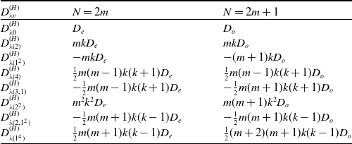
Therefore,

(3.15) \begin{equation} \begin{split} \mathbb{E}^{(H)}_N\left[\det(t-M)^{2k}\right] =& \sum_{\nu\subseteq\lambda}\left(\!-\frac{1}{2N}\right)^{\frac{|\lambda|-|\nu|}{2}}\frac{\text{dim}\, V_\nu}{|\nu|!}t^{|\nu|}\,\text{poly}_{\frac{|\nu|}{2}}(N,k)\\ &\times \begin{cases} C_\lambda(2k) D_e,\quad \text{N even},\\ \\[-8pt] C_\lambda(2k)D_o,\quad \text{N odd}, \end{cases} \end{split} \end{equation}

where $\text{poly}_{j}(N,k)$ denotes a polynomial of degree j in the variables N, k, and the explicit expressions are given in Table 1 for $j\leq 4$ . By referring to (3.10), it is interesting to see that the universal constant $\gamma_k$ is a factor of the moments for any finite N. The first few terms in the moments of characteristic polynomials are

(3.16) \begin{equation}\begin{split}\mathbb{E}^{(H)}_N[\det(t-M)^{2k}]&=\left(\!-\frac{1}{2N}\right)^{Nk}C_\lambda(2k)D_e\\ \\[-8pt]&\quad\times \left[1 + \left(\frac{2^2N^2}{4!}\right)Nk\,t^4 + \left(\frac{2^3N^3}{6!}\right)2Nk(2k-N)t^6 \right.\\ \\[-8pt]&\qquad\left. +\left(\frac{2^4N^4}{8!}\right)Nk (4 N^2 - 17 Nk + 16 k^2+2)t^8 \right.\\ \\[-8pt]&\qquad\left.+ O(t^{10}) \right],\qquad\qquad\qquad\qquad\qquad\qquad\qquad\qquad \text{N even},\\ \\[-8pt]\mathbb{E}^{(H)}_N[\det(t-M)^{2k}]&=\left(\!-\frac{1}{2N}\right)^{Nk}C_\lambda(2k)D_o\left[1 +\left(\frac{2N}{2!}\right)kt^2 +\left(\frac{2^2N^2}{4!}\right)(k^2-Nk)\,t^4\right.\\ \\[-8pt]&\quad\left. + \left(\frac{2^3N^3}{6!}\right)k(2N^2-3Nk+k^2)t^6 \right.\\ \\[-8pt]&\quad\left. +\left(\frac{2^4N^4}{8!}\right)k (\!- 4 N^3+ 15 N^2k - 6 N k^2 -2N+ k^3-4k)t^8\right.\\ \\[-8pt]&\quad\left. +\,\, O(t^{10}) \right],\quad\qquad\qquad\qquad\qquad\qquad\qquad\qquad\qquad \text{N odd}.\end{split}\end{equation}

Up to a factor of $(\!-1)^k$ , both $C_\lambda D_e$ and $C_\lambda D_o$ have the same leading term,

(3.17) \begin{equation}e^{-Nk}(2N)^{Nk+k^2}\gamma_p,\end{equation}

but they differ at sub-leading order as shown in (3.12). In Appendix A, we give the expansion of $C_\lambda(N)D_e$ and $C_\lambda(N)D_o$ up to $O(N^{-6})$ . Note that the fact that the coefficients are polynomial functions of N means that the radius of convergence of the expansion shrinks as $N\to\infty$ . This means that for $t\ne 0$ we cannot use this expansion straightforwardly to determine the large-N asymptotics.

3.2.1 Second moment

The correlations of characteristic polynomials are connected to the correlation functions of random matrices [Reference Mehta40, Reference Forrester20, Reference Mezzadri, Snaith and Hitchin41]. In particular,

(3.18) \begin{equation}R^{(N)}_1(t) = \frac{N!}{(N-1)!}\frac{\mathscr{Z}^{(H)}_{N-1}}{\mathscr{Z}^{(H)}_N}\exp\left(\!-\frac{N t^2}{2}\right)\mathbb{E}^{(H)}_{N-1}\left[\det(t-M)^{2}\right],\end{equation}

where $R^{(N)}_1$ is the one-point density of eigenvalues of matrix size N. As the second moment of the characteristic polynomial is related to the density of states, it is natural to expect the semi-circle law in the limit $N\rightarrow\infty$ as given in (3.1) for a fixed t inside the support of the spectrum. Re-writing (3.1) for $k=1$ ,

(3.19) \begin{equation}\lim_{N\rightarrow\infty}\frac{1}{2N}e^{N\left(1-\frac{ t^2}{2}\right)}\mathbb{E}^{(H)}_{N}\left[\det(t-M)^{2}\right] = \pi\rho_{sc}(t),\end{equation}

which as an expansion in t reads

(3.20) \begin{equation}\lim_{N\rightarrow\infty}\frac{1}{2N}e^{N\left(1-\frac{ t^2}{2}\right)}\mathbb{E}^{(H)}_{N}\left[\det(t-M)^{2}\right] = 1 - \frac{1}{8}t^2 - \frac{1}{128}t^4 - \frac{1}{1024}t^6 + O(t^8).\end{equation}

We now make an observation that we consider surprising: for $k=1$ , starting with (3.14) there is a formal procedure that leads to (3.20). Inserting the asymptotics of $C_\lambda D_e$ and $C_\lambda D_o$ in (3.16), one obtains

(3.21) \begin{align}&e^{-\frac{N t^2}{2}}\mathbb{E}^{(H)}_{N}\left[\det(t-M)^{2}\right] \nonumber\\&= 2Ne^{-N}\bigg[1+\left(\!-\frac{1}{2}N-\frac{5}{12}+O(N^{-1})\right)t^2+\left(\frac{1}{6}N^3 +\frac{19}{72}N^2+\frac{17}{216}N-\frac{811}{77,760}+O(N^{-1})\right)t^4 \nonumber\\&\qquad+\left(\!-\frac{1}{45}N^5-\frac{31}{540}N^4-\frac{323}{6480}N^3-\frac{3667}{291,600}N^2+\frac{799}{1,749,600}N-\frac{640,879}{587,865,600}+ O(N^{-1})\right)t^6 \nonumber\\&\qquad +O(N^{7})O(t^8)\bigg],\quad\text{N even}, \nonumber\\&e^{-\frac{N t^2}{2}}\mathbb{E}^{(H)}_{N}\left[\det(t-M)^{2}\right] \nonumber\\&= 2Ne^{-N}\bigg[1+\left(\frac{1}{2}N+\frac{1}{6}+O(N^{-1})\right)t^2+\left(\!-\frac{1}{6}N^3-\frac{19}{72}N^2-\frac{17}{216}N-\frac{101}{19,440}+O(N^{-1})\right)t^4 \nonumber\\&\quad +\left(\frac{1}{45}N^5+\frac{31}{540}N^4+\frac{323}{6480}N^3+\frac{3667}{291,600}N^2-\frac{799}{1,749,600}N-\frac{15,853}{18,370,800}+O(N^{-1})\right)t^6 \nonumber\\&\qquad +O(N^{7})O(t^8)\bigg],\quad\text{N odd}.\end{align}

Treating the above expansions as a formal series in N and taking their average gives (3.20). In Appendix B, it is shown that the average over even and odd N coincides with the semi-circle law up to $O(t^{10})$ . Also, a general expression for the coefficient of $t^{2j}$ in (3.14) is given for $k=1$ .

Remark 1. For a fixed j, notice that the leading order terms in the coefficients of $t^{2j}$ , which depend on N, differ only by a sign for N even and odd. Therefore, after a formal average of both the series in (3.21), the coefficient of $t^{2j}$ is equal to $c_{2j}+O(N^{-1})$ . The constant $c_{2j}$ turns out to be the appropriate coefficient of $t^{2j}$ in the semi-circle law.

Remark 2. The behaviour exhibited by (3.21) can be understood by considering Figure 1. For a fixed N, the plot shows the behaviour of

(3.22) \begin{equation}f(N,t)=\frac{1}{2N}e^{N\left(1-\frac{ t^2}{2}\right)}\mathbb{E}^{(H)}_{N}\left[\det(t-M)^{2}\right]\end{equation}

as a function of t. The function f(N,t) is oscillatory. The magnitude of the oscillations decreases as N increases, but their length-scale decreases. Moreover, the peaks and troughs of f(N,t) for N even coincides with the troughs and peaks of N odd, respectively. For a fixed j, this explains the divergent polynomial part of N in the coefficients of $t^{2j}$ and the sign change of leading order terms in the N even and odd cases. Formally averaging the two series of f(N,t) when N is even and odd cancels out these oscillations and leaves a result that converges to the semi-circle law.

Figure 1. We plot in (a) f(N,t), defined in (3.22), as a function of t when t is close to the origin for $N=50,\, 51$ ; (b) denotes the same for $N=150,\, 151$ .

Remark 3. As discussed, the size of oscillations in f(N,t) decreases as N increases. Therefore, f(N,t) converges to the semi-circle law as $N\to\infty$ independent of whether N is even or odd. But, at finite but large N, the average of f(N,t) between two consecutive integers is a significantly smoother approximation to the semi-circle law.

3.2.2 Higher moments

For higher moments, the correlations of characteristic polynomials are related to the correlation functions of eigenvalues as

(3.23) \begin{equation}R^{(N)}_k(t_1,\dots,t_k) = \frac{N!}{(N-k)!}\frac{\mathscr{Z}^{(H)}_{N-k}}{\mathscr{Z}^{(H)}_N}\exp\left(\!-\frac{N}{2}\sum_{j=1}^k t_j^2\right)\Delta^2(t_1,\dots,t_k)\mathbb{E}^{(H)}_{N-k}\left[\prod_{j=1}^k\det(t_j-M)^{2}\right],\end{equation}

where $R^{(N)}_k(t_1,\dots,t_k)$ denotes a $k-$ point correlation function of a GUE matrix of size N. The correlations of characteristic polynomials of matrices of size $N-k$ are related to the correlation functions of eigenvalues of matrices of size N. The Dyson sine-kernel for the $k-$ point correlation function and (3.1) for the moments of characteristic polynomials are recovered in the Dyson limit: $t_i-t_j\rightarrow 0$ , $N\rightarrow\infty$ and $N(t_i-t_j)$ is kept finite when $|t_j|<2$ , $j=1,\dots,k$ .

In terms of the Schur polynomials, $\lambda=(N^{2k})$ ,

(3.24) \begin{equation}\mathbb{E}^{(H)}_N\left[\prod_{j=1}^{2k}\det(t_j-M)\right]=C_{\lambda}(2k) \sum_{\nu\subseteq\lambda}\left(\!-\frac{1}{2N}\right)^{\frac{|\lambda|-|\nu|}{2}}\frac{1}{C_\nu(2k)}D^{(H)}_{\lambda \nu}S_\nu(t_1,\dots,t_{2k}).\end{equation}

Computing the asymptotics of moments of characteristic polynomials in the Dyson limit using (3.24) is highly non-trivial. Instead, we fix $t_j=t$ , $j=1,\dots, 2k$ , and give an expansion of the moments as a function of t in the large N limit.

As $N\rightarrow\infty$ , up to $O(t^2)$ ,

(3.25) \begin{equation}\begin{split}&\mathbb{E}^{(H)}_N\left[\det(t-M)^{2k}\right] = (2N)^{k^2}e^{-Nk}\gamma_k\left[1 + O(N^3)O(t^4)\right],\qquad\qquad\qquad\qquad\qquad\quad\,\, N\,\,\text{even}\\&\mathbb{E}^{(H)}_N\left[\det(t-M)^{2k}\right] = (2N)^{k^2}e^{-Nk}\gamma_k\\&\qquad\qquad\qquad\qquad\quad\times \left[1 + t^2\left(Nk+\frac{k^2}{3}(2k^2-1) + O(N^{-1})\right) + O(N^3)O(t^4)\right],\quad N\,\,\text{odd}.\end{split}\end{equation}

Note that the coefficient of $t^2$ is identically zero for even N, where as for odd N it is a polynomial in N and k. Treating the above expansions as a formal series in N and t and taking their average gives

(3.26) \begin{equation}(2N)^{k^2}e^{-Nk}\gamma_k\left(1 + \frac{Nkt^2}{2} +O(N^{2})O(t^4)\right)\left(1 - \frac{k^2t^2}{8}+O(t^{4})\right)\left(1 + \frac{k}{12N}(8k^2-1)+O(N^{-2})\right).\end{equation}

By comparing with (3.1), the terms in the first and second parenthesis of (3.26) are the expansions of $e^{\frac{Nkt^2}{2}}$ and $\pi\rho_{sc}(t)$ up to $O(t^2)$ , respectively.

Similarly, as $N\rightarrow\infty$ , up to $O(t^4)$ ,

(3.27) \begin{equation}\begin{split}\mathbb{E}^{(H)}_N\left[\det(t-M)^{2k}\right] &= (2N)^{k^2}e^{-Nk}\gamma_k\left[1 + t^4\frac{N^3k}{6}\Big(1+\frac{k}{6N}(4k^2+1) \right.\\[3pt]&\qquad \left. + \frac{k^2}{72N^2}(16k^4-16k^2-11)+\frac{k}{6480N^3}(320k^8-1200k^6 \right.\\[3pt]&\qquad \left. +708k^4+1265k^2-756)+O(N^{-4})\Big) + O(N^{5}) O(t^{6})\right],\qquad\qquad\qquad\,\, \text{N even},\\[3pt]\mathbb{E}^{(H)}_N\left[\det(t-M)^{2k}\right] &= (2N)^{k^2}e^{-Nk}\gamma_k\left[1 + t^2\left(Nk+\frac{k^2}{3}(2k^2-1) +O(N^{-1})\right)\right.\\&\qquad\left. + t^4\frac{N^3k}{6}\Big(\!-1 - \frac{2k}{3N}(k^2-2) -\frac{k^2}{18N^2}(4k^4-22k^2+13)\right.\\&\qquad\left. -\frac{k}{405N^3}(20k^8-210k^6+483k^4-385k^2+54)+O(N^{-4})\Big) \right.\\&\qquad\left. +O(N^{5})O(t^6)\right],\qquad\qquad\qquad\qquad\qquad\qquad\qquad\qquad\qquad\qquad\qquad N\,\,\text{odd}.\end{split}\end{equation}

Taking average of the above series and factorising gives

(3.28) \begin{equation}\begin{split}&(2N)^{k^2}e^{-Nk}\gamma_k\left(1 + \frac{Nkt^2}{2} + \frac{N^2k^2t^4}{8} + O(N^{3})O(t^6)\right)\left(1 - \frac{k^2t^2}{8} + \frac{t^4}{128}k^2(k^2-2) + O(t^6)\right)\\&\times\left[1 + \frac{1}{N}\left(\frac{k}{12}(8k^2-1) + \frac{kt^2}{96}(13k^2-1)+O(t^4)\right) + \frac{1}{N^2}\left(\frac{k^2}{144}(32k^4 - 56k^2 + 17) + O(t^2)\right)\right.\\&\left. +O(N^{-3})\right],\end{split}\end{equation}

where the first two brackets correspond to the expansion of $e^{\frac{Nkt^2}{2}}$ and $\pi\rho_{sc}(t)$ , respectively, up to $O(t^4)$ , and the last factor is sub-leading.

4. Secular coefficients

Consider a matrix M of size N. Its characteristic polynomial can be expanded as

(4.1) \begin{equation}\det(t-M)=\prod_{j=1}^N(t-x_j) = \sum_{j=0}^N(\!-1)^{j}\textrm{Sc}_j(M)t^{N-j},\end{equation}

where $\textrm{Sc}_j$ is the $j\textrm{th}$ secular coefficient of the characteristic polynomial. We have

(4.2) \begin{equation}\textrm{Sc}_1(M) = \textrm{Tr} M,\quad \textrm{Sc}_N(M) = \det(M).\end{equation}

These secular coefficients are nothing but the elementary symmetric polynomials $e_j$ defined as

(4.3) \begin{equation}e_j(x_1,\dots,x_N) = \sum_{1\leq k_1<k_2<\dots <k_j\leq N}x_{k_1}x_{k_2}\dots x_{k_j}\end{equation}

for $j\leq N$ and $e_j=0$ for $j>N$ .

The correlations of secular coefficients and their connections to combinatorics have been studied previously [Reference Forrester and Gamburd21, Reference Diaconis and Gamburd17]. For example, the joint moments of secular coefficients of the unitary group are connected to the enumeration of magic squares: matrices with positive entries with prescribed row and column sum. In a similar way, the joint moments of secular coefficients of Hermitian ensembles, such as the GUE, are connected to matching polynomials of closed graphs. In this section, we compute these correlations and indicate their combinatorial properties.

Gaussian ensemble: Elementary symmetric polynomials can be expanded in terms of multivariate Hermite polynomials as

(4.4) \begin{equation}e_r = \sum_{j=0}^{\lfloor\frac{r}{2}\rfloor}\Psi^{(H)}_{(1^r)(1^{r-2j})}\mathscr{H}_{(1^{r-2j})},\end{equation}

where

(4.5) \begin{equation}\Psi^{(H)}_{(1^r)(1^{r-2j})} = (\!-1)^j\frac{(N-r+2j)!}{(2N)^jj!(N-r)!}.\end{equation}

Equivalently, we have

(4.6) \begin{equation}\begin{split}e_{2r} = \sum_{j=0}^r\Psi^{(H)}_{(1^{2r})(1^{2j})}\mathscr{H}_{(1^{2j})},\quad e_{2r+1} = \sum_{j=0}^r\Psi^{(H)}_{(1^{2r+1})(1^{2j+1})}\mathscr{H}_{(1^{2j+1})},\end{split}\end{equation}

with

(4.7) \begin{equation}\begin{split}\Psi^{(H)}_{(1^{2r})(1^{2j})} &= (\!-1)^{r-j}\frac{1}{(2N)^{r-j}(r-j)!}\frac{(N-2j)!}{(N-2r)!},\\ \\[-8pt]\Psi^{(H)}_{(1^{2r+1})(1^{2j+1})} &= (\!-1)^{r-j}\frac{1}{(2N)^{r-j}(r-j)!}\frac{(N-2j-1)!}{(N-2r-1)!}.\end{split}\end{equation}

Because of the orthogonality of the $\mathcal{H}_\mu$ ,

(4.8) \begin{equation}\mathbb{E}^{(H)}_N[\textrm{Sc}_r] = \mathbb{E}^{(H)}_N[e_r] =\begin{cases}(\!-1)^{\dfrac{r}{2}}\frac{1}{(2N)^{\frac{r}{2}}\frac{r}{2}!}\frac{N!}{(N-r)!},& \text{if r is even},\\ \\[-8pt]0,& \text{if r is odd}.\end{cases}\end{equation}

These expectations are nothing but the coefficients of Hermite polynomial of degree N. Thus,

(4.9) \begin{equation}\begin{split}\mathbb{E}^{(H)}_N[\det(t-M)] &= \sum_{j=0}^{\lfloor\frac{N}{2}\rfloor}\mathbb{E}^{(H)}_N[\textrm{Sc}_{2j}(M)]t^{N-2j}=h_N(t),\end{split}\end{equation}

which coincides with (2.20) for $p=1$ . The expectation $|N^j\mathbb{E}^{(H)}_N[\textrm{Sc}_{2j}(M)]|$ is equal to the number of 2j matchings in the complete graph [Reference Diaconis and Gamburd17, Reference Forrester and Gamburd21].

By using (4.4), the second moment of the secular coefficient can also be computed. Similar to the univariate case, multivariate Hermite polynomials $\mathscr{H}_\lambda$ corresponding to even and odd $|\lambda|$ do not mix. Hence, we obtain

(4.10) \begin{equation}\mathbb{E}^{(H)}_N[\textrm{Sc}_{2j}(M)\textrm{Sc}_{2k+1}(M)] = 0,\end{equation}

and

(4.11) \begin{equation}\begin{split}\mathbb{E}^{(H)}_N[\textrm{Sc}_{2r}(M)\textrm{Sc}_{2s}(M)] &= \sum_{j=0}^r\sum_{k=0}^s\Psi^{(H)}_{(1^{2r})(1^{2j})}\Psi^{(H)}_{(1^{2s})(1^{2k})}\mathbb{E}^{(H)}_N[\mathscr{H}_{(1^{2j})}\mathscr{H}_{(1^{2k})}]\\&= \sum_{j=0}^{\min(r,s)}\frac{1}{N^{2j}}\Psi^{(H)}_{(1^{2r})(1^{2j})}\Psi^{(H)}_{(1^{2s})(1^{2j})}C_{(1^{2j})}(N)\\&=\left(\!-\frac{1}{2N}\right)^{r+s}\, \sum_{j=0}^{\min(r,s)}\frac{2^{2j}}{(r-j)!(s-j)!}\frac{N!(N-2j)!}{(N-2r)!(N-2s)!}.\end{split}\end{equation}

Similarly, we write

(4.12) \begin{equation}\mathbb{E}^{(H)}_N[\textrm{Sc}_{2r+1}(M)\textrm{Sc}_{2s+1}(M)] = \left(\!-\frac{1}{2N}\right)^{r+s}\,\sum_{j=0}^{\min(r,s)}\frac{2^{2j}}{(r-j)!(s-j)!}\frac{(N-1)!(N-2j-1)!}{(N-2r-1)!(N-2s-1)!}.\end{equation}

Computing higher order correlations requires evaluating integrals involving a sequence of multivariate Hermite polynomials. Busbridge [Reference Busbridge11, Reference Busbridge12] calculated these integrals for the univariate case, but the results are still unknown for the multivariate generalisation. Instead, we take a different approach by first expressing the product $\prod_j\textrm{Sc}_j(M))^{b_j}$ in terms of the $\mathscr{H}_\mu$ and then using orthogonality for the $\mathscr{H}_\mu$ .

Proposition 4.1. Consider a partition $\lambda = (\lambda_1,\dots ,\lambda_l)$ . We have

(4.13) \begin{equation}\mathbb{E}^{(H)}_N\big[\prod_{j=1}^l\textrm{Sc}_{\lambda_j}(M)\big] =\begin{cases}\sum_\mu \dfrac{1}{(2N)^{\frac{\mu}{2}}\frac{|\mu|}{2}!}K_{\lambda^\prime\mu}\chi^{\mu}_{(2^{|\mu|/2})}C_\mu(N),&\quad \text{if $|\lambda|$ is even},\\ \\[-9pt] 0, &\quad \text{otherwise}.\end{cases}\end{equation}

Here $K_{\lambda\mu}$ are Kostka numbersFootnote 1 and $\chi^\mu_\nu$ is the character of the symmetric group.

Proof. For a partition $\lambda$ , denote

(4.14) \begin{equation}e_\lambda = e_{\lambda_1}e_{\lambda_2}\dots.\end{equation}

Elementary symmetric polynomials $e_\lambda$ can be expanded in Schur basis as follows:

(4.15) \begin{equation}e_\lambda = \sum_{\mu}K_{\lambda^\prime \mu}S_\mu,\end{equation}

where $K_{\lambda\mu}$ are the Kostka numbers [Reference Macdonald39] and $\mu$ is a partition of $|\lambda|$ . Using (2.5),

(4.16) \begin{equation}e_\lambda = \sum_{\mu\vdash |\lambda|}\sum_{\nu\subseteq\mu}K_{\lambda^\prime\mu}\Psi^{(H)}_{\mu\nu}\mathscr{H}_\nu.\end{equation}

When $|\lambda|$ is odd, $\mathbb{E}^{(H)}_N[e_\lambda]=0$ due to the orthogonality of multivariate Hermite polynomials. When $|\lambda|$ is even,

(4.17) \begin{equation}\begin{split}\mathbb{E}^{(H)}_N[e_\lambda] &= \mathbb{E}^{(H)}_N\big[\prod_{j=1}^l\textrm{Sc}_{\lambda_j}(M)\big]\\ &= \mathbb{E}^{(H)}_N\big[\sum_{\mu}\sum_\nu K_{\lambda^\prime\mu}\Psi^{(H)}_{\mu \nu}\mathscr{H}_\nu\big]\\ &=K_{\lambda^\prime\mu}\Psi^{(H)}_{\mu 0}.\end{split}\end{equation}

It can be shown that [Reference Jonnadula, Keating and Mezzadri34]

(4.18) \begin{equation}\Psi^{(H)}_{\mu 0} = \frac{1}{(2N)^{\frac{\mu}{2}}\frac{|\mu|}{2}!}\chi^{\mu}_{(2^{|\mu|/2})}C_\mu(N).\end{equation}

Putting everything together completes the proof.

Laguerre ensemble: All the calculations discussed for the Gaussian ensemble can be extended to the Laguerre and the Jacobi ensembles.

The polynomials $e_r$ can be expanded as

(4.19) \begin{equation}e_r = \sum_{j=0}^{r}\Psi^{(L)}_{(1^r)(1^{j})}\mathscr{L}^{(\gamma)}_{(1^{j})},\end{equation}

where

(4.20) \begin{equation}\Psi^{(L)}_{(1^r)(1^{j})} = \frac{1}{(2N)^{r-j}}\frac{1}{(r-j)!}\frac{(N-j)!}{(N-r)!}\frac{\Gamma(N-j+\gamma +1)}{\Gamma(N-r+\gamma + 1)}.\end{equation}

By using the orthogonality of the multivariate Laguerre polynomials we arrive at

(4.21) \begin{equation}\mathbb{E}^{(L)}_N[\textrm{Sc}_r] = \mathbb{E}^{(L)}_N[e_r] = \frac{1}{(2N)^r}\frac{1}{r!}\frac{N!}{(N-r)!}\frac{\Gamma(N+\gamma +1)}{\Gamma(N-r+\gamma + 1)},\end{equation}

which are the absolute values of the coefficients of the Laguerre polynomial of degree N. For the characteristic polynomial, we have

(4.22) \begin{equation}\mathbb{E}^{(L)}_N[\det(t-M)] = \sum_{j=0}^N(\!-1)^j\mathbb{E}^{(L)}_N[\textrm{Sc}_j(M)]t^{N-j} = l_N^{(\gamma)}(t).\end{equation}

The correlations of secular coefficients can be computed similar to the Gaussian case.

Proposition 4.2. Let $\lambda = (\lambda_1,\dots ,\lambda_l)$ , we have

(4.23) \begin{equation}\mathbb{E}^{(L)}_N\big[\prod_{j=1}^l\textrm{Sc}_{\lambda_j}(M)\big] =\sum_{\mu\vdash |\lambda|}\frac{1}{(2N)^{|\lambda|}}\frac{G_\mu(N,\gamma)G_\mu(N,0)}{G_0(N,\gamma)G_0(N,0)}\frac{\chi^\mu_{(1^{|\mu|})}}{|\lambda|!} K_{\lambda^\prime\mu}.\end{equation}

Proof. The proof is similar to the Gaussian case. By writing

(4.24) \begin{equation}e_\lambda = \sum_\mu\sum_{\nu\subseteq |\lambda|} K_{\lambda^\prime\mu}\Psi^{(L)}_{\mu\nu}\mathscr{L}^{(\gamma)}_\nu,\end{equation}

and using the orthogonality of the multivariate Laguerre polynomials along with the result [Reference Jonnadula, Keating and Mezzadri34]

(4.25) \begin{equation}\Psi^{(L)}_{\mu 0} = \frac{1}{(2N)^{|\mu|}}\frac{G_\mu(N,\gamma)G_\mu(N,0)}{G_0(N,\gamma)G_0(N,0)}\frac{\chi^\mu_{(1^{|\mu|})}}{|\mu|!}\end{equation}

proves the proposition.

Jacobi ensemble. The $e_r$ can be expanded as

(4.26) \begin{equation}e_r = \sum_{j=0}^{r}\Psi^{(J)}_{(1^r)(1^{j})}\mathscr{J}^{(\gamma_1,\gamma_2)}_{(1^{j})},\end{equation}

where $\Psi^{(J)}_{\lambda\nu}$ is given in (2.8). The expected values of the $e_r$ are related to the coefficients of the Jacobi polynomial of degree N.

(4.27) \begin{equation}\mathbb{E}^{(J)}_N[\det(t-M)] = \sum_{j=0}^{N}(\!-1)^j\mathbb{E}^{(J)}_N[\textrm{Sc}_{j}(M)]t^{N-j}=j^{(\gamma_1,\gamma_2)}_N(t)\end{equation}