2. Follow the gap method

FGM is a safety-based geometric obstacle avoidance algorithm that recurrently leads the robot to the goal point while keeping the robot from colliding with the obstacles. [Reference Sezer and Gokasan28] It selects the gaps with maximum angle size, using the sensory information. FGM is a three-stage algorithm. The first stage is calculating the gap arrays. In this stage, the algorithm uses the current sensory information like the LIDAR sensor to generate a gap array. This array contains information about the size of the existing gaps around the robot in angle form. FGM selects the largest gap at the end of this stage, which is called the gap selection process. FGM calculates the angle to the gap’s center point in the second stage, using specific geometric relations. Finally, in the third stage, FGM calculates the final heading angle ( $\varphi_{final}$ ), using Eq. (1). The weighted function mentioned in Eq. (1) consists of the angle to the largest gap’s center point ( $\varphi_{gap-c}$ ), the angle to the goal point ( $\varphi_{goal}$ ), the distance to the closest obstacle ( $d_{\min}$ ), and a safety factor named alpha ( $\alpha$ ). The alpha parameter’s higher values cause the robot to keep its distance from the obstacles and follow the safe gap’s center. In contrast, alpha’s lower values cause the robot to follow the goal point and get too close to obstacles in some cases. These changes in alpha cause the robot to travel on different trajectories, as shown in Fig. 1. The alpha is a user-defined parameter as it is defined in the original paper. Furthermore, it can be noticed in Fig. 1 that the selection of alpha is entirely free and practical, so to continue, we will select $\alpha$ = 40 in this paper.

Figure 1. Visualization of robot’s different paths based on different values of $\alpha$ .

(1) \begin{equation}\varphi_{final} = \frac{\dfrac {\alpha } {d_{\min}} \varphi_{gap-c} + \varphi_{goal}}{\dfrac {\alpha } {d_{\min}} +1}\end{equation}

The visualization of the available gaps around the robot, the angle to the midpoint of the largest gap, the angle to the final goal, and the FGM’s final heading angle are shown in a robot-obstacle configuration represented in Fig. 2.

Figure 2. Robot-obstacle configuration, obstacles (A, B, and C), gaps ( $G_1$ , $G_2$ ), the midpoint of the widest angular gap ( $M_2$ ), goal point (X), angle to the goal point ( $\varphi_{goal}$ ), final heading angle ( $\varphi_{final}$ ), and angle to the largest gap’s center point ( $\varphi_{gap-c}$ ).

Furthermore, although FGM was selected as the most effective and safest obstacle avoidance method in a study by Zohaib et al., [Reference Zohaib, Pasha, Riaz, Javaid, Ilahi and Khan29] it faces a wide range of inherent drawbacks, including the zigzag and the trajectory length problem which were improved by FGM-I. [Reference Demir and Sezer30] Another con of this method is that FGM puts the robot at risk and causes some safety problems using the simple gap selection and final heading angle calculation procedures simultaneously. The next part of this study will cover this drawback in detail and provide a solution by proposing FOCM.

3. Follow the obstacle circle method

FGM is developed to keep the robot safe during travel. This method’s primary part is calculating the final heading angle based on the angle to the gap’s center. In the gap selection stage, the method selects the desired gap by comparing the gaps based on their size in angle, and it does not consider the gaps’ width (in the distance). Although comparing the gaps using the angles is practical, in some cases, it makes the robot travel on unsafe trajectories. An example of this configuration can be seen in Fig. 3, where the FGM puts the robot in a perilous path by selecting the largest gap (G2) among the other available gaps. As shown in Fig. 3, the robot gets too close to obstacle B compared to the safer path shown in green color. This inherent problem cannot be solved by just modifying the FGM’s gap selection procedure because regardless of which gap has been selected, FGM calculates the angle to the gaps’ center point, and the robot has to navigate to that center point straightforwardly for crossing the gap. In other words, FGM uses the heading lines, which start from the robot’s current position and end on the gaps’ center points, so it is possible for the robot to get close to the obstacles during the travel, and in some configuration puts the robot in the risk by getting it too close to the obstacles as shown in Fig. 4. As it is seen in Fig. 4, the shortest distances between the first path, which is created by selecting the largest gap, and the obstacles A and B are $BM_1 = AM_1 = 2$ m. However, the shortest distances between the second path, which is caused by selecting the gap with the largest width, and the obstacles are ( 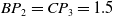$BP_2 = CP_3 = 1.5$ m), so selecting the gap with the largest width does not always lead the robot to safer trajectories when using the FGM. In addition to what has been stated, the safest and the optimum available path for the robot is represented in green color in Fig. 4. It is noteworthy to consider that FGM does not provide this kind of path. The solution to this problem, regardless of the gap selection procedure, requires changing the gap selection procedure and the whole mechanism of the FGM’s final heading calculation. This solution will result in a safe green path represented in Fig. 4. The newly proposed algorithm uses a new concept named “obstacle circles” to compute the final heading angle. Moreover, using this approach allows the robot to travel on safer trajectories using the same sensory information.

Figure 3. Robot-obstacle configuration, where selecting the largest gap by FGM causes the unsafe path in red color. A, B, and C are the obstacles. $M_1$ , $M_2$ are the center of the $G_1$ and $G_2$ gaps, respectively, and the goal point is represented by (X).

Figure 4. The problem of unsafe paths cannot be solved by only modifying the gap selection procedure of FGM.

The freshly proposed algorithm, similar to the FGM, is a three-phase procedure, represented in Fig. 5. The gap selection procedure is explained in Section 3.1. The target heading angle calculation is covered in Section 3.2, and finally, the final heading angle calculation is explained in Section 3.3. At the end of this section, a summary of the algorithm is presented in Section 3.4.

Figure 5. Outline of the newly proposed algorithm.

3.2. Calculation of avoidance heading angle for each gap

Irrespective of the chosen gap, a robot must cross the gap baseline (the segment connecting the obstacle borders to each other). Selecting the gaps’ centers is mathematically optimal for passing the robot through the gap baseline because the robot will have the maximum distance from obstacles there. Considering the fact that the robot will have this distance in the best situation will lead us to use the mentioned distance as a margin between the robot and obstacles, where this margin is a locus of points equidistant from obstacles in 2D that creates “obstacle circles” with the radius of the minimum distance from the obstacles to the center of each gap baseline. We will call this radius as gap radius ( $r_{gap}$ ). Considering the robot-obstacle configuration scenario shown in Fig. 6, the obstacle circles are notable in each gap. It is noteworthy to mention that the center of these obstacle circles are gap borders (the edges of obstacles); these centers can be calculated by obtaining the distance and the angle information from the robot to the obstacles’ edges (gap borders) using the sensory data. The calculation contains scanning the LIDAR data continuously and detecting the obstacle edges then converting the polar coordinates of obstacle borders to the Cartesian coordinate systems. Figure 7 represents an actual scene of the robot-obstacle configuration, and visualization of robot, the obstacle (box in black), LIDAR data in red, robot’s LIDAR range (representing LIDAR field of view [FOV]), first gap (G1 in green), second gap (G2 in gold), center of obstacle circles (OC11 and OC12 for the first gap; OC21 and OC22 for the second gap), obstacle circles for each gap, and distance from robot to the center of obstacle circles (d1 and d2).

Figure 6. Obstacle circles for the obstacles A, B, and C.

Figure 7. Visualization of the robot-obstacle configuration, where it shows: robot, obstacle (box in black), LIDAR data in red, robot’s LIDAR range in blue (representing the LIDAR FOV), first gap (G1 in green), second gap (G2 in gold), center of obstacle circles (OC11 and OC12 for the first gap; OC21 and OC22 for the second gap), obstacle circles for each gap, and distance from robot to the center of obstacle circles (d1 and d2).

Following the obstacle circle with the largest radius will guarantee the robot’s safety during the travel because it would have the most considerable maximum distance to obstacles among the other gaps, not only on the gap baseline but also everywhere on the robot-obstacles configuration. Figure 8 demonstrates the possible path that tracks the obstacle circle without getting inside the circle (Path 1) and the path created by FGM (Path 2). It is evident that by considering the mentioned obstacle circles instead of the FGM’s gap center angle, the new algorithm drives the robot to safer trajectories by keeping the robot out of the dangerous zone. The shortest path that a robot can travel with the constraint of ( $d_{\min} \geq r_{gap}$ ), is Path 1, which is represented in blue color in Fig. 6, where $d_{\min}$ is the shortest distance from the robot to the obstacles in the selected gap. The calculation of Path 1 depends on the robot’s position regarding the obstacle circles, whether the robot is inside/on the obstacle circle or outside the obstacle circle. The proposed algorithm compares the minimum distance between the robot and obstacles and the gap radius ( $r_{gap}$ ) for each gap. Consequently, there are two possible cases, as follows:

Figure 8. Demonstrates the possible path that tracks the obstacle circle without getting inside the circle (Path 1) and the path created by FGM.

1- If $d_{\min}$ is more extensive than $r_{gap}$ as shown in Eq. (2), the robot is outside the obstacle circles:

(2) \begin{equation}d_{\min}>r_{gap}\end{equation}

In this case, the robot will try to get itself as close as possible to the gap center with the constraint of ( $d_{\min}>r_{gap}$ ). To make this maneuver possible, the algorithm calculates a heading angle named as “avoidance heading angle” ( $\varphi_{Avoid}$ ) to the best tangent point on the closest obstacle circles. It considers the distance to the center of each obstacle circle (finding the closest circle – discarding two tangent points out of four) and then compares the angle between the robot, the gap’s center point, and two tangent points. Then it selects the minimum one to find the best tangent. Figure 9 demonstrates the flowchart used for selecting the best tangent point. Figure 10 represents an example of this procedure for a robot-obstacle configuration. As it is seen in this figure, the algorithm first selects the obstacle circle B as the closest obstacle circle (selecting the tangent points R1 and R2), then it compares the angle between the gap’s center point, the robot, and the tangent points and as a result, selects the R2 as the best tangent point ( $M_2 \hat{R} R_2 < M_2 \hat{R} R_1$ ). Also, it is notable to mention that each tangent point can be calculated by knowing the obstacle circle’s equation (center and radius) and a point outside the circle, which in our case, it is the robot’s position. Figure 11 represents a path traveled by the robot under this circumstance for the robot-obstacle configuration mentioned in Fig. 10.

Figure 9. The flowchart of selecting the best tangent point. $\varphi_{cg}$ is the heading angle from the robot to the center of the gap, $\Theta_{t_1}$ and $\Theta_{t2}$ are the heading angles from the robot to tangent points $\#1$ and $\#2$ .

Figure 10. Robot-obstacles configuration, where the R2 tangent point has been selected as the best tangent point. A, B, and C are the obstacles. $R_1$ , $R_2$ , $L_1$ , $L_2$ are the tangent points. $M_2$ is the center of the largest gap in width.

Figure 11. Visualization of the traveled path of the robot from outside the circle where $d_{\min}$ $>$ $r_{gap}$ .

2- If $d_{\min}$ is smaller than or equal to $r_{gap}$ as shown in Eq. (3), the robot is inside or on the obstacle circles:

(3) \begin{equation}d_{\min}\leq r_{gap}\end{equation}

In this case, the robot, whether on the obstacle circle or inside the circle, can have any heading angle, and its distance to the center of the obstacle circle is at least $d_{\min}$ . In this situation, for considering all possible cases simultaneously, the algorithm creates a virtual circle with the center of the closest obstacle coordinate and the radius of $d_{\min}$ with the same logic used for creating the obstacle circles, which was using the minimum distance from the robot to the obstacles and using this distance as the margin between them. The robot needs to update its heading angle recursively to track this curve, keeping/making itself tangent to the curve. So the algorithm calculates the difference between the robot’s heading angle and the angle of the vector $\vec{T}$ , which is perpendicular to the radius, as shown in Fig. 12(a). This difference angle would be the target heading angle ( $\varphi_{Avoid}$ ) for the robot. Figure 12(b) demonstrates the robot’s traveled path while tracking circular arcs inside the obstacle circle and recursively updating its heading angle in the identical configuration as shown in Fig. 12(a).

Figure 12. (a): Visualization of how the robot tracks a circular arc inside the obstacle circle recursively updating its heading angle. (b): Visualization of the traveled path by the robot while tracking a circular arc, recursively updating its heading angle in the identical configuration as shown in Fig. 10(a).

3.3. Calculation of the final heading angle for each gap

After calculating the avoidance heading angle ( $\varphi_{Avoid}$ ) from the previous steps, the algorithm is now able to calculate the final heading angle. For this step, the algorithm uses the FGM’s final heading angle equation as mentioned in Eq. (1). The only difference is, instead of using the angle to the gaps’ center point, it uses avoidance heading angle ( $\varphi_{Avoid}$ ).

To have a clear vision about the difference between the FGM and the newly proposed algorithm FOCM, the simulation results of two different robot-obstacle configurations containing multiple obstacles are visualized in Fig. 11. As shown in Fig. 13(a), the traveled paths for both FGM and FOCM algorithms from the initial state until the moment where the robot detects the obstacle are identical. After detecting the obstacle, the FOCM forms a proper obstacle circle and passes the obstacle by tracking the circle and keeping its margin ( $r_{gap}$ ) from the obstacle. However, FGM calculates the heading angle to the center of the largest gap instead. As a result, FGM enters the dangerous zone (inside the obstacle circle). Although both algorithms reach the target state, the path caused by FOCM is safer than the path created using the FGM. Figure 13(b) demonstrates a complex robot-obstacle configuration where the newly proposed algorithm was tested multiple times during the travel. As shown in Fig. 13(b), the robot using the FGM entered into the obstacle circles, and consequently, it leads the robot to an unsafe path compared with the FOCM.

Figure 13. Comparison of the FGM and FOCM.

3.4. Algorithm’s summary

FOCM is a practical safety-based obstacle avoidance algorithm. Gap selection and avoidance strategies are improved comparing to FGM. A flowchart is represented in Fig. 14, which demonstrates the summary of the proposed methodology.

Figure 14. The flowchart of the methodology.

4. Simulation results

To have a fair comparison between FOCM and the classical FGM, Monte Carlo simulations are performed. A CAD model of differential drive wheelchair, which is identical to the real autonomous wheelchair used in experimental tests, is prepared as shown in Fig. 15 and is used in simulations. Matlab is used for developing a simulation environment with an area of 7 m $\times$ 14 m. The starting and the final points’ coordinates are chosen as [11.8-13] and [16.5-13], respectively. A LIDAR sensor with a total of 180 degrees FOV is used in the simulations.

Figure 15. Differential drive wheelchair’s CAD model.

To obtain a fair benchmarking, both methods used the identical proportional and integral (PI) heading angle controller during the simulations, and the linear velocity of both methods is selected as constant 0.15 m/s. This value is selected small similar to the output of a fuzzy-logic-based longitudinal velocity planner, mentioned in ref. [Reference Sezer, Ercan, Heceoglu, Bogosyan and Gokasan35]. The mentioned heading angle controller is introduced in Eq. (4):

(4) \begin{equation}w = k_p(\varphi_{final} -\theta_{robot})+k_i\left(\int\!\!\left(\varphi_{final}-\theta_{robot}\right)\!\!\right.dt\end{equation}

Where $\theta_{robot}$ is the robot’s momentary heading angle, and $\varphi_{final}$ is the algorithm’s final guiding angle. $K_p$ and $K_i$ are the PI gains, respectively. These values are tuned empirically by trial and error tests in our previous wheelchair conversion study. [Reference Sezer, Zengin, Houshyari and Yilmaz36] For a fair comparison of FOCM and FGM, same controller coefficient values are used. $K_p$ and $K_i$ are selected as 0.3 and 0.5, respectively. Increasing the values of $K_p$ and $K_i$ decreases the rising time and increases the overshoot, from a classical PI controller design perspective. Although performing an impartial comparison between the two algorithms is challenging, 600 Monte Carlo simulations are performed to compare both methods. In these simulations, the obstacles are spread uniformly where the positions are set randomly. A computer with the 10th generation of i7 4.6 GHz Intel CPU and 16 GB of RAM, operating the Ubuntu 16.04 OS, was used to perform the simulations. To have a clear vision of the proposed algorithm’s efficiency, multiple performance measures such as obstacle avoidance safety metric and the travel’s average length are used. The obstacle avoidance safety metric used in this study is given in Eq. (5) as it is used in ref. [Reference Nair and Kobilarov37]. The p’th norm of any f(t) function can be calculated using Eq. (6):

(5) \begin{equation} f(t) = \left\{ \begin{array}{@{}cclc} \dfrac{1}{d_{\min}}-\dfrac{1}{d_0} &,& \text{for} \: \: \: d_{\min}<d_0\\[10pt]0 &,& \text{for} \: \: \: d_{\min}\geq d_0 \end{array} \right. \end{equation}

(6) \begin{equation}\|f\|_{p}= (|f(t)|^{p}dt)^{1/p}x\end{equation}

where $d_{\min}$ is the shortest distance between the robot and the existing obstacles, and the scalar $d_{0}$ stands for the distance to an obstacle that is not dangerous for the robot. This is a user-defined analysis parameter and considering the indoor environment condition, $d_{0}$ is selected as 2 m. This is a parameter for analysis of the resulting paths in terms of the danger. While increasing $d_{0}$ considers unnecessary distant measurements, decreasing $d_{0}$ ignores critically close obstacles. This value can be higher for outdoor conditions. The mentioned collision avoidance safety metric is inversely proportional to the closest distance between the obstacles and the robot. In other words, it is a penalizing function that penalizes the robot when it gets closer to obstacles than the scalar $d_{0}$ , a smaller average value means a safer travel. Same collision avoidance metric was previously used in refs. [Reference Sezer and Gokasan28, Reference Demir and Sezer30, Reference Houshyari and Sezer34, Reference Nair and Kobilarov37]. Furthermore, in this study, the infinity norm ( $p = \infty$ ) of the obstacle avoidance safety metric is used for comparison.

Table I demonstrates the average of mentioned performance measures for the total 600 Monte Carlo simulations of FGM and FOCM ( $\alpha=40$ , $d_0=2$ m).

Table I. Monte Carlo simulations result ( $\alpha = 40$ )

According to Table I, the newly proposed FOCM is 12.79% safer than the FGM, while the average travel distance values are almost equal. The FOCM average traveled distance is 1.71%, longer than FGM.

In order to test the statistical significance of the algorithm in performing the safety of the obstacle avoidance task, we apply Z test since the sample size (number of simulations: $n=600$ ) is large enough. This allows us to assume that the sampling distribution is approximately normal with the mean of FGM’s safety metric $\mu_{FGM}$ , and its standard deviation of $s=2.732.$ We use the variable Z as the test statistic under the hypothesis represented in Eq. (7):

(7) \begin{equation} \left\{ \begin{array}{l@{\quad}l} H_0,\ \ \mu_{FOCM} \geq \mu_{FGM} & \text{(Null Hypothesis)} \\[10pt] H_1, \ \ \mu_{FOCM} < \mu_{FGM} & \text{(Alternative Hypothesis)} \end{array} \right. \end{equation}

It is noteworthy to mention that the Z value is calculated as $-2.4995$ , using the general Eq. (8), where $\bar{x}$ is the mean score of FOCM’s safety metric ( $\mu_{FOCM} $ ) and $\mu$ is the mean score of the FGM’s safety metric ( $\mu_{FGM} $ ).

(8) \begin{equation}Z = \frac{\bar{x} - \mu}{\dfrac {s} {\sqrt{n}}}\end{equation}

The confidence level is chosen as $c=0.95$ , so the significance level is 0.05 which is a common selection in most of the tests of statistically significance. The critical Z value, which represents the boundary between rejection and acceptance of the null hypothesis $H_{0}$ for the defined significance level, is $-1.96$ . Furthermore, p-value is a number which describes how likely it is that our data would have occurred by random chance under the assumption of null hypothesis is true. In our case, for the calculated Z value $-2.7794$ , p-value is 0.0028. Since the calculated Z value falls outside the critical value which means that the p-value is lower than the defined significance level ( 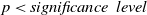$p < significance \: \: level$ ), the $H_{0}$ is successfully rejected. This means that the mean of the safety metric of FOCM is significantly lower than FGM, which shows the safety advantage of FOCM over FGM statistically. Figure 16 represents the normal distribution, Z value, and critical value.

Figure 16. Visualization of the normal distribution, test statistic value, and critical value of left-tail test.

5. Experimental platform

After getting the satisfying results from the simulations, FOCM is implemented on the real autonomous platform to test its real-time performance. The real system used in this study is a fully autonomous electrical wheelchair testbed, which is designed and developed by the Autonomous Mobility Group of Istanbul Technical University [Reference Sezer, Zengin, Houshyari and Yilmaz36]. It is constituted with multiple sensors like three LIDARs, an RGB-D camera, an IMU sensor, and wheel encoders. The computational hardware mounted on this wheelchair includes Nvidia Jetson-TX2 and AAEON Intel Upboard for high-level operations. An embedded ST B-F446E96B01A board is used for low-level control applications. Figure 17 illustrates the wheelchair with its sensors and computational hardware. The autonomous wheelchair uses the robot operating system (ROS) as the central platform for communicating and has the ability to be controlled semi/fully autonomously and manually by an operator. Figure 18 visualizes the communication architecture used for developing this wheelchair. More detailed information about the experimental platform can be found in ref. [Reference Sezer, Zengin, Houshyari and Yilmaz36].

Figure 17. Visualization of fully autonomous wheelchair and its components as an experimental platform.

Figure 18. Visualization of the communication architecture used in the experimental platform.

6. Experimental results

Both FOCM and FGM are coded in Python as independent ROS nodes. The tunable parameter alpha is chosen as 40 ( $\alpha=40$ ) for both methods to have a fair comparison. The wheelchair uses identical PI heading angle controller we used during the simulations. Since the tests are mostly done in challenging environments, the linear velocity of both methods is selected similar to the output of a fuzzy-logic-based longitudinal velocity planner in such complex scenarios. [Reference Sezer, Ercan, Heceoglu, Bogosyan and Gokasan35] The SICK LMS 151 LIDAR is used for perception with a limited FOV of 150° and a limited maximum range of 3 m. The adaptive Monte Carlo localization method [Reference Dellaert, Fox, Burgard and Thrun38] is used for localization during the experimental tests. Figure 19 represents the real occupancy grid map of the Mechatronics Educational and Research Center (MEAM) of Istanbul Technical University, which is chosen as the test field. Four complex scenarios are chosen to perform the tests. The results of the first scenario of experimental tests are represented in Fig. 20. Figure 20(a) shows the initial point of the autonomous wheelchair, the paths created by both FOCM and FGM algorithms, the final point, and the obstacle measurements from the LIDAR sensor. As it can be seen in Fig. 20(b), which is the zoomed version of Fig. 17(a), the wheelchair’s initial coordinate is selected as [8.2,10], and the goal point’s coordinates is [9.1,3]. The path created by FGM is shown in red color, and the traveled path caused by FOCM is represented in blue color. The purple and the green points are the obstacle measurements coming from the LIDAR. The obstacle measurement clusters are not identical because of the noise and the uncertainty that the LIDAR contains during the measurement. Figure 21 shows the sequential recorded images of the wheelchair’s travel during the tests. Figure 21(a) depicts the test using the FGM, whereas Fig. 21(b) illustrates the travel of the wheelchair using the newly purposed FOCM. In order to show the safety effect of the proposed approach, Fig. 22. shows the merged image of both algorithms at the critical moment while overtaking the obstacle. Moreover, the real video of these tests can be watched online by clicking here, or from Supplementary Material part of the submission.

Figure 19. The real occupancy grid map of the test field.

Figure 20. The results of the first scenario of experimental test.

Figure 21. The recorded images of the first scenario of the experimental tests (a): The experimental test using the FGM; (b): The experimental test using the FOCM.

Figure 22. The merged image of both algorithms’ critical moment.

Table II demonstrates the average and the standard deviation of the safety metric for the five tests of FGM and FOCM in the first scenario ( $\alpha=40$ , $d_0=2$ m).

Table II. Experimental results of first scenario ( $\alpha =40$ )

According to the real experimental tests, as shown in Table II, the newly proposed FOCM is 8.6%, safer than FGM, while the average travel distance values are almost equal. The FOCM average traveled distance is 1.57%, longer than FGM.

Figure 23 represents the second scenario of the experimental tests. As it can be seen in Fig. 23(b), which is the zoomed version of Fig. 23(a), the wheelchair’s initial coordinate is selected as [9.8,10], and the goal point’s coordinates is [8.5,3.5]. The path created by FGM is shown in red color, and the traveled path caused by FOCM is represented in blue color. The purple and the green points are the obstacle measurements coming from the LIDAR. Figure 24 illustrates the sequential recorded images of the wheelchair’s travel during the tests. Figure 24(a) depicts the test using the FGM, whereas Fig. 24(b) shows the travel of the wheelchair using the FOCM. Moreover, Table III demonstrates the average and the standard deviation of the safety metric for the five tests of FGM and FOCM in the second scenario.

Figure 23. The results of the second scenario of experimental test.

Figure 24. The recorded images of the second scenario of the experimental tests (a): The experimental test using the FGM; (b): The experimental test using the FOCM.

Table III. Experimental results of second scenario ( $\alpha$ =40)

According to the experimental tests, as shown in Table III, FOCM average traveled distance is 3.1%, longer than FGM, and FOCM is 7.7%, safer than FGM, while the average travel distance values are almost equal.

Figure 25 visualizes the third and the most complex scenario available in the MEAM. As it can be seen in Fig. 25(b), which is the zoomed version of Fig. 25(a), the wheelchair’s initial coordinate is selected as [8.2,10], and the goal point’s coordinates is [9.2,3.2]. Similar to the previous tests, the path created by FGM is shown in red color, and the traveled path caused by FOCM is represented in blue color. The purple and the green points are the obstacle measurements coming from the LIDAR. Figure 26 depicts the sequential recorded images of the wheelchair’s travel during the tests. Figure 26(a) shows the test using the FGM, whereas Fig. 26(b) shows the travel of the wheelchair using the FOCM. Furthermore, Table IV demonstrates the average and the standard deviation of the safety metric for the five tests of FGM and FOCM in the third scenario.

Figure 25. The results of the third scenario of experimental test.

Figure 26. The recorded images of third scenario of the experimental tests (a): The experimental test using the FGM; (b): The experimental test using the FOCM.

Table IV. Experimental results of third scenario ( $\alpha$ =40)

According to Table IV, the mean of traveled distance caused by FOCM is averagely 0.35% longer than FGM; however, FOCM leads the robot to safer trajectories, and it is 14.81% safer than FGM, while the average travel distance values are almost equal.

Finally, comparing the FGM and FOCM with the presence of dynamic obstacles is challenging. It is not realistic to provide the same scenarios (same position, velocity, and heading configuration of dynamic obstacles for same time segments) for both algorithms. On the other hand, in order to show the capability of FOCM to handle the scenarios with the presence of dynamic obstacles, we provided the fourth test scenario represented in Fig. 27. As it can be seen in Fig. 27(b), which is the zoomed version of Fig. 27(a), the wheelchair’s initial coordinate is selected as [9.2,10], and the goal point’s coordinates are [9.0,3.2]. The traveled path caused by FOCM is represented in blue color. The green points are the obstacle measurements coming from the LIDAR. Although the wheelchair’s path and the obstacle measurements seem to intersect, they are not collisions since the robot and the obstacles are at the same place in different times. This can be seen in Fig. 28. which illustrates the sequential recorded images of the wheelchair’s travel during the tests using the FOCM.

Figure 27. The results of the fourth scenario with the presence of the random dynamic obstacles, for showing the capability of FOCM to handle the scenarios with the presence of dynamic obstacles.

Figure 28. The recorded images of the fourth scenario of the experimental tests using FOCM with the presence of random dynamic obstacles.