


1. INTRODUCTION
Over the last two decades, as Greenland's marine-terminating outlet glaciers have retreated, thinned and accelerated, the flux of icebergs to Greenland's fjords and coastal waterways has increased (Bigg and others, Reference Bigg2014). Until recently, these icebergs remained a relatively understudied phenomena despite their physical, ecological and socioeconomic importance. Unlike point sources of freshwater such as meltwater streams, rivers and subglacial conduits, icebergs represent a distributed source of freshwater (Silva and others, Reference Silva, Bigg and Nicholls2006). Depending on where drifting icebergs melt, their freshwater may play an important role in fjord stratification (Sutherland and others, Reference Sutherland2014), overturning circulation (Bamber and others, Reference Bamber, van den Broeke, Ettema, Lenaerts and Rignot2012) and/or ecosystem structure (Greene and others, Reference Greene, Pershing, Cronin and Ceci2008). The physical characteristics of icebergs can provide important insights into the dynamics of the glaciers that produced them (Bassis and Jacobs, Reference Bassis and Jacobs2013), and the number and sizes of icebergs in a fjord or shelf area places a constraint on their potential freshwater flux (Sutherland and others, Reference Sutherland2014; Enderlin and others, Reference Enderlin, Hamilton, Straneo and Sutherland2016; Moon and others, Reference Moon2018). Recent analyses suggest that time series of iceberg melting can be used to infer variations in subsurface ocean conditions and ice-ocean interactions near glacier termini (Enderlin and others, Reference Enderlin2018). Icebergs also pose hazards to marine navigation and offshore infrastructure in the Arctic (e.g. Sackinger and others, Reference Sackinger, Shoemaker, Serson, Jeffries and Van1985; Fuglem and Jordann, Reference Fuglem and Jordann2017), where natural resource exploration and shipping are expanding (Pizzolato and others, Reference Pizzolato, Howell, Derksen, Dawson and Copland2014).
At any given point in time, there may be tens of thousands of icebergs in a fjord or bay (Enderlin and others, Reference Enderlin, Hamilton, Straneo and Sutherland2016), posing a challenge to manual iceberg identification using satellite images. Iceberg detection and size characterization is further hindered by the presence of clouds in visible to near-infrared satellite imagery. Excluding images with partial cloud cover would considerably limit the temporal resolution of any derived dataset, resulting in potential aliasing of changes in iceberg size distributions over time. Therefore, efficient mapping of icebergs mandates that clouds are automatically distinguished from snow and ice in satellite images (i.e. automated cloud masking).
The primary challenge in mapping clouds in satellite images is that clouds and snow/ice share similar spectral properties across a large portion of the electromagnetic spectrum typically sensed by satellite platforms. Clouds and snow/ice are especially similar in the visible wavelengths (highly reflective) and thermal wavelengths (cold), properties that often allow clouds to be readily distinguished from relatively warm and dark-colored land surfaces. Common cloud detection schemes for optical imagery, including a few designed specifically for the Landsat sensors (e.g. Irish and others, Reference Irish, Barker, Goward and Arvidson2006; Oreopoulos and others, Reference Oreopoulos, Wilson and Várnai2011; Kustiyo and others, Reference Kustiyo, Dianovita, Ismaya, Rahayu and Adiningsih2012; Zhu and Woodcock, Reference Zhu and Woodcock2012; Foga and others, Reference Foga2017), use band thresholding, both of individual bands and combinations of bands, to exploit differences in the spectral properties of the different media (e.g. Racoviteanu and others, Reference Racoviteanu, Paul, Raup, Khalsa and Armstrong2009). Often, several thresholding approaches are combined and/or advanced computing and image analysis techniques are utilized to achieve the best results (e.g. Hall and others, Reference Hall, Riggs and Salomonson1995; Riggs and Hall, Reference Riggs and Hall2002; Scaramuzza and others, Reference Scaramuzza, Bouchard and Dwyer2012; Zhu and Woodcock, Reference Zhu and Woodcock2012). However, the existing cloud masking approaches often fail to accurately differentiate clouds from ice and snow surfaces (Oreopoulos and others, Reference Oreopoulos, Wilson and Várnai2011; Foga and others, Reference Foga2017), including or excluding both clouds and snow/ice simultaneously. Dozier (Reference Dozier1989), Riggs and Hall (Reference Riggs and Hall2002), Irish and others (Reference Irish, Barker, Goward and Arvidson2006), Jedlovec (Reference Jedlovec and Jedlovec2009) and many others provide insight on various approaches to generating cloud masks for optical satellite images, including advanced image analysis techniques based on machine learning (Lee and others, Reference Lee, Weger, Sengupta and Welch1990; Scaramuzza and others, Reference Scaramuzza, Bouchard and Dwyer2012; Hughes and Hayes, Reference Hughes and Hayes2014) and edge detection (Zhu and Woodcock, Reference Zhu and Woodcock2012).
To generate a dataset that captures changes in iceberg size distributions, we developed a Landsat-based semi-automated iceberg delineation algorithm that incorporates a machine learning-based cloud mask. We present details of the algorithm and results from Disko Bay, West Greenland, to demonstrate the utility of the algorithm to explore temporal changes in iceberg size distributions commensurate with glacier change. Our method was developed so that it can be implemented locally on a standard computer and with minimal user input, subsequent to the one-time development of appropriate regional input files. We validate our cloud mask through manual analysis and evaluation of model output against a validation dataset for Disko Bay, and iceberg detection is validated using visual inspection and an independent application in Kangerlussuup Sermia Fjord. Finally, we compare changes in iceberg size distributions in Disko Bay between 2000–02 and 2013–15 to explore the use of iceberg size distribution time series as a means to infer changes in glacier dynamics. We find that the ice cover and iceberg size distributions change over time concurrent with a shift in parent glacier calving style.
2. STUDY REGION
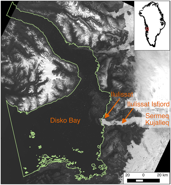
A critical location to study icebergs around Greenland is along the central west coast (Fig. 1). Icebergs transit through the Labrador Sea into the shipping lanes of the North Atlantic (e.g. Bigg and others, Reference Bigg, Wadley, Stevens and Johnson1997), and their meltwater has the potential to disrupt the formation of North Atlantic Deep Water (NADW) (Fichefet and others, Reference Fichefet2003). We chose Disko Bay as our study site due to the pronounced changes in iceberg calving style and volume from the primary iceberg source (Sermeq Kujalleq, or Jakobshavn Isbræ) (e.g. Amundson and others, Reference Amundson2008; Joughin and others, Reference Joughin2008; Cassotto and others, Reference Cassotto, Fahnestock, Amundson, Truffer and Joughin2015, and references therein), the most prolific producer of icebergs in Greenland (Enderlin and others, Reference Enderlin2014), and the importance of icebergs to local communities. Icebergs calve into the deep Ilulissat (Jakobshavn) Isfjord and traverse the ~ 60 km long fjord until it empties into Disko Bay. Changes in the style, and likely size and volume, of icebergs calved from Sermeq Kujalleq initiated in the late 1990s and continued throughout the 2000s as the glacier's terminus retreated and its geometry evolved (Amundson and others, Reference Amundson2008; Joughin and others, Reference Joughin2008).

Fig. 1. Location of Disko Bay, the study region, in West Greenland. Features of note include Sermeq Kujalleq (i.e. the iceberg source), Ilulissat Isfjord, the town of Ilulissat, and the study region of interest (ROI, green outline). Background is a mosaic of Landsat 8 panchromatic images from summer 2015.
North of the fjord mouth, along the eastern shore of the bay, sits the town of Ilulissat. Residents here depend heavily on fishing and tourism, so navigability of Disko Bay's iceberg laden waters is of critical importance to their livelihoods (personal communication from local marine operators, 2014). Anecdotal evidence suggests that the number and size distribution of icebergs present in Disko Bay has changed in recent decades as Sermeq Kujalleq has thinned and retreated. Specifically, marine navigators and fishermen noted that in more recent years, relative to the turn of the century, the bay is frequently covered with a large number of small icebergs, making navigation and fishing difficult (personal communication from local marine operators, 2014). However, to date, there is no comprehensive analysis of temporal variations in iceberg size distributions in Disko Bay.
Automated optical approaches, such as that used below, rely on the contrast between bright iceberg surfaces and the comparatively dark water surrounding them. Thus, they are unable to distinguish individual icebergs that are tightly packed. To avoid problems associated with automated detection of icebergs surrounded by sea/brash ice or dammed by icebergs stranded on the ~200 m deep sill at the mouth of Ilulissat Isfjord, we focused our study during the summer months and on the area seaward of the sill. The exclusion of the fjord mouth enabled us to avoid detections of erroneously large ‘icebergs’ that were actually a combination of multiple icebergs stranded close together.
3. METHODS
3.1. Imagery selection
Given our time period of interest and the relatively small iceberg sizes found in Ilulissat Isfjord (Enderlin and others, Reference Enderlin, Hamilton, Straneo and Sutherland2016), we considered only the Landsat suite of sensors and focused on the derivation of a semi-automated algorithm that works across the archive. Alternative optical and radar imagery resources have relatively coarse spatial resolutions (e.g. minimum of 250 m for MODIS) relative to Landsat (minimum 15 m) or do not cover the time period of dynamic change in Sermeq Kujalleq. Images from 2000 to 2002 were collected by Landsat 7 (ETM+) while images from 2013 to 2015 were collected by Landsat 8 (OLI and TIRS). Both Landsat 7 and 8 have a panchromatic band with 15 m spatial resolution, visible through short-wave infrared (SWIR) bands with 30 m spatial resolution and thermal bands with 60–100 m (Landsat 7 and 8, respectively) spatial resolution. For processing steps that simultaneously utilized multiple bands of different native resolutions, scenes were upsampled to the highest resolution of any of the input bands. For example, the cloud mask was generated at 30 m pixel resolution, then each mask pixel was parsed into four 15 m × 15 m pixels that each have the same value as the parent pixel. The potential impacts of this resampling are discussed below.
We downloaded pre-collection Landsat scenes spanning path numbers 10–11 and row numbers 11–12 from the USGS EarthExplorer website (earthexplorer.usgs.gov). Mosaicking of multiple scenes collected during the same pass maximized coverage. The relatively high latitude of Disko Bay (~68.5°–70° North) provided the advantage of a satellite repeat interval better than the 16 day standard repeat time for Landsat with the concurrent disadvantage of limiting our analysis seasonally. To minimize inclusion of springtime scenes that contained extensive sea ice (Cassotto and others, Reference Cassotto, Fahnestock, Amundson, Truffer and Joughin2015), even during periods of sufficient solar illumination (February–October), we considered only scenes with collection dates from May to October. We manually screened these scenes to exclude from download those with such extensive cloud or sea ice cover that icebergs could not easily be distinguished because this visual inspection takes only 30–60 seconds compared to the ~5 minutes required to generate a cloud mask using our algorithm. We opted for manual screening because the automatically generated percent cloud cover provided with each Landsat scene was an unreliable indicator of the presence of clouds over our marine area of interest. Approximately 70% of the available images contained manually-identifiable icebergs, providing 9–14 (median 10) usable image swaths for a given year.
3.2. Algorithm
A schematic of the procedure to detect icebergs in both cloud-free and partially cloudy Landsat scenes is shown in Fig. 2 and described in detail below.
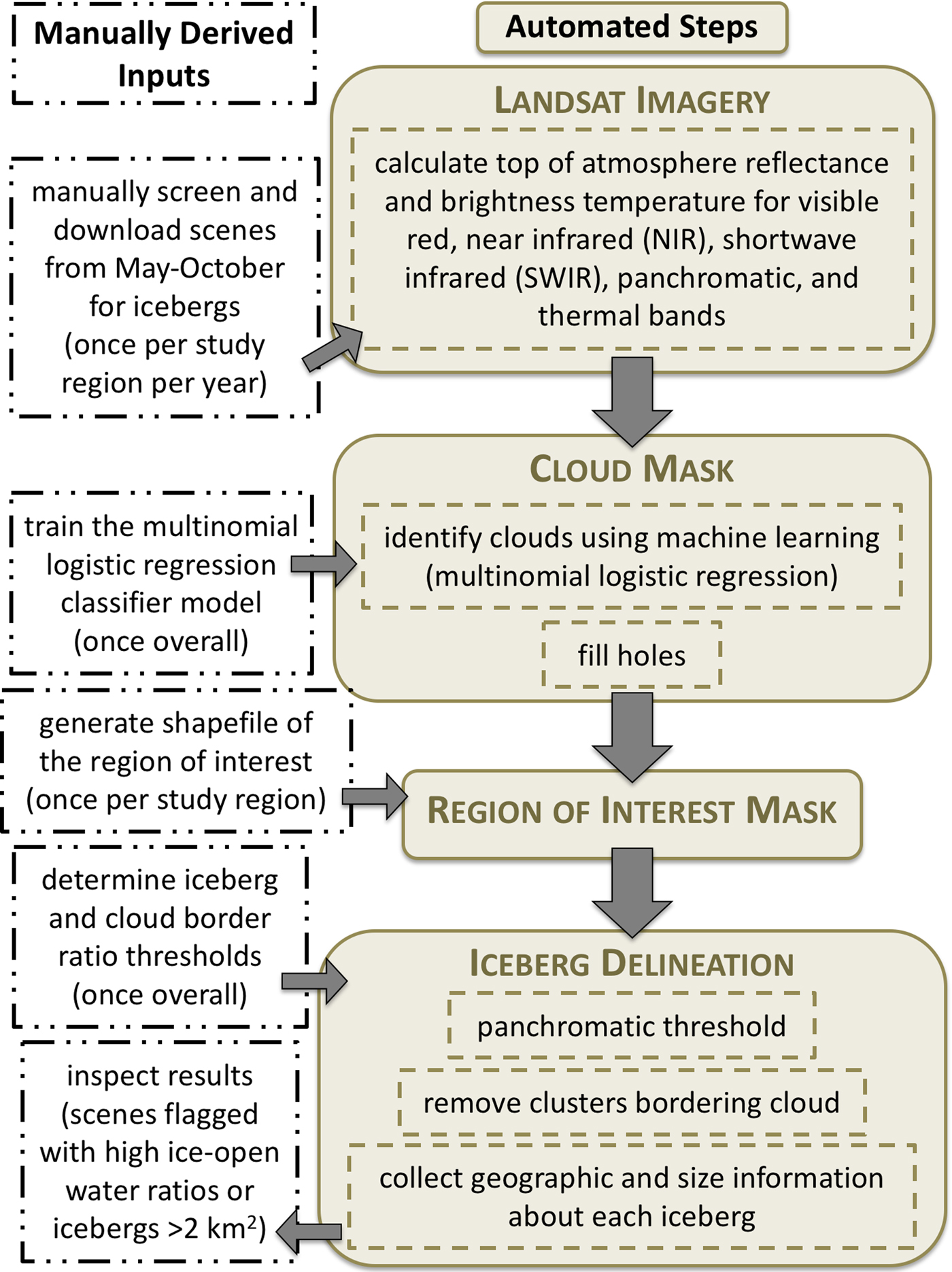
Fig. 2. Schematic illustration of the steps of the final semi-automated iceberg delineation algorithm.
3.2.1. Cloud masking
We tested ratio- and machine learning-based cloud masking techniques, ultimately incorporating a computationally simple, machine learning-based approach into our algorithm (Fig. 2). We inspected and qualitatively evaluated the cloud masks throughout their generation and testing, while quantitative analysis drove development of the final model used in the machine learning-based cloud mask. Example applications of tested methods to an August 2013 Landsat scene (Fig. 3a) are shown in panels b–e of Fig. 3. Here we present only the most common approaches for the sake of brevity since none of the ratio-based methods were used in the final algorithm. These examples capture the essence of the challenge in differentiating icebergs and clouds in optical satellite imagery, illustrating the problems encountered with all tested threshold-based methods, regardless of the choice of threshold or other input parameters.
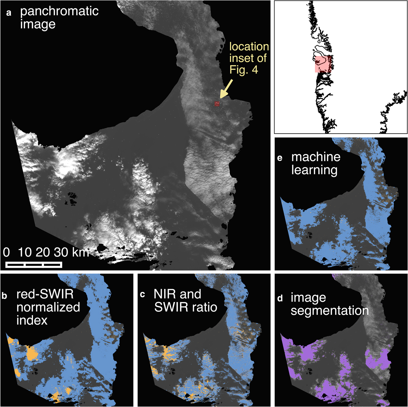
Fig. 3. Comparison of multiple cloud masking and iceberg delineation techniques. (a) Panchromatic (Landsat 8 band 8) scene of Disko Bay from 31 August 2013 showing multiple cloud types. (b–c) Cloud mask (blue) generated using red–SWIR normalized index thresholding and NIR:SWIR ratio combined with SWIR reflectance band thresholding, respectively. Everything above the iceberg delineation threshold after cloud masking is shown in orange. (d) Icebergs and clouds are detected simultaneously using image segmentation (purple). (e) As in (b–c) for the machine learning-based cloud mask.
Ratio-based masks
One approach is to identify clouds simply by applying a threshold to reflectance values in the SWIR part of the spectrum (centered at ~1.6 μm) (e.g. Warren, Reference Warren1982; Dozier, Reference Dozier1989; Riggs and Hall, Reference Riggs and Hall2002). Another approach uses a ratio of the visible red and SWIR bands (wavelengths centered at ~0.66 and 1.6 μm, respectively) (Racoviteanu and others, Reference Racoviteanu, Paul, Raup, Khalsa and Armstrong2009). To further exploit the spectral differences between clouds and snow/ice in these two bands, we computed a normalized index of the two bands (red–SWIR normalized index) (Fig. 3b). We also tested a ratio of the near-infrared (NIR) to SWIR bands (centered at ~0.8 and 1.6 μm, respectively), ultimately generating a ratio-based cloud mask using a combination of the NIR:SWIR ratio and SWIR reflectance (Fig. 3c).
The results produced using the red–SWIR normalized index were similar to those of the individual SWIR reflectance and red:SWIR tests (not shown). The performance of each ratio-based method to distinguish clouds from snow/ice varied widely with cloud type. Very bright, white, fluffy cumulus clouds, which often had similar reflectance values as icebergs, resulted in enough false identifications of clouds and/or icebergs to render the dataset meaningless. The combination of the NIR:SWIR ratio and SWIR reflectance to identify clouds improved the differentiation between clouds and snow/ice over either method alone and over other combinations of the ratio and threshold methods described above (Figs 3b, c) and was thus used as a point of comparison for the performance of our machine learning-based cloud mask. However, the ratio-based method suffered from the same problems as its components, making it ill-suited for unsupervised application to a large number of scenes with diverse cloud types. Further, for all ratio-based methods, the threshold value that best discriminated between clouds and icebergs had to be tailored to each scene (Jedlovec, Reference Jedlovec and Jedlovec2009), requiring extensive operator input and inspection.
Edge detection-based masks
To capitalize on the textural differences between clouds and icebergs rather than relying solely on spectral differences, we tested the ability of edge detection methods to identify features or classify images into segments (i.e. segmentation). These methods could potentially identify icebergs regardless of cloud presence (i.e. only icebergs would be detected), eliminating the need for a cloud masking step. Edge detection uses gradients in reflectance between a pixel and its neighbors to identify transitions in brightness along the edges of distinct objects. Different features are identified in the derived edge maps using feature detection or segmentation methods. Feature detection uses the edge map to isolate and identify objects with certain types of edge characteristics (e.g. fuzzy, gradual edges of clouds or sharp edges of icebergs). Segmentation starts with a series of ‘seeds’, or small groups of pixels, building out from each seed until an edge is reached. The number, size and location of the seeds may be determined automatically, randomly, or manually, with the resulting segmented objects dependent on the number and distribution of seeds. We derived an edge map for a panchromatic Landsat image from August 2013 and tested both feature detection (not shown) and segmentation methods (Fig. 3d). The seeds for segmentation were determined automatically from the original panchromatic image.
The edge detection approaches to identify icebergs or clouds also proved inadequate (Fig. 3d). The feature detection algorithm failed to identify icebergs (or clouds) and was too computationally intensive to run on a laptop. Segmentation suffered from similar problems to the ratio-based approaches; segmentation of iceberg and cloud objects occurred simultaneously, providing no distinctions between clouds and icebergs. This result is unsurprising given that the segmentation map was seeded by applying a conservative reflectance threshold to the panchromatic band, which generally fails to differentiate clouds and ice/snow pixels. Manual seeding may have improved results but would require extensive user input for each scene. Random seeding is also not feasible because it would require dense enough coverage to include a seed in each iceberg and cloud segment (where clouds are present); this would likely lead to over-segmentation of the image. Given the poor performance of the edge detection methods for distinguishing clouds and ice, they were not pursued further.
Machine learning-based masks
To construct the cloud masks ultimately included in our algorithm, we applied a machine learning technique called multinomial logistic regression (Fig. 3e), wherein a classified training set is provided as input and the computer generates a series of functions to relate the image pixel values and their classifications. Then, the model is run on validation datasets and the computer-predicted values are compared to the actual values. To generate training and validation datasets, we manually classified groups of pixels across six scenes with different cloud types as open water, opaque cloud, thin cloud with water underneath, thin cloud with iceberg underneath, or iceberg through clear sky. We extracted the top of atmosphere (TOA) reflectances and brightness temperatures for each classified pixel in the visible, NIR, SWIR and thermal wavelengths. We combined these spectral signatures and associated classifications to create training and validation datasets. Pixels from two scenes, one from each Landsat 7 and 8, were kept separate as a secondary validation dataset, while pixels from the remaining four scenes were randomly split into training and validation sets.
We trained and implemented our multinomial logistic regression model using the Python machine learning scikit-learn library (Pedregosa and others, Reference Pedregosa2011). The generation of models using multiple combinations of bands enabled optimization of the model for accuracy and computation time while minimizing the number of bands involved in masking. Band combinations tested included TOA reflectance/brightness temperature of: (1) red, NIR and SWIR; (2) red, NIR, SWIR and thermal; (3) red, NIR, SWIR, thermal and NIR–SWIR (wavelength centered at ~ 1.63 μm); (4) red, NIR, SWIR, thermal, NIR–SWIR and green wavelengths. We evaluated the model results for each combination of bands for accuracy and found that model performance was similar for all cases (95–97% precision). We eliminated the two options with the largest number of bands (options 3 and 4) to decrease computation requirements and based our final model selection on visual inspection of results. Specifically, we identified commonalities among the misclassified pixels and selected the model where incorrectly classified pixels could most easily be identified and reclassified automatically (e.g. regions of sensor saturation, as described below). The final model selected was option 2.
Two confusion matrices demonstrate the performance of the model by comparing the model's predicted classifications with the manually derived classifications (Table 1). Overall, the machine learning-based cloud mask most consistently and accurately discriminated between bright, white, puffy cumulus clouds and the bright snow/ice surfaces of icebergs. The ratio-based cloud masks only reached comparable accuracy in mapping cloud extent when the cloud border reclassification step was added (see Section 3.2.3). Since this reclassification step relies on a semi-subjective threshold, reliance on its inclusion is not preferred. Manual inspection of the cloud masks also revealed that the ratio-based mask often classified significant amounts of open water as clouds, increasing the number of false negative iceberg detections and decreasing the estimated open water area within the ROI. Given the superior performance of the multinomial logistic regression machine learning-based cloud mask among the methods we tested, we consider it to be the best cloud masking procedure for our analysis.
Table 1. Confusion matrices for the machine learning-based cloud mask for multiple validation sets. The first (Training/Validation) shows the results of the validation dataset from the randomly sampled datasets made up of manually classified pixels from four scenes as outlined in the text. The second (31/08/2013) was generated from a Landsat scene collected 31 August 2013 and only used to validate the model.
u.c. = under cloud
To improve the accuracy of the cloud mask over the central regions of very bright, white cumulus clouds [where cloud type was determined by visual inspection rather than vertical cloud structure or any cloud classification method] where sensor saturation was common, groups of pixels smaller than a ten by ten square structuring element (300 m × 300 m) classified by the model as ice but completely surrounded by pixels classified as clouds were reclassified from ice to cloud and added to the cloud mask. The remainder of the classifications produced by the model were designated non-cloud and small holes in the mask were removed with morphological opening (erosion and then dilation) using a cross-shaped structuring element (Fig. 3e).
The red, NIR, SWIR and thermal bands used to create the cloud mask have a lower spatial resolution (30–100 m pixels) than the panchromatic band (15 m pixels) to which the mask was applied. Thus, we ignored potential mixed pixel effects and assumed that all higher-resolution pixels that fell within the cloud mask were clouds, resulting in a conservatively upsampled (i.e. 15 m resolution) cloud mask. For each scene, we applied the cloud mask to the panchromatic band prior to iceberg identification.
3.2.2. Land/Region of interest mask
To provide a consistent region for analysis that excludes potential land-fast ice and locations with persistent ice mélange, we generated a region of interest (ROI) mask that excludes regions within 100 m of the coastline and all fjords that enter the bay (Fig. 1). Asiaq (personal communication from Asiaq, Greenland Survey, 2014) provided the coastline shapefile used to identify the land boundaries. The ROI mask was applied subsequent to cloud mask application but prior to the iceberg delineation step (Fig. 2).
3.2.3. Iceberg delineation
Following application of the cloud and ROI masks to the TOA reflectance of the panchromatic band, the masked images were used to detect icebergs in the remaining open water regions. Icebergs were identified as pixels with reflectance values in the panchromatic band >0.19. Given the stark contrast in brightness of icebergs from the surrounding water, the iceberg mapping results are fairly insensitive to the threshold value (Figs 4, 5). However, manual inspection of iceberg masks produced using thresholds ranging from 0.17 to 0.21 indicated that a threshold of 0.19 maximized the number of icebergs detected while limiting the number of false positive iceberg detections (i.e. identification of unmasked clouds, sea ice, or rough water as ‘icebergs’). We chose to identify icebergs using thresholding rather than the multinomial logistic regression model ice classification output so that we could optimize the performance of the model for cloud identification.
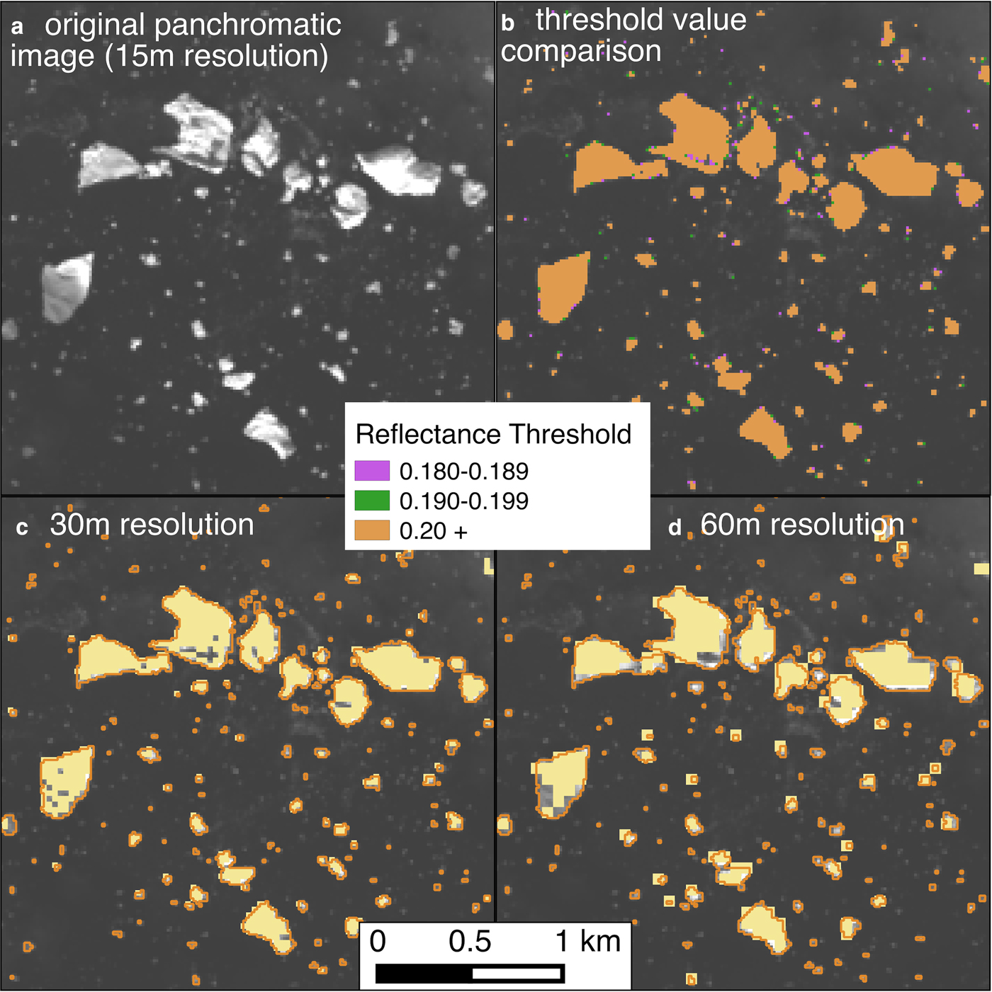
Fig. 4. Influence of threshold choice and image resolution on algorithm performance. Location of panels is shown on Fig. 3. (a) Original panchromatic (Landsat 8 band 8) scene from 31 August 2013. (b) The results of threshold sensitivity tests. Pixels identified as ice by the optimal threshold (0.19) are colored orange and green. (c–d) Automated iceberg masks constructed with the optimal threshold (in yellow), but for 30 m resolution (c) and 60 m resolution (d) images. Orange lines in (c–d) show iceberg outlines derived from the 15 m resolution image.
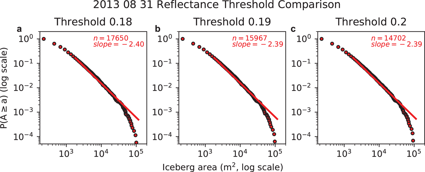
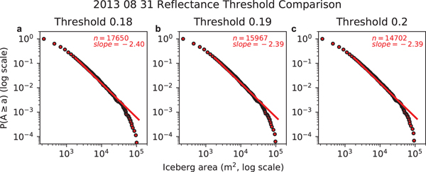
Fig. 5. Iceberg size complimentary cumulative distribution functions for several different reflectance thresholds for the 31 August 2013 scene. Fitted power law curves (in log--log space) show characteristic decay of iceberg areas 1800 m2 and larger, as discussed in the text. n is the total number of icebergs detected, including those smaller than 1800 m2.
After thresholding, adjoining pixels were assumed to be part of the same iceberg and were clustered accordingly. Close visual inspection of the iceberg pixel clusters revealed that in some scenes the edges of clouds missed by the cloud mask were falsely identified as icebergs. Rather than remove the scene from the dataset for abundant false positives (see Section 3.3), pixel clusters that were identified as ice but that bordered cloud along >40% of the cluster's boundary were reclassified as clouds. The remaining clusters were classified as iceberg and outlined automatically by the computer, with each pixel or group of pixels stored as a unique iceberg polygon. To avoid inclusion of portions of icebergs within fjord mouths or along scene boundaries, the algorithm removed any iceberg polygon touching the ROI polygon or a scene edge. The analysis of iceberg parameters presented below uses the resulting shapefiles of iceberg polygons. Total ice area was computed for each shapefile and used in conjunction with the amount of cloud cover and total scene coverage within the ROI to compute an ice–open water ratio.
3.3. Iceberg detection screening of algorithm output
We determined the accuracy and reliability of iceberg detections through semi-automated methods. Scenes with an ice–open water ratio or maximum iceberg area greater than roughly the median plus one median absolute deviation (>0.008 or >2 km2, respectively) were flagged as potential outliers, and we visually inspected scenes with values exceeding these thresholds. For all scenes processed by the algorithm, we overlaid each iceberg shapefile on its corresponding panchromatic scene and visually inspected it at multiple spatial scales. QGIS (QGIS Development Team, 2017) provided the user interface for the inspection, which involved viewing the entire scene as well as taking a closer look at common problem areas such as along the borders of clouds or clusters of closely spaced small icebergs.
We excluded 11 of the 65 scenes run on the basis of this quantitative screening and manual inspection, leaving 54 scenes for the 6 years included in our study with 7–12 data points per year (mean: 9 acquisition dates per year). Reasons for exclusion included: (1) non-detection of large numbers of icebergs greater than one or two pixels in size; (2) large numbers of false positive detections of water, clouds and/or sea ice as icebergs. Wispy, semi-transparent cirrus clouds covered substantial portions of all but two of the scenes that were excluded on the basis of false detections; the false positive detections in these two scenes resulted from sea ice or water. The presence of cirrus clouds was limited or nonexistent in all other cloudy scenes. Six of the eleven scenes excluded during this step had maximum iceberg size or ice–open water ratio values exceeding the quantitative thresholds. Thus, this inspection of results suggests that although there is no way to automatically screen for rare scenes with a large number of missed icebergs, the majority of results dominated by false positive signals can be detected and eliminated automatically through the use of ice coverage and iceberg size cutoffs.
4. RESULTS
4.1. Total iceberg area
We evaluated algorithm performance by running the algorithm on several Landsat Collection scenes (20 August 2013, 7 August 2014 and 26 August 2015) covering Kangerlussuup Sermia Fjord, scenes for which Sulak and others (Reference Sulak, Sutherland, Enderlin, Stearns and Hamilton2017) previously established total iceberg areas. To match the methodology of Sulak and others (Reference Sulak, Sutherland, Enderlin, Stearns and Hamilton2017) as closely as possible, we ran the algorithm as designed as well as with a higher reflectance threshold (0.28), without the land buffer and without the step removing partial icebergs captured along the ROI and scene borders. The cloud mask was run in each case, even though Sulak and others (Reference Sulak, Sutherland, Enderlin, Stearns and Hamilton2017) manually selected the images as cloud-free. This resulted in very limited (<0.08%) cloud cover over the area of interest, illustrating that our cloud mask successfully avoids false positives.
At Kangerlussuup Sermia Fjord, iceberg areas derived using our algorithm are consistent with previous values (Table 2) (Sulak and others, Reference Sulak, Sutherland, Enderlin, Stearns and Hamilton2017). Percent differences for total iceberg area vary by <10% and are non-systematic. Our inability to precisely reproduce the total iceberg areas exactly can at least partially be explained by the potential differences in the ROI extent within the fjord, particularly near the glacier terminus but also at the fjord mouth. As expected, application of a buffer to land areas and removal of polygons intersecting our ROI polygon causes the percent error to become increasingly positive, because this step reduces the total ice area. Although the impact of these components of our algorithm on total ice area can reach up to 22.1% of the iceberg area calculated by Sulak and others (Reference Sulak, Sutherland, Enderlin, Stearns and Hamilton2017), the absolute difference in ice area is quite small because the ice makes up such a small portion of the total area (the ice–open water ratio changes from 0.0045 to 0.0035).
Table 2. Total iceberg areas for Kangerlussuup Sermia Fjord, shown as percent variation from Sulak and others (Reference Sulak, Sutherland, Enderlin, Stearns and Hamilton2017) given choice of reflectance threshold, application of land buffer, and removal of partial icebergs included along the borders of a polygon defining the area of interest
* Sulak and others (Reference Sulak, Sutherland, Enderlin, Stearns and Hamilton2017)
Interestingly, we found that application of the Disko Bay threshold to identify icebergs in Kangerlussuup Sermia Fjord resulted in an apparent overestimation of iceberg area relative to Sulak and others (Reference Sulak, Sutherland, Enderlin, Stearns and Hamilton2017). An increase in the threshold from 0.19 to 0.28 considerably decreased this overestimation of iceberg area in all three scenes, indicating that site-specific thresholds are necessary to calculate ice area. Further analysis of the data shows that although the lower threshold values may lead to a systematic bias in ice area estimates, the number of detected icebergs remains fairly consistent between the two thresholds. We attribute the disparate threshold sensitivity of the iceberg area and number estimates to the mixed-pixel effect: pixels around iceberg margins that are primarily water but contain a small fraction of ice will be detected at lower thresholds, inflating the iceberg area estimates while preserving the iceberg number estimates. Thus, use of regional (i.e. not site-specific) thresholds in future analyses may bias iceberg area estimates but are unlikely to influence iceberg size distributions.
4.2. Iceberg size distributions
Iceberg size distributions around Antarctica and Greenland have previously been characterized using both power law and lognormal distributions (e.g. Tournadre and others, Reference Tournadre, Girard-Ardhuin and Legrésy2012; Enderlin and others, Reference Enderlin, Hamilton, Straneo and Sutherland2016; Kirkham and others, Reference Kirkham2017; Sulak and others, Reference Sulak, Sutherland, Enderlin, Stearns and Hamilton2017). We tested power law, lognormal, exponential and Weibull distributions using the Python powerlaw (Alstott and others, Reference Alstott, Bullmore and Plenz2014) library on two scenes' size distributions and found that a power law distribution of the form f(x) = x −α, where α is the fit parameter or slope of the probability distribution in log--log space (Fig. 5), weakly but consistently provided the best fit (see the Supplementary Material for an explanation and evaluation of fit parameters).
Since our primary interest here is a consistent way to quantitatively describe the data and its variations through time, rather than necessarily capturing the exact shape of the distribution, we fit power law size distributions to each date's iceberg dataset using an x min value of 1800 m2 (eight pixels). Although the algorithm can detect smaller icebergs (down to 1–2 pixels), we chose this x min value because it generally has a minimal fit uncertainty when compared with the fit uncertainties of other x min values. Using a lower x min value influences the fit parameter values (Clauset and others, Reference Clauset, Shalizi and Newman2009) due to large fluctuations in the smaller size fractions of icebergs, resulting in less robust fits and suggesting that the smallest icebergs do not follow the same size distribution. Conversely, using the much higher x min values suggested by the software results in data loss. A detailed discussion of the challenges and limitations associated with rigorous fitting of heavy-tailed size distributions is provided in the Supplementary Material.
4.3. Error analysis
4.3.1. Iceberg size distribution sensitivity to choice of reflectance threshold.
Satellite image-derived iceberg size distributions are fairly insensitive to the choice of the reflectance threshold used to identify icebergs in the cloud-masked scenes, provided the threshold value is tailored to the study site (Figs 4, 5). Specifically, modification of the reflectance threshold by ~5% (~10%) to 0.18 and 0.20 (0.17 and 0.21) resulted in changes in the slope of the power law fits of <0.4% (<0.9%). Even large changes in threshold values (e.g. ~50%) resulted in comparatively small (<9%) changes in the fitted power law slope, although the uncertainties in ice coverage and number of icebergs (>50–100%) were close to the proportional changes in threshold. Manual inspection of the results from these large threshold variations shows the lower threshold resulted in an increase in the number of false negatives and the higher threshold resulted in an increase in the number of false positives from other noise in the image. Regardless, the small changes in slope even with large changes in the threshold value suggest that the fitted power law slope remains a robust metric to describe the size distribution.
4.3.2. Spatial sampling: generation of scene mosaics and upsampling of lower resolution bands.
Since Landsat scenes utilize the UTM projection, the generation of mosaics often requires reprojection of one scene so that the same UTM zone is used by both scenes in the mosaic. During mosaicking, pixel values in overlapping portions of the scenes are averaged. Due to coregistration errors, which can skew the location of icebergs between scenes, pixel averaging has the potential to lead to both false positive and false negative iceberg identifications; iceberg pixel values may drop below the threshold used for iceberg detection, causing icebergs to be missed, or small icebergs may be double-counted. In line with previous studies, careful qualitative inspection of the overlapping region of several mosaics suggests that the geolocation errors are on the order of the pixel resolution (Storey and others, Reference Storey, Choate and Lee2014) and are sufficient for image mosaicking without compromising the detectability of icebergs or resulting in double counting of small icebergs. The impact of upsampling to match the highest spatial resolution bands is limited to the application of our cloud mask to the panchromatic image. Our iceberg size distributions are similar within a given time period regardless of the amount of cloud cover in a particular scene, suggesting that the upsampling of our cloud mask to match the spatial resolution of the panchromatic band does not affect our results.
5. DISCUSSION
5.1. Disko Bay icebergs
Beginning in 1997, Sermeq Kujalleq underwent a period of rapid retreat, thinning and acceleration that included the loss of a persistent floating ice tongue in the early 2000s (e.g. Joughin and others, Reference Joughin, Abdalati and Fahnestock2004; Luckman and Murray, Reference Luckman and Murray2005; Holland and others, Reference Holland, Thomas, de Young, Ribergaard and Lyberth2008; Bondzio and others, Reference Bondzio2017). As the terminus of Sermeq Kujalleq transitioned to a terminus grounded in deeper water, the dominant calving style shifted from infrequent calving of tabular icebergs towards more frequent calving and overturning of full thickness icebergs and smaller partial-thickness icebergs (e.g. Amundson and others, Reference Amundson2008; Joughin and others, Reference Joughin2008; Bassis and Jacobs, Reference Bassis and Jacobs2013; Cassotto and others, Reference Cassotto, Fahnestock, Amundson, Truffer and Joughin2015). This change in calving style, and consequently calving energy (Bassis and Jacobs, Reference Bassis and Jacobs2013), produced icebergs with different geometries. Since iceberg decay is strongly controlled by iceberg geometry, we explored whether the change in Sermeq Kujalleq's calving could be inferred from a shift in iceberg size distributions.
We applied the semi-automated algorithm, using the machine learning-based cloud mask, to the Landsat archive for Disko Bay from 2000–02 and 2013–15 (Fig. 6). We chose these year ranges to span the time period of greatest change in calving behavior of Sermeq Kujalleq (Amundson and others, Reference Amundson2008; Joughin and others, Reference Joughin2008) as well as avoid missing icebergs in whole or in part due to the stripping caused by the SLC failure on Landsat 7. Although methods exist to ‘fill in’ the missing data, these methods rely on landscape continuity through space or over time. The transient nature of icebergs means there is no reliable way to fill in the image gaps, thereby limiting the accuracy of an iceberg size dataset derived from this imagery.
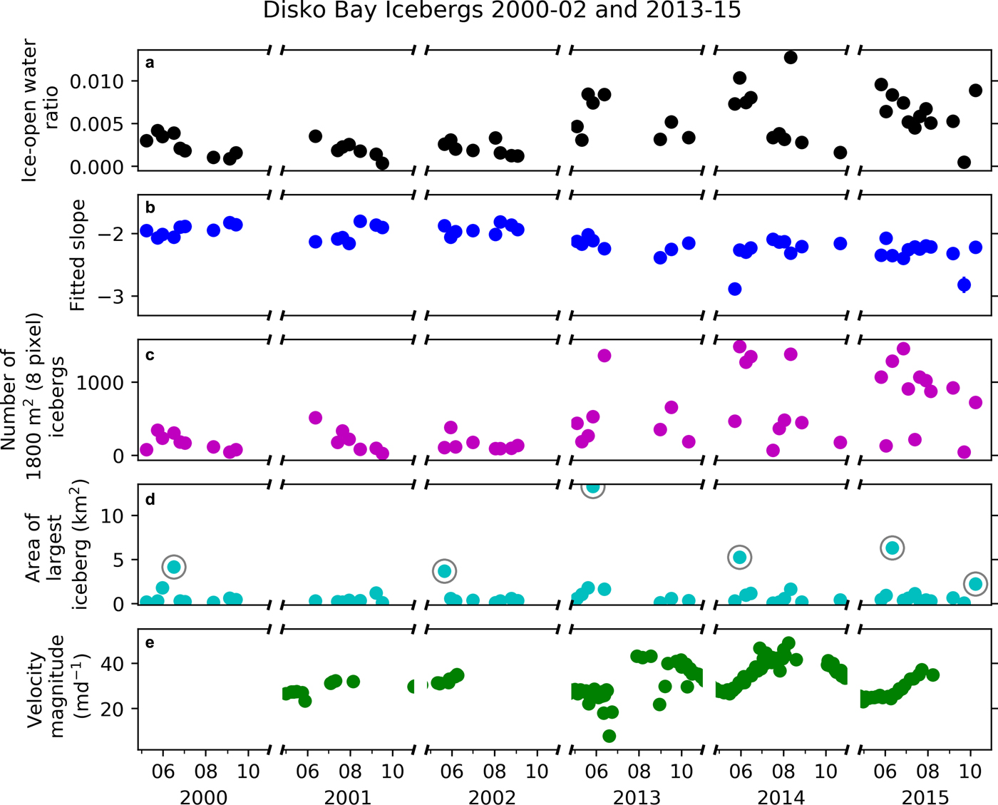
Fig. 6. Iceberg data extracted from Landsat scenes spanning 2000–02 and 2013–15. (a) Ice–open water ratio. (b) The slope of the power law curve fit to the iceberg size distribution for each scene. Error bars showing the goodness of fit of the slope to the distribution are obscured by the symbol in almost all cases. (c) Number of eight pixel (1800 m2) icebergs. (d) Plan view area of the largest iceberg. Circled points are sea ice > 2 km2 detected in scenes not excluded from our results as discussed in the text. (e) Surface velocity magnitude 1 km upstream of the terminus.
5.2. Ice cover and iceberg size distributions
Ice coverage is a function of the total ice-covered and open water areas relative to the observed area for that scene, which we present as an ice–open water ratio (Fig. 6a) to account for differences in scene extent and cloud cover. The ice cover in Disko Bay has evolved in conjunction with the changes at the terminus of Sermeq Kujalleq (Fig. 6a). During the later time period (2013–15), the median and range of ice–open water ratios is notably larger relative to the turn of the century (2000–02) (median±MAD of 0.0019 ± 0.0007 and 0.0056 ± 0.0022 for the two time periods, respectively).
The fitted power law slopes representing our iceberg size distributions fall within the range −1.80 to −2.89, with a median of −2.12 (Fig. 6b), in agreement with previously published values for iceberg size distributions in Greenland's fjords (−1.9 to −2.3 in Enderlin and others (Reference Enderlin, Hamilton, Straneo and Sutherland2016) and −1.62 to −2 in Sulak and others (Reference Sulak, Sutherland, Enderlin, Stearns and Hamilton2017)). The fitted power law slopes have a mean goodness of fit error of 0.024 and an uncertainty of <0.4%, calculated as the change in slope value resulting from a ~5% change in the ice detection threshold value. Interestingly, the size distributions of icebergs in the bay suggest a small but significant decrease in slope values between the two time periods. For 2000–02, the median slope was −1.96 (± 0.03) while for 2013–15 the median slope was −2.26 (± 0.02). Although submarine melting of icebergs will also affect iceberg size distributions (Kirkham and others, Reference Kirkham2017), we hypothesize that temporal changes in submarine melting had little influence on the observed shift in iceberg size distributions for two reasons. First, subsurface ocean observations in Disko Bay suggest that the waters in the bay warmed in the late 1990s and have remained relatively warm since then (Holland and others, Reference Holland, Thomas, de Young, Ribergaard and Lyberth2008; Gladish and others, Reference Gladish, Holland, Rosing-Asvid, Behrens and Boje2015). Second, oceanic warming will preferentially decrease the abundance of small icebergs due to their high surface area to volume ratios, with warmer near-surface water temperatures driving increased melt. This will effectively remove icebergs in the smallest size fractions and will likely manifest in iceberg size distributions as a shift from fitted power law to lognormal size distributions (Kirkham and others, Reference Kirkham2017), potentially explaining the increases in power law fit parameter uncertainty with the use of x min values <1800 m2. If we consider that the total volume of melt is a function of both the melt rate and time period, then we can look at changes in iceberg size distributions with distance from the source as an analog for changes in the magnitude of melting. As such, the shift towards a lognormal iceberg size distribution observed by Kirkham and others (Reference Kirkham2017) suggests that any melt-driven changes in the size distribution would be counter to what we observe. Alternatively, a decreased presence of sea ice would tend to drive an increase in wave erosion, leading to enhanced mechanical iceberg decay and providing an alternative explanation for the change in fitted power law slope between the two time periods. However, changes in sea ice cover likely occurred prior to the turn of the 21st century when waters in Disko Bay warmed, prior to the start of our investigation.
The observed changes in ice cover and slope of the size distribution are likely driven by the concurrent increase in the number and frequency of times that a large number of 1800 m2 (eight pixel) icebergs are present in the bay (Fig. 6c). During 2000–02, none of the scenes analyzed have >1000 icebergs in the smallest size bin (1800 m2) and only one scene has >500 small icebergs, whereas during 2013–15 at least an eighth of the scenes have >1000 small icebergs and over a third of scenes have >500 small icebergs. The increased presence of small icebergs between the 2000–02 and 2013–15 observation periods drives the steepening of the fitted power law slope (Fig. 6b) and matches anecdotal evidence from boat captains operating in Disko Bay, who lamented the difficulty of navigating and setting long fishing lines in the mid 2010s due to the large number of small icebergs present in the bay. We interpret this change in the abundance of small icebergs in the bay as a consequence of the change in the dominant calving style of Sermeq Kujalleq. As the glacier's terminus geometry evolved from persistently-floating and seasonally-grounded (Joughin and others, Reference Joughin2008), the associated increase in calving energy resulted in an increase in iceberg fragmentation and thus an increase in the number of smaller icebergs in Disko Bay.
The maximum size of icebergs detected in Disko Bay remained relatively constant during this time period (Fig. 6d). Some icebergs >2 km2 (approximately an order of magnitude magnitude larger than the maximum size of icebergs able to pass over the sill in Ilulissat Isfjord) were not excluded from our results because manual inspection (see Section 3.3) revealed that they are localized areas of potentially unnavigable sea ice that have little influence on the derived ice–open water ratio.
5.3. Comparison of icebergs and parent glacier dynamics
Recent numerical modeling of calving dynamics suggests that changes in calving style result from changes in glacier terminus relative buoyancy, defined as the water depth at the terminus relative to the water depth required for ice flotation (Benn and others, Reference Benn2017). We calculated the relative buoyancy of Sermeq Kujalleq's terminus to determine whether changes in relative buoyancy, and thus calving dynamics, could have driven the observed changes in iceberg sizes and ice cover in Disko Bay. We extracted ice surface elevation from pre-IceBridge (late May 2001/02 and 2013–15; no data were available for 2000) (Thomas and Studinger, Reference Thomas and Studinger2010) and WorldView image-derived digital elevation models (DEMs; late June through late September 2013–15) (DEMs were created by the Polar Geospatial Center from DigitalGlobe, Inc. imagery) and water depth (bed elevation) from BedMachine v3 (Morlighem and others, Reference Morlighem2017) at a point located 1 km upstream of the terminus. Ice thickness was estimated assuming buoyancy (density of sea water and ice were taken as 1027.3 kg m−3 and 900 kg m−3, respectively). If the thickness of the presumed floating ice exceeded the bed depth, then the ice was considered grounded and the ice thickness was instead calculated as the difference between the ice surface elevation and the bed depth. The water depth required for ice flotation was calculated following Eqn (4) in Benn and others (Reference Benn2017) and used as input for relative buoyancy estimates. Prior to 2002, minimum May relative buoyancy values were ~2, well beyond the ‘super-buoyant’ threshold of 1.1 suggested by Benn and others (Reference Benn2017). From 2013–15, relative buoyancy values in April were ~1.1, while those from the summer were ~0.84, demonstrating that the terminus had shifted from a super-buoyant floating ice tongue to a barely floating and seasonally well grounded terminus (Benn and others, Reference Benn2017).
The change in terminus geometry since the early 2000s is also reflected in the record of near-terminus velocity for Sermeq Kujalleq (Fig. 6e). We extracted Landsat-derived surface velocities for 2001, 2002 and 2013–15 from the Technische Universität Dresden Velocity Fields of Greenland Outlet Glaciers data product (Rosenau and others, Reference Rosenau, Scheinert and Dietrich2015) at the same locations as the ice thickness data above. The time series clearly illustrates an increased seasonal signal in Sermeq Kujalleq's velocity (Joughin and others, Reference Joughin, Smith, Shean and Floricioiu2014) and is indicative of the glacier's increased responsiveness to changes in backstress at the terminus as a result of the loss of its floating ice tongue and corresponding change in calving style (Joughin and others, Reference Joughin2012).
6. CONCLUSIONS
We have presented a semi-automated approach to delineate icebergs in optical (Landsat) satellite images. To test the performance of the approach and demonstrate its utility, we provide an example application to Landsat images for Disko Bay, West Greenland. The images span the years 2000–02 and 2013–15, capturing important changes in the calving style of Sermeq Kujalleq.
A challenge in automated detection of icebergs in optical imagery is differentiation of clouds and snow/ice, due to their similar spectral properties, and cloud masking often requires a large number of steps and/or advanced computing capabilities. To eliminate clouds from our scenes, we developed a computationally efficient cloud masking scheme using machine learning to identify clouds. A comparison of multiple cloud masks for the same scenes suggests that the machine learning-based cloud mask performs better than the commonly used ratio-based approaches to delineate clouds. Thus, we recommend that studies leverage similar machine learning-based cloud masking approaches to utilize Landsat scenes with partial cloud cover over glaciers and sea ice.
We applied our semi-automated algorithm to a series of Landsat images from 2000–02 and 2013–15. After clouds and land were masked out of each scene using the machine learning-based cloud and ROI masks, respectively, the remaining portions of the TOA reflectance of the panchromatic band were thresholded to detect icebergs. Based on a comparison with previously published total ice area values for Kangerlussuup Sermia Fjord (Sulak and others, Reference Sulak, Sutherland, Enderlin, Stearns and Hamilton2017), we found that while the total ice area in that region was readily influenced by the choice of threshold value, in Disko Bay, the slope of the power law curve describing the iceberg size distributions was insensitive to the choice of threshold value.
Our results show that the size distributions of icebergs in Disko Bay underwent an important transition from the early 2000s (2000–02) to the mid 2010s (2013–15), concurrent with a transition in Sermeq Kujalleq's dominant calving style. Between 2000–02 and 2013–15, we observed a pronounced increase in the total ice cover, decrease in the power law slope describing the distribution of iceberg sizes and increase in the number of small icebergs in Disko Bay. The temporal change in the number of small icebergs present supports anecdotal evidence from local marine navigators, who were adversely impacted by the shift. These observed changes were coincident with a change in the calving style of Sermeq Kujalleq from low energy calving of tabular icebergs to high energy calving of full thickness icebergs. The change in calving style was driven by a change in terminus geometry from a persistently-floating ice tongue to a seasonally well-grounded terminus. Both decadal-scale change in glacier terminus buoyancy and increased seasonality in velocity due to terminus retreat and grounding supported the change in calving style. Based on these concurrent changes, we conclude that changes in calving style have an appreciable influence on iceberg size distributions. Expansion of this case study to gain a better understanding of how glacier dynamics and iceberg decay processes impact iceberg size distributions across multiple spatial and temporal scales is critical for improving our understanding of how iceberg presence changes through time and its potential future impacts on navigation and distributed freshwater flux in coastal systems.
SUPPLEMENTARY MATERIAL
The supplementary material for this article can be found at https://doi.org/10.1017/jog.2019.23
CONTRIBUTION STATEMENT
JS and GH designed the project and JS carried out the algorithm development and application with feedback from GH and EE. JS prepared the manuscript with contributions from EE.
ACKNOWLEDGMENTS
This work was supported by NASA Headquarters under the NASA Earth and Space Science Fellowship Program (grant NNX15AP08H, awarded to JS), NASA via the Maine Space Grant Consortium (award to JS), and the US National Science Foundation Adaptation to Abrupt Climate Change IGERT Program (grant DGE-1144423). We thank Jakob Abermann and Eva Mätzler and others at Asiaq, Greenland Survey, for assisting with project development and insightful discussions on iceberg detection and icebergs along the west coast of Greenland. We also thank the many marine operators and other residents of Nuuk and Ilulissat who provided information on iceberg hazards in Disko Bay and helped shape the goals of this project. Feedback from Helen Fricker and two anonymous reviewers significantly improved the manuscript.


 Open access