


1. Introduction
The coast near Boulogne-sur-Mer in NW France offers a well-exposed succession of Upper Jurassic sandstone units alternating with organic-rich mudstones. This study focuses on one of these organic-rich mudstone units, the Argiles de Châtillon Formation (ACF). The ACF is a proximal analogue for the Kimmeridge Clay Formation (KCF) that crops out in southern England and is an important source rock in the North Sea Basin (Herbin et al. Reference Herbin, Fernandez-Martinez, Geyssant, Albani, Deconinck, Proust, Colbeaux and Vidier1995; Proust et al. Reference Proust, Deconinck, Geyssant, Herbin and Vidier1995; Tribovillard et al. Reference Tribovillard, Ramdani, Trentesaux and Harris2005; Cornford, Reference Cornford, Turner and Cronin2018). The KCF consists predominantly of laminated mudstones, intercalated with limestones and dolostones, indicating a relatively distal marine depositional environment. The less complete and more proximal ACF is characterized by more bioturbated mudstones, thin sandstones and storm-induced bioclastic limestones. Based on ammonite biostratigraphy, the age of the ACF is latest Kimmeridgian to earliest Tithonian (Geyssant et al. Reference Geyssant, Vidier, Herbin, Proust and Deconinck1993; Herbin et al. Reference Herbin, Fernandez-Martinez, Geyssant, Albani, Deconinck, Proust, Colbeaux and Vidier1995), which corresponds to the middle part of the KCF.
The ACF is stratigraphically sandwiched between two prominent sandstone units, the Grès de Châtillon Formation below and the Grès de la Crèche Formation above (Fig. 1). Halfway through the 20 m thick succession of the ACF, an erosive unconformity, interpreted as a sequence boundary (Wignall & Newton, Reference Wignall and Newton2001), subdivides the formation into a lower and an upper member (Fig. 1). Two distinct organic-rich intervals (ORIs) occur in the ACF, one near the base of the lower member and one in the lower part of the upper member. These display total organic carbon (TOC) contents of a maximum of 8 %, but TOC contents are laterally variable (Herbin et al. Reference Herbin, Fernandez-Martinez, Geyssant, Albani, Deconinck, Proust, Colbeaux and Vidier1995; Tribovillard et al. Reference Tribovillard, Bialkowski, Tyson, Lallier-Verges and Deconinck2001). Sequence stratigraphic studies allow the correlation of the two ORIs to periods of rising and high sea level (Proust et al. Reference Proust, Mahieux and Tessier2001; Wignall & Newton, Reference Wignall and Newton2001). However, according to others, sea level is not the sole factor controlling organic matter (OM) enrichment. Changes in global climate, driving changes in primary productivity, may have played an equally important role (Herbin et al. Reference Herbin, Fernandez-Martinez, Geyssant, Albani, Deconinck, Proust, Colbeaux and Vidier1995). Moreover, it was recently proposed that the two ORIs in the ACF are the result of different driving forces, with the lower interval deposited under calm and restricted conditions, and the upper interval deposited under oxic and more energetic conditions (Tribovillard et al. Reference Tribovillard, Koched, Baudin, Adatte, Delattre, Abraham and Ferry2019). The apparent contradiction of OM enrichment under oxic conditions is explained by assuming a system of storm-induced OM concentration. According to these authors, sulfurization occurred in more proximal environments and storms remobilized the OM to the oxygenated, shallow-marine setting. The chemically recalcitrant structure of the sulfurized OM made it resistant against oxidation after deposition.
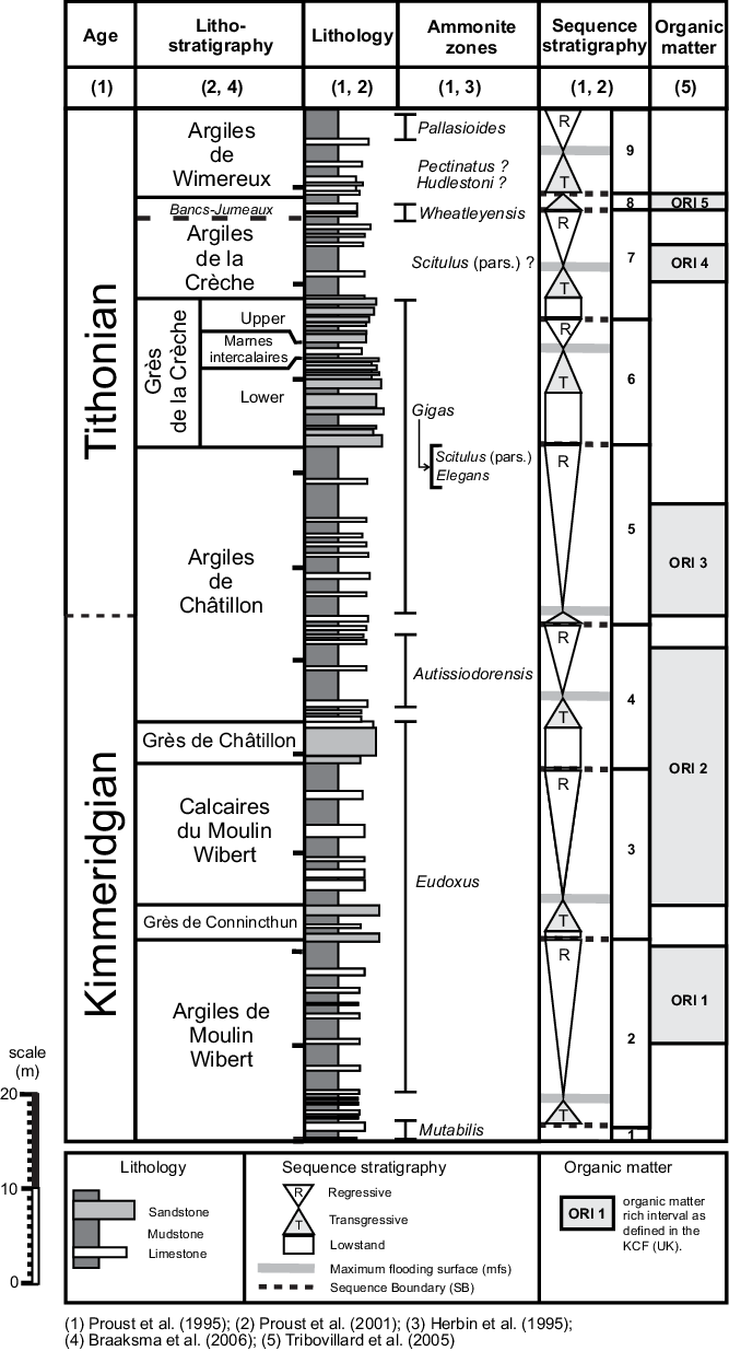
Fig. 1. Stratigraphic framework of the Upper Jurassic succession from the Boulonnais area, displaying the lithostratigraphy, chronostratigraphy sequence stratigraphy, and organic matter rich intervals.
The ACF spans the transition from the Kimmeridgian to the Tithonian (Gallois et al. Reference Gallois, Vadet and Etches2019), a period that records a climate change in NW Europe, evolving from warm and humid conditions in late Kimmeridgian time (Eudoxus and Autissiodorensis ammonite zones) to more arid conditions in early Tithonian time (Elegans ammonite Zone; Abbink et al. Reference Abbink, Targarona, Brinkhuis and Visscher2001; Deconinck & Baudin, Reference Deconinck and Baudin2008; Hesselbo et al. Reference Hesselbo, Deconinck, Huggett and Morgans-Bell2009). Smaller-scale Milankovitch cyclicity-controlled climate variations have been recorded in the ACF as well as in the KCF, with alternations on a decimetre–metre scale (e.g. Waterhouse, Reference Waterhouse, House and Gale1995, Reference Waterhouse1999; Weedon et al. Reference Weedon, Jenkyns, Coe and Hesselbo1999; Huang et al. Reference Huang, Hesselbo and Hinnov2010).
The present study aims to understand the relationship between variations in Late Jurassic climate, regional carbon isotope trends and OM distribution of the Upper Jurassic ACF. Because of its relatively proximal marine setting, the ACF is adequately suited for palynological analysis, as it provides a balanced mix between land-derived and marine palynomorphs. The land-derived palynomorphs are expected to reflect trends in vegetation and, by inference, climate. We aim to investigate if and how climate change controlled the OM distribution in the ACF. In addition, the ACF and the base of the overlying Grès de la Crèche Fm have been sampled in high resolution for stable isotope analysis (δ13Corg) in order to correlate the Boulonnais outcrops to the regional record from the KCF (Morgans-Bell et al. Reference Morgans-Bell, Coe, Hesselbo, Jenkyns, Weedon, Marshall, Tyson and Williams2001). An accurate correlation between the ACF and KCF will allow comparison between OM accumulation processes in the proximal and distal domains and establish an OM accumulation model for the latest Kimmeridgian – earliest Tithonian period that is applicable on a basin-wide scale.
2. Geological setting
During Kimmeridgian and Tithonian times, Western Europe was composed of an archipelago of low-lying massifs set in a broad and relatively shallow epicontinental sea, the Laurasian Seaway (Ziegler, Reference Ziegler1990; Fig. 2). The Laurasian Seaway connected the Panboreal Superrealm in the north to the Tethys Ocean to the south. This area comprises a series of interconnected basins, such as the Paris, Wealden, Cleveland and Wessex basins, that evolved as a result of the break-up of Pangaea that started in the Triassic Period (Underhill & Stoneley, Reference Underhill, Stoneley and Underhill1998; Mansy et al. Reference Mansy, Manby, Averbuch, Everaerts, Bergerat, van Vliet-Lanoë, Lamarche and Vandycke2003; Zanella & Coward, Reference Zanella, Coward, Evans, Graham, Armour and Bathurst2003). Estimations of the water depth in these basins varied between several tens of metres (e.g. Hallam, Reference Hallam1975) and hundreds of metres (e.g. Herbin et al. Reference Herbin, Muller, Geyssant, Melieres and Penn1991).

Fig. 2. Palaeogeographic map of NW Europe for the Late Jurassic period showing the locations of the Boulonnais area in relation to other basins and emergent land masses. B – Boulonnais; WB – Wessex Basin; PB – Paris Basin; CB – Cleveland Basin; BFB – Broad Fourteens Basin; CG – Central Graben; VG – Viking Graben; LBM – London–Brabant Massif; AM – Armorican Massif. Modified after Coward et al. (Reference Coward, Dewey, Hempton, Holroyd, Evans, Graham, Armour and Bathurst2003).
The sediments of the ACF were deposited at the easternmost edge of the Wessex Basin, bounded in the north by the London–Brabant Massif (Fig. 2). The Wessex Basin was periodically anoxic, alternating with shorter or longer oxygenation events (Oschmann, Reference Oschmann1988; van Kaam-Peters et al. Reference van Kaam-Peters, Schouten, de Leeuw and Sinninghe Damsté1997; Waterhouse, Reference Waterhouse1999). As part of a clastic-dominated ramp environment, the Boulonnais area accumulated sand-dominated deposits alternating with silt and clay-dominated deposits. Sedimentation was controlled by relative sea level (Proust et al. Reference Proust, Deconinck, Geyssant, Herbin and Vidier1995; Braaksma et al. Reference Braaksma, Drijkoningen, Filippidou, Kenter and Proust2006) and affected by synsedimentary faulting (Hatem et al. Reference Hatem, Tribovillard, Averbuch, Vidier, Sansjofre, Birgel and Guillot2014). Multiple studies of the Boulonnais sections have provided a depositional and sequence stratigraphical framework that is useful to correlate and compare the different outcrops and to explain variations in OM content (Herbin et al. Reference Herbin, Fernandez-Martinez, Geyssant, Albani, Deconinck, Proust, Colbeaux and Vidier1995; Proust et al. Reference Proust, Deconinck, Geyssant, Herbin and Vidier1995; Deconinck et al. Reference Deconinck, Geyssant, Proust and Vidier1996; Wignall et al. Reference Wignall, Sutcliffe, Clemson and Young1996; Tribovillard et al. Reference Tribovillard, Bialkowski, Tyson, Lallier-Verges and Deconinck2001; Wignall & Newton, Reference Wignall and Newton2001; Braaksma et al. Reference Braaksma, Drijkoningen, Filippidou, Kenter and Proust2006; Deconinck & Baudin, Reference Deconinck and Baudin2008; Hatem et al. Reference Hatem, Tribovillard, Averbuch, Bout-Roumazeilles, Trentesaux, Deconinck, Baudin and Adatte2017).
The most complete and best accessible outcrops of the ACF and the underlying Grès de Châtillon Fm occur between the village of Audresselles and Cap Gris Nez (Fig. 3). The 5 m thick Grès de Châtillon Fm consists of thin carbonate cemented sandstones with clay partings, common cross-bedding, wave ripples and trace fossils such as Rhizocorallium, Ophiomorpha and Thalassinoides (Wignall et al. Reference Wignall, Sutcliffe, Clemson and Young1996; Schlirf, Reference Schlirf2003). The sandstones were deposited in a tidally influenced, shallow-marine setting and are shallowing-upwards (Proust et al. Reference Proust, Deconinck, Geyssant, Herbin and Vidier1995; Braaksma et al. Reference Braaksma, Drijkoningen, Filippidou, Kenter and Proust2006; Angus et al. Reference Angus, Hampson, Palci and Fraser2020). A conspicuous 1 m thick uncemented and heterogeneous sandstone with bright orange colours marks the top of the formation and is laterally continuous over several kilometres (Fig. 5b). Crocodile teeth (pers. obs.), charcoal fragments, bioclastic gravel strings (Angus et al. Reference Angus, Hampson, Palci and Fraser2020) and features indicating synsedimentary faulting (Hatem et al. Reference Hatem, Tribovillard, Averbuch, Vidier, Sansjofre, Birgel and Guillot2014, Reference Hatem, Tribovillard, Averbuch, Sansjofre, Adatte and Guillot2016) occur in this layer.

Fig. 3. Overview of the Boulonnais area and location of the three studied sections, the Cran aux Œufs, Cran du Noirda and Cap de la Crèche sections. For the palaeogeographic position of the Boulonnais in NW Europe/Wessex Basin, see Figure 2.

Fig. 4. Lithological log of the Cran aux Œufs section. The subsections bearing sample codes OEB and OEF are correlated via a marker bed on top of a small unexposed interval, marked with a cross. The position of the stage, ammonite zone and member boundaries are based on the δ13Corg correlations. Outcrop pictures are displayed in Figure 5.

Fig. 5. Outcrop pictures from the Cran aux Œufs section. (a) Subsection OEF, representing the upper part of the Cran aux Œufs section that covers the upper ACF. The base of subsection OEF is a distinct marker horizon consisting of a 75 cm thick shell bed. Two correlatable storm beds are indicated with arrows, the lower one being displayed in close-up in (e). The star marks the base of the Grès de la Crèche Fm. Note persons in circle for scale. (b) Subsection OEB, representing the lower part of the Cran aux Œufs section that covers the Grès de Châtillon Fm and the lower ACF. In the background and masked with a transparent overlay, the upper ACF is visible. Correlatable storm beds are indicated by arrows. The white star in the far background on the left marks the base of the Grès de Châtillon Fm, as portrayed in (a). (c) Up to 10 cm thick yellow-orange weathering level at the base of the lower ORI near the base of the ACF. (d) Thin hummocky cross-stratified (HCS) sandstone (upper ACF) near the base of the upper ORI. (e) Thick storm bed with coquina shells. Note the cross-stratified set at the top. (f) Laminated organic-rich mudstones, upper ACF, upper ORI. Pen for scale is 14 cm long.
The 18–25 m thick ACF consists of bioturbated mudstones and siltstones, limestones and laminated paper shale (Tribovillard et al. Reference Tribovillard, Bialkowski, Tyson, Lallier-Verges and Deconinck2001; Wignall & Newton, Reference Wignall and Newton2001; Hatem et al. Reference Hatem, Tribovillard, Averbuch, Sansjofre, Adatte and Guillot2016). The base of the unit consists of 35–50 cm thick bioturbated sandy limestone, locally associated with oyster patch reefs. The oyster patch reefs and cone-in-cone structures, occurring on concretions in the ACF, indicate fluid expulsion at the time of deposition, related to synsedimentary faulting (Hatem et al. Reference Hatem, Tribovillard, Averbuch, Vidier, Sansjofre, Birgel and Guillot2014, Reference Hatem, Tribovillard, Averbuch, Sansjofre, Adatte and Guillot2016; Tribovillard et al. Reference Tribovillard, Petit, Quijada, Riboulleau, Sansjofre, Thomazo, Huguet, Birgel and Averbuch2018). The shales of the ACF generally represent a low-energy shelf facies, deposited below wave base. The lithological succession of the ACF differs slightly from outcrop to outcrop, with the main differences being variations in overall thickness and a laterally variable amount of storm beds (Wignall & Newton, Reference Wignall and Newton2001). Storm beds occur as thin, hummocky cross-stratified (HCS) sandstones (Fig. 5d), or as shell-bearing limestones (Fig. 5e), typically consisting almost exclusively of the small oyster species Nanogyra nana (Tribovillard et al. Reference Tribovillard, Koched, Baudin, Adatte, Delattre, Abraham and Ferry2019). These shell beds are referred to as coquina beds, and this oyster type mainly occurs in brackish bays and lagoons (Fürsich, Reference Fürsich1981; Fürsich & Oschmann, Reference Fürsich and Oschmann1986). Particularly around the Kimmeridgian–Tithonian boundary, storm beds occur commonly (Fig. 4). Apart from the storm beds, the overall hydrodynamic regime was quite low, based on the abundant occurrence of the shallow-water foraminifer genus Ammobaculites (Colpaert et al. Reference Colpaert, Nikitenko, Danelian, Elena and Igor2021). The calcareous foraminifer genus Lenticulina dominates the foraminifera assemblages in the ORIs of the ACF, pointing to temporal hypoxia (Colpaert et al. Reference Colpaert, Nikitenko, Danelian, Elena and Igor2021). The ORIs of the ACF have been compared with the more distal time-equivalent mudstones of the KCF (Herbin et al. Reference Herbin, Muller, Geyssant, Melieres and Penn1991, Reference Herbin, Fernandez-Martinez, Geyssant, Albani, Deconinck, Proust, Colbeaux and Vidier1995; Proust et al. Reference Proust, Deconinck, Geyssant, Herbin and Vidier1993; Deconinck et al. Reference Deconinck, Geyssant, Proust and Vidier1996), but the TOC values, ranging from <1 to 8 %, are much lower in comparison. The sulfur contents, on the other hand, are up to three times higher in the ACF than the sulfur contents at equivalent TOC values for the KCF in Dorset (Tribovillard et al. Reference Tribovillard, Bialkowski, Tyson, Lallier-Verges and Deconinck2001). The hydrogen index (HI) of the ORIs from the upper ACF varies between 50 and 550 mg HC/g TOC, with an extrapolated maximum of 600 mg HC/g TOC and exhibits a strong positive correlation (r 2 = 0.97) with the TOC (Tribovillard et al. Reference Tribovillard, Bialkowski, Tyson, Lallier-Verges and Deconinck2001). The OM of the laminated intervals can be classified as oil-prone, type II-S kerogen, and with a relatively low average T max value of 423 °C, it is considered immature with respect to hydrocarbon generation.
At Cap Gris Nez, the ACF is succeeded by sandstones of the Grès de la Crèche Fm (Figs 1, 3). The Grès de la Crèche Fm displays yellow and brownish colours that contrast strongly with the dark grey shales of the ACF (Fig. 5a). The Grès de la Crèche Fm is 10 to 15 m thick and consists of a lower and an upper sandstone unit, separated by siltstones and mudstones of the Marnes Intercalaires (Proust et al. Reference Proust, Deconinck, Geyssant, Herbin and Vidier1995, Reference Proust, Mahieux and Tessier2001). Cross-bedding occurs throughout the Grès de la Crèche Fm, as well as abundant bivalves and trace fossils (Proust et al. Reference Proust, Deconinck, Geyssant, Herbin and Vidier1995; Schlirf, Reference Schlirf2003). The most conspicuous feature of the Grès de la Crèche Fm is the occurrence of large spheroidal concretions, locally referred to as ‘boules’, often occurring in specific stratigraphic levels and in some places amalgamated into cemented layers (Fig. 5a). These concretions are the result of early diagenesis (Hatem et al. Reference Hatem, Tribovillard, Averbuch, Sansjofre, Adatte and Guillot2016; Tribovillard et al. Reference Tribovillard, Petit, Quijada, Riboulleau, Sansjofre, Thomazo, Huguet, Birgel and Averbuch2018).
2.a. Late Jurassic climate in NW Europe
The Jurassic Period is generally considered to be a greenhouse world without any major glaciations (Donnadieu et al. Reference Donnadieu, Dromart, Goddéris, Pucéat, Brigaud, Dera, Dumas and Olivier2011). Hothouse conditions in Early Jurassic time were induced by high atmospheric CO2 levels as a result of volcanic outgassing related to the Central Atlantic Magmatic Province (Korte & Hesselbo, Reference Korte and Hesselbo2011). The greenhouse climate and high sea level favoured the development of tropical cyclones up to 40° N (Agustsdottir et al. Reference Agustsdottir, Barron, Bice, Colarusso, Cookman, Cosgrove, De Lurio, Dutton, Frakes, Frakes, Moy, Olszewski, Pancost, Poulsen, Ruffner, Sheldon and White1999; Colombié et al. Reference Colombié, Carcel, Lécuyer, Ruffel and Schnyder2018). In Late Jurassic to Early Cretaceous times, the Boulonnais region occupied a palaeolatitude between 30 and 35° N under a warm, humid and possibly monsoonal climate (Hallam, Reference Hallam1984; Sellwood & Valdes, Reference Sellwood and Valdes2008; Hesselbo et al. Reference Hesselbo, Deconinck, Huggett and Morgans-Bell2009; Armstrong et al. Reference Armstrong, Wagner, Herringshaw, Farnsworth, Lunt, Harland, Imber, Loptson and Atar2016; Angus et al. Reference Angus, Hampson, Palci and Fraser2020). The predominantly humid climate was interrupted by a stepwise aridification in Late Jurassic time, based on palynological (Abbink et al. Reference Abbink, Targarona, Brinkhuis and Visscher2001; Schneider et al. Reference Schneider, Heimhofer, Heunisch and Mutterlose2018) and clay mineral records (Hallam, Reference Hallam1993; Schnyder et al. Reference Schnyder, Ruffell, Deconinck and Baudin2006). Climate conditions in the latest Kimmeridgian Eudoxus–Autissiodorensis ammonite zones, on the other hand, are thought to have been relatively humid based on a comparison of clay mineral data (Hesselbo et al. Reference Hesselbo, Deconinck, Huggett and Morgans-Bell2009). The most humid conditions prevailed during the Autissiodorensis Zone, followed by a shift towards more arid conditions in the succeeding ammonite zones.
The change towards warmer and more arid conditions has been recorded in the palynological record from the UK, Denmark and the Netherlands and is referred to as the Scitulus climate shift (Abbink, Reference Abbink1998; Abbink et al. Reference Abbink, Mijnlieff, Munsterman and Verreussel2006; Verreussel et al. Reference Verreussel, Bouroullec, Munsterman, Dybkjær, Geel, Houben, Johannessen, Kerstholt-Boegehold, Kilhams, Kukla, Mazur, McKie, Mijnlieff and van Ojik2018). The climate shift towards drier conditions is reflected by the sudden increase in Classopollis at the base of the Elegans ammonite Zone (Abbink et al. Reference Abbink, Targarona, Brinkhuis and Visscher2001). The maximum aridity in NW France in the studied interval is reached in the Scitulus Zone (Deconinck et al. Reference Deconinck, Chamley, Debrabant and Colebeaux1983). The warm and arid phase continued across the Jurassic–Cretaceous boundary and gradually changed into a more humid climate in Berriasian time (Abbink et al. Reference Abbink, Targarona, Brinkhuis and Visscher2001; Hesselbo et al. Reference Hesselbo, Deconinck, Huggett and Morgans-Bell2009; Schneider et al. Reference Schneider, Heimhofer, Heunisch and Mutterlose2018).
An increasing abundance of storm deposits around the Kimmeridgian stage in Western Europe has been described as a consequence of a change from a more humid to drier climate, coeval with deep seawater warming, that resulted in the expansion of the tropical zone (e.g. Hallam, Reference Hallam1985; Valdes & Sellwood, Reference Valdes and Sellwood1992; Baniak et al. Reference Baniak, Gingras, Burns and George Pemberton2014; Colombié et al. Reference Colombié, Carcel, Lécuyer, Ruffel and Schnyder2018). Recently, it was proposed that an expanded Hadley Cell, with an intensified but alternating hydrological cycle and associated increased storminess, heavily influenced sedimentation and TOC enrichment by promoting primary productivity and OM burial in the Boreal and Laurasian seaway (Armstrong et al. Reference Armstrong, Wagner, Herringshaw, Farnsworth, Lunt, Harland, Imber, Loptson and Atar2016; Colombié et al. Reference Colombié, Carcel, Lécuyer, Ruffel and Schnyder2018; Atar et al. Reference Atar, März, Aplin, Dellwig, Herringshaw, Lamoureux-Var, Leng, Schnetger and Wagner2019). Armstrong et al. (Reference Armstrong, Wagner, Herringshaw, Farnsworth, Lunt, Harland, Imber, Loptson and Atar2016) argued that OM-lean sediments are deposited under relatively dry conditions while OM-rich sediments are deposited under monsoonal conditions, with increased freshwater and nutrient input, all taking place on a 100 kyr eccentricity timescale (Huang et al. Reference Huang, Hesselbo and Hinnov2010).
3. Materials and methods
3.a. Sections and samples
All sample material is derived from cliff outcrops of Upper Jurassic deposits located along the 25 km long coastline of the Boulonnais region (Fig. 3). Three different sets of samples are used in this study. The main sample set is derived from a field campaign in 2020 and includes 62 samples from the ACF (Fig. 4). These samples have been analysed for palynology and stable isotopes (Table 1; online Supplementary Material). The ACF was logged and sampled in the Cran aux Œufs section, situated in the north of the Boulonnais area (Fig. 3), GPS coordinates 50° 51′ 1.23″ N and 1° 34′ 52.37″ E. This location was favoured over other outcrops of the ACF because of its easy access and the lack of large apparent hiatuses (Wignall & Newton, Reference Wignall and Newton2001). Other outcrop localities of the ACF, such as Cran du Noirda or Cap de la Crèche, are frequently showcased in publications, but the ACF is described as being less complete (Wignall & Newton, Reference Wignall and Newton2001).
Table 1. Overview of sections, samples and applied methods used in this study

The Cran aux Œufs section covers the entire interval from the Grès de Châtillon Fm to the Grès de la Crèche Fm and includes the complete succession of the ACF. The section was sampled in two nearby locations, situated ∼50 m apart (Fig. 5). The sub-section from the southernmost outcrop locality is coded OEB and covers ∼10 m of the basal part of the ACF (Fig. 5b), including the boundary with the underlying Grès de Châtillon Fm (Figs 4, 5b). The other outcrop locality is coded OEF and covers the upper 15 m of the ACF, including the boundary with the overlying Grès de la Crèche Fm (Fig. 5a). The two subsections are easily correlated via a laterally traceable marker horizon, a 75 cm thick shell bed. Between the top of the OEB subsection and this shell bed, an interval of ∼2 m is poorly exposed and therefore not sampled.
Near the base of the ACF in subsection OEB, an organic-rich interval of c. 1 m thick occurs containing thin ‘rusty’ layers (10 cm) with yellow and orange weathering colours (Fig. 5c). This interval is succeeded by predominantly silty shale, including two 20 cm thick sandstone layers. Shell fragments gradually decrease in abundance towards the top of the OEB subsection. The base of the OEF subsection is characterized by a 75 cm thick coquina bed, followed by silty shale with some shell fragments. The middle part, corresponding to the second organic-rich interval, is dominated by storm deposits, either consisting of centimetre- to decimetre-thick coquina beds, in some cases with HCS (Fig. 5e), or consisting of thin sandstone layers with HCS (Fig. 5d). In this interval yellow and orange (rusty) weathering levels occur (Fig. 5c), as well as laminated mudstones (Fig. 5f). Towards the top, the lithology becomes increasingly more silty and sandy. Storm beds are absent in this part. The transition from the ACF to the Grès de la Crèche Fm appears to be very sharp from a distance; the colour changes abruptly from dark grey to yellow-brown (Fig. 5a). In terms of lithology, the transition is more subtle; sandy siltstones change into pure sandstones.
A second set of samples that was used in this study is a duplicate set derived from a geochemical study on the ACF that was published by Tribovillard et al. (Reference Tribovillard, Koched, Baudin, Adatte, Delattre, Abraham and Ferry2019). These samples are constrained to relatively small ORIs from two outcrop localities, Cap de la Crèche and Cran du Noirda (Fig. 3; Table 1). These samples were analysed for stable isotopes only (δ13Corg). Note, however, that supplementary clay mineral and geochemical data are available for these samples (Tribovillard et al. Reference Tribovillard, Koched, Baudin, Adatte, Delattre, Abraham and Ferry2019) that allow comparison with the results of the present study.
A third sample set, collected in a fieldwork campaign by TNO in 2016, covers the transition from the ACF to the Grès de la Crèche Fm at outcrop locality Cap de la Crèche (Fig. 3; Table 1). This set was analysed for stable isotopes with the sole purpose of complementing the stable isotope curve from the ACF into the base of the Grès de la Crèche Fm (Fig. 6).

Fig. 6. Proposed correlation of the stable isotope (δ13Corg) and TOC trends from the Upper Jurassic of the Boulonnais area and the KCF from Kimmeridge Bay, southern England. The KCF record is modified after Morgans-Bell et al. (Reference Morgans-Bell, Coe, Hesselbo, Jenkyns, Weedon, Marshall, Tyson and Williams2001); it is a composite δ13Corg record through the KCF of the Swanworth Quarry 1 and Metherhills boreholes. The Kimmeridge Bay record represents the more distal depositional setting. The stable isotope-based correlation allows for improved age constraints on the Upper Jurassic of the Boulonnais area. The numbers in the lithological column of the KCF refer to bed group numbers. The duration of the ammonite zones is derived from Hesselbo et al. (Reference Hesselbo, Ogg, Ruhl, Hinnov, Huang, Gradstein, Ogg, Schmitz and Ogg2020). Absolute ages must be made with reservation; the duration of the ammonite zones varies over the different editions of the geological timescale.
3.b. TOC and stable isotope analysis
In total, 130 samples were processed for stable isotope and TOC content analysis. Samples were powdered and subsequently dispatched to Iso-Analytical Ltd, Cheshire, UK, for TOC and stable isotope analysis. Carbonate was removed with hydrochloric acid, after which the samples were washed using distilled water. Subsequently, stable isotopes and TOC contents were measured using an elemental analyser isotope ratio mass spectrometer (EA-IRMS). Wheat flour (IA-R001, δ13CV-PDB = of −26.43 ‰) was used as a reference material. For quality control purposes, check samples of beet sugar (IA-R005, δ13CV-PDB = −26.03 ‰) and cane sugar (IA-R006, δ13CV-PDB = −11.64 ‰) were analysed during batch analysis of the samples.
3.c. Palynological processing and analysis
The palynological sample processing was carried out by Palynological Laboratory Services Ltd (PLS), in Anglesey, Wales, UK, according to standard palynological processing procedures. The standard processing routine includes treatment with hydrochloric acid to digest the carbonate and hydrofluoric acid in order to destroy the silicate minerals and release the acid-resistant OM. The organic residues were sieved using a 15 µm sieve. The organic residues were not treated with oxidizing agents. Norland cement was used as a permanent mounting medium for the sieved residue.
For the palynological analysis, three categories were distinguished and counted separately: (1) palynofacies, (2) miscellaneous palynomorphs and (3) sporomorphs. The palynofacies and miscellaneous palynomorph analyses were carried out on all 62 available samples. A total of 43 samples was selected for the sporomorph analysis (see online Supplementary Material). Dinoflagellate cysts have not been counted on a species level on account of the rather poor state of preservation.
For the palynofacies analysis, between 200 and 350 OM particles were counted per sample. Five particle types were distinguished: (1) large particles of amorphous organic matter (AOM) (AOM heavy), (2) small particles of AOM (AOM light), (3) palynomorphs, (4) wood, and (5) wood elongate. AOM heavy differs from AOM light in being larger (>100 µm) and darker. Microphotographs of particle types are displayed in Figure 13. The results are displayed in closed sum and frequency diagrams.
For the miscellaneous palynomorph analysis, between 100 and 150 palynomorph specimens were counted. Five different palynomorph types were distinguished: (1) acritarchs, (2) dinoflagellate cysts, (3) foraminiferal organic linings, (4) prasinophyte algae and (5) sporomorphs (Fig. 13). The results are displayed in closed sum and frequency diagrams.
For the sporomorph analysis, between 100 and 200 pollen and spore specimens were counted. If possible, the specimens were taxonomically determined to species level, but afterwards all sporomorphs were combined into nine groups (Fig. 12): (1) Callialasporites, containing the species Araucariacites australis, Callialasporites turbatus, C. dampieri and C. trilobatus, (2) Cerebropollenites, containing only Cerebropollenites mesozoicus, (3) Classopollis, containing only Classopollis torosus, (4) Exesipollenites, containing only Exesipollenites tumulus, (5) Perinopollenites, containing only Perinopollenites elatoides, (6) psilatrilete spores, containing only psilatrilete (smooth-walled) spores, (7) spores indifferent, containing Cicatricosisporites spp., Ischyosporites spp., Retitriletes spp., trilete granulate spores, trilete verrucate spores, Kraeuselisporites spp., Trachysporites spp., Taurocusporites spp., Gleicheniidites spp. and Contignisporites spp., (8) bisaccate pollen and (9) round indeterminable sporomorphs: these are likely either poorly preserved Classopollis, Exesipollenites or Perinopollenites specimens. The results of the sporomorph analysis are displayed in closed sum and frequency diagrams. The interpretations in terms of palaeoclimatic trends are established based on botanical affinities and ecological preferences of sporomorphs (Abbink, Reference Abbink1998 and references therein; Abbink et al. Reference Abbink, Targarona, Brinkhuis and Visscher2001, Reference Abbink, Van Konijnenburg-Van Cittert and Visscher2004; Schneider et al. Reference Schneider, Heimhofer, Heunisch and Mutterlose2018). Classopollis, for example, is derived from the extinct conifer family Cheirolepidiaceae that thrived under warm, seasonal arid conditions (Francis, Reference Francis1984; Abbink et al. Reference Abbink, Targarona, Brinkhuis and Visscher2001). This pollen type is considered to be indicative of arid conditions, generally associated with coastal environments (Francis, Reference Francis1984; Abbink et al. Reference Abbink, Targarona, Brinkhuis and Visscher2001). Callialasporites is associated with araucarian trees, which grew in forests not far from the sea and are considered indicative of warm climates and coastal habitats. Therefore, an assemblage with dominant Classopollis, Callialasporites and Araucariacites is an indication of relatively warm and arid environments. Perinopollenites is considered an extinct representative of the Taxodiaceae and is associated with wet lowlands, probably indicating more humid environments (Abbink, Reference Abbink1998; Abbink et al. Reference Abbink, Targarona, Brinkhuis and Visscher2001). Spores are mainly produced in low-lying swampy deltaic-alluvial plain areas. Smooth trilete spores are from ferns representing a host of different parent plant affinities, but, as a rule of thumb, are associated with rivers and as such indicative of wet, lowland environments (Traverse, Reference Traverse1988). Bisaccate pollen are gymnosperm pollen from hinterland vegetation and are mostly transported into the marine realm by air.
Bisaccate pollen are excluded from the closed sum; this pollen type is generally overrepresented in marine environments due to their efficient wind and floating dispersal properties across long distances (Traverse, Reference Traverse1988) and are not very suitable to use as a proxy for palaeoclimate (Abbink et al. Reference Abbink, Van Konijnenburg-Van Cittert and Visscher2004). Round indeterminable sporomorphs are not included in the closed sum; the botanical affinity of this group is unclear.
4. Results
4.a. TOC and stable isotope trends
The TOC contents in the Cran aux Œufs section range between 0.3 and 7 % (Fig. 6; online Supplementary Material). The Cran aux Œufs section is subdivided into seven units for the description of the results. For completeness, a composite record for the ACF was constructed. It includes the entire ACF in the Cran aux Œufs section (solid line) and the transition from the upper ACF into the Grès de la Crèche Fm, from the Cap de la Crèche section (dashed line, Figs 6, 8). Two intervals with elevated TOC values occur, one in Unit II at the base of the lower ACF and one in Unit V in the upper ACF. The high TOC interval from Unit II displays a sharp increase in TOC, from 0.5 to 7 %, followed by a more gradual decrease that continues into Unit III and stabilizes at a value of 1 % in Unit IV. The high TOC interval of Unit V displays TOC values between 3 and 4 % that remain stable throughout the 4 m thick Unit V. In the succeeding Unit VI, the TOC values remain elevated with an average of 2 %. Towards the top of the ACF, in Unit VII, the TOC values drop to less than 1 % and remain relatively stable across the boundary into the Grès de la Crèche Fm (Fig. 6, dashed line).
The measured δ13Corg values of the samples from the Cran aux Œufs section range between −26.25 ‰ and −23.94 ‰, with an average of −25.02 ‰ and a standard deviation of 0.46 ‰ (Fig. 6; online Supplementary Material). The degree of scatter is low, indicating that the results are reliable. In Unit II at the base of the ACF, the stable isotope trend starts off with a shift towards more positive values, followed by a sharp decline to the most negative values of the entire ACF record. After that, the stable isotope trend gradually increases and stabilizes to −25 ‰ in Unit III. In units V and VI of the upper ACF, more variation in the isotope signature is observed. Most conspicuous is the occurrence of several smaller-scale, apparently rhythmic, trends. The stable isotope trend displays a pattern of shifts towards more positive values, followed by returns to more negative values. These trends appear to be rhythmic, with a vertical extent of ∼2 m. In the uppermost part of the ACF the stable isotope trend stabilizes at a value of 24.7 ‰.
In the interval that covers units II and III, the high TOC interval in Unit II displays a positive correlation between TOC and δ13Corg (Fig. 6), but the remainder of the interval (Unit III) shows no correlation (R 2 of 0.0052; Fig. 7a). Conversely, in the interval that covers units IV–VII, a good fit exists between the TOC and the δ13Corg isotope trend: high TOC content correlates with positive shifts in δ13Corg values, with a higher R 2 of 0.35 and a slope of 0.25 (Fig. 7b). The positive correlation between TOC and the δ13Corg values is most evident in the 2019 sample set from the Cap de la Crèche section, with an R 2 of 0.92 and a comparable slope of 0.37 (Figs 7, 8).

Fig. 7. δ13Corg against TOC plots for the ACF and KCF. (a) Lower and (b) upper ACF in the Cran aux Œufs section, and (c) the upper ACF in the Cap de la Crèche section. There is a clear positive correlation between δ13Corg and TOC in the upper ACF (b, c), which is absent in the lower ACF. In the KCF, δ13Corg against TOC plots for the (d) Eudoxus, (e) Autissiodorensis, (f) Elegans and (g) Scitulus ammonite zones display an increasing positive correlation with time. Plots for the age equivalent of the (h) lower and (i) upper ACF in the KCF based on δ13Corg correlations (Fig. 8) show, respectively, no correlation and a positive correlation.

Fig. 8. Local stable isotope correlation of outcrops from the Boulonnais region.
4.b. Palynological results
The palynological assemblages from the Cran aux Œufs sections vary considerably in terms of richness and preservation. In the ORIs, the preservation of the palynomorphs is distinctly poorer than in the other intervals. For the richness, the same applies: the ORIs are less rich in palynomorphs compared to the low TOC intervals. The palynological results reveal both large- and small-scale trends. The results are discussed per unit in order to compare the palynology-based trends with the variations observed in lithology and in TOC (Fig. 9).

Fig. 9. Compilation of the stable isotope and palynological results from the Cran aux Œufs section. Three closed sum diagrams display the palynological results: the miscellaneous palynomorph counts, the palynofacies counts and the sporomorph counts (excluding the bisaccate pollen and round indet. spore groups). The results of the stable isotope analyses are plotted in green (TOC) and red (δ13Corg) as an overlay on the palynofacies panel.
4.b.1. Palynofacies trends
The results of the palynofacies analyses are displayed in a closed sum diagram (Fig. 9) and in a sawtooth diagram (Fig. 10). The dominant groups are AOM and palynomorphs. In Unit II, 75 to 90 % AOM is recorded. The very high AOM values drop to about 20 % in the lower part of Unit III, after which the values increase again to 40 to 60 % in the middle part of Unit III. The entire upper ACF displays high abundances of AOM, but the highest levels are reached in Unit V, with an average value of 80 %. Lower percentages of AOM are observed in Unit VI, with an average of 45 %. Not surprisingly, the intervals rich in AOM correspond to the ORIs. In units V and VI of the upper ACF, the AOM distribution displays a rhythmic trend. These rhythms, or cyclic patterns, are typically 2 m long and occur superimposed on an overall decreasing trend towards the top of the section. Note that heavy AOM co-varies with AOM, but in much lower frequencies, and is most prominently represented in Unit V.

Fig. 10. Sawtooth percentage diagrams of the palynofacies counts and the miscellaneous palynomorph counts. On the left, the lithological column of the Cran aux Œufs section is displayed together with the individual samples and with the units that are used for the description of the results. AOM – amorphous organic matter.
4.b.2. Miscellaneous palynomorph trends
The closed sum diagram of the miscellaneous palynomorphs (Fig. 9) shows an overall dominance of dinoflagellate cysts throughout the entire Cran aux Œufs section. Sporomorphs are the second most abundant palynomorph type. Foraminiferal organic linings are quite rare except for units II and V where they are common. The foraminiferal organic linings are mainly of the coiled Globothalamea type (Tyszka et al. Reference Tyszka, Godos, Goleń and Radmacher2021). Acritarchs are rare and prasinophyte algae are in general very rare. Note however that prasinophyte algae are consistently present in Unit V and in the lower part of Unit VI. The dinoflagellate cysts increase from c. 40 % at the base of the ACF to c. 90 % at the top. Superimposed on the overall increasing trend, a higher order frequency pattern is displayed in which sporomorphs and dinoflagellate cysts alternate in abundance on a 50–70 cm scale. This feature is best expressed in the more densely sampled units II and III of the lower ACF.
4.b.3. Sporomorph trends
The results of the sporomorph analysis are displayed in closed sum and in sawblade diagrams (Figs 9, 11). Relevant sporomorph genera are displayed in Figure 12. The three most abundant groups are Classopollis, Perinopollenites and psilatrilete spores. The other groups, Callialasporites, Cerebropollenites, Exesipollenites and ‘spores indifferent’ are in general quite common. Classopollis and Callialasporites show a marked increase from the base to the top of the section. A distinct step towards higher percentages of Classopollis is recorded at the base of Unit IV. Perinopollenites and psilatrilete spores, on the other hand, show a concomitant decrease from base to top. The lower ACF displays elevated abundances of spores compared to the upper ACF. The other groups, Cerebropollenites, Exesipollenites and indifferent spores, show variation but no distinct trends. The bisaccate pollen show an overall, gradual increasing trend in the lower ACF, and an increasing trend in the upper ACF that displays smaller-scale variation. The round indeterminable sporomorphs are most abundant in Unit II and in Unit V (Fig. 11).

Fig. 11. Closed sum and sawtooth diagrams showing the results of the sporomorph counts. The panel on the left is a closed sum diagram of seven sporomorph groups. The closed sum diagram does not include the bisaccate and round indet. spores groups; these are figured separately on the right as percentage of total sporomorphs. On the left-hand side the lithological column of the Cran aux Œufs section is displayed, together with the individual samples and with the units that are used for the description of the results.
4.b.4. Trends and observations from the combined palynological categories
Unit II is dominated by AOM, including the presence of heavy AOM. The upper and lower boundaries are sharp: the rise and the decline of AOM occurs almost instantaneously. Dinoflagellate cysts display the lowest recorded abundances in this interval. Sporomorphs, on the other hand, are abundant, and a peak in foraminiferal organic linings is present. Within the sporomorphs, a rapid increase in psilatrilete spores is recorded at the base. The psilatrilete spores retain high percentages throughout the interval. Classopollis and Callialasporites display low relative abundances.
In Unit III, a gradual increase and a subsequent sharp decrease in palynomorphs occurs. In the middle of Unit III, the highest values of palynomorphs (75 %) are reached. AOM displays the opposite trend: a gradual decrease followed by a rapid increase. Low values of AOM (<15 %) are recorded in this interval. Within the palynomorphs, an overall increase in dinoflagellate cysts, concomitant with an overall decrease in sporomorphs, is observed. Within the sporomorphs, Perinopollenites and psilatrilete spores are equally abundant and together dominate the assemblages.
The base of Unit IV is characterized by a peak abundance of wood and palynomorphs, which in turn is immediately succeeded by a peak in AOM, including heavy AOM. Within the sporomorphs, a shift towards higher relative abundances of Classopollis is recorded at the base of this interval. Callialasporites and Cerebropollenites show a similar trend. Indifferent spores reach their highest abundance at the base of Unit IV.
Unit V is characterized by the absolute dominance of AOM (up to 95 %). The highest relative abundances of heavy AOM and foraminiferal organic linings are recorded in this interval. Prasinophyte algae, which are mostly absent from the ACF record, are consistently present in this interval. Within the sporomorphs, Classopollis, Cerebropollenites and Callialasporites display parallel trends. Combined, these groups make up 25 to 50 % of the assemblages. The groups alternate in dominance with Perinopollenites, which accounts for 20 to 60 % of the assemblages.
Unit VI is characterized by a repeating pattern of an increase in AOM up to 70 %, followed by a decrease in AOM to 30 %. Wood remains relatively low. A general trend towards more palynomorphs is visible. Within the palynomorphs, the relative amounts of foraminiferal organic linings decrease, whereas the dinoflagellates increase. Within the sporomorphs, Classopollis displays an increase and becomes the most abundant group in this interval. Perinopollenites is in general quite low in abundance but shows an increase in the AOM-rich samples.
Unit VII is characterized by low abundances of AOM, values as low as 10 % being observed towards the top. Wood, on the contrary, shows a very rapid increase towards the top of the section, while palynomorphs also increase. Within the palynomorphs, dinoflagellate cysts are most abundant, at the cost of the sporomorphs. Foraminiferal organic linings are low in abundance. The sporomorph assemblage is relatively similar to that of the underlying interval, but an increase in Callialasporites and a decrease in Classopollis is noted towards the top.
5. Discussion
5.a. Isotope-based correlations to the KCF and chronostratigraphy
For the first time, a comprehensive stable isotope record for the Kimmeridgian–Tithonian transition of the Boulonnais area in northern France is established (Fig. 6). This stable isotope record can be correlated with the high-resolution stable isotope curve from the more distally marine setting of the KCF from southern England that was deposited in the same basin (Morgans-Bell et al. Reference Morgans-Bell, Coe, Hesselbo, Jenkyns, Weedon, Marshall, Tyson and Williams2001; Jenkyns et al. Reference Jenkyns, Coe, Gallois, Hesselbo, Marshall, Morgans-Bell, Sellwood, Tyson, Weedon and Williams2021; Fig. 6). A correlation between the composite records of the Boulonnais and the KCF will allow for improved chronostratigraphic constraints in the ACF (Fig. 6), which is essential for the matching of climate and OM preservation trends through the Wessex Basin.
The negative trend towards the most negative peak in the upper part of Unit II is used as an anchor point for the lower part of the section and is correlated to the negative trend and peak between 357 and 354 m borehole depth in the KCF. The trend to more positive and stable values of around −25 ‰ in Unit III is roughly correlated to the interval between 355 and 340 m depth in the KCF. An important anchor point for the correlation of the ACF to the KCF is the shift towards more positive values in the ACF (Unit V). This shift is correlated with a similar shift in the uppermost part of the Autissiodorensis ammonite Zone of the KCF. In the units V and VI, the cyclic pattern of the stable isotope curve mimics the cyclic stable isotope pattern of the KCF curve. In the Boulonnais area, this pattern continues throughout the upper part of the ACF and into the lowermost part of the succeeding Grès de la Crèche Fm. In the KCF, the pattern continues until level 275 m in the Scitulus ammonite Zone.
Conversely to the KCF, the age constraints on the formations deposited in the Boulonnais area are relatively poor. This problem is due to the widespread presence of erosional sequence boundaries and the lateral variability of the succession (Wignall & Newton, Reference Wignall and Newton2001). The biostratigraphic work on the ACF from Geyssant et al. (Reference Geyssant, Vidier, Herbin, Proust and Deconinck1993) also indicates the scarcity of well-preserved ammonite remains in these formations.
The isotope correlation to the KCF suggests that units IV and V correlate to the upper part of the Autissiodorensis ammonite Zone (Irius Subzone), in the upper part of bed group 35 in the record of Morgans-Bell et al. (Reference Morgans-Bell, Coe, Hesselbo, Jenkyns, Weedon, Marshall, Tyson and Williams2001). The implied chronostratigraphy contradicts the available biostratigraphic data on the ACF (Geyssant et al. Reference Geyssant, Vidier, Herbin, Proust and Deconinck1993; Herbin et al. Reference Herbin, Fernandez-Martinez, Geyssant, Albani, Deconinck, Proust, Colbeaux and Vidier1995; Proust et al. Reference Proust, Deconinck, Geyssant, Herbin and Vidier1995), which all indicate that the Irius Subzone is absent in the Boulonnais region. Aulacostephanus volgensis (Vischn.) (Upper Autissiodorensis ammonite Zone; Morgans-Bell et al. Reference Morgans-Bell, Coe, Hesselbo, Jenkyns, Weedon, Marshall, Tyson and Williams2001) and Pectinatites (Arkellites) bleicheri (Loriol) (Elegans ammonite Zone; Morgans-Bell et al. Reference Morgans-Bell, Coe, Hesselbo, Jenkyns, Weedon, Marshall, Tyson and Williams2001) were found, respectively, at the base (unit 15) and at the top (unit 18) of a 3 m thick interval in the Cran Barbier section (Geyssant et al. Reference Geyssant, Vidier, Herbin, Proust and Deconinck1993). This latter section is located near the Cran aux Œufs section, but separated by several synsedimentary faults. As the stable isotope samples were taken at a relatively higher resolution, and in the absence of biostratigraphic constraints on the Cran aux Œufs section, it is not excluded that the equivalent of the lower part of bed group 35 from the KCF, the Irius Subzone, is present in the interval between 11 and 14 m in the Cran aux Œufs section. The presence of the Irius Subzone is likely limited to the region around the Cran aux Œufs section. As indicated by Wignall & Newton (Reference Wignall and Newton2001), the most complete record of the ACF in terms of preserved parasequences lies near the Cran aux Œufs section. The stable isotope correlation panel between Cran aux Œufs, Cran du Noirda and Cap de la Crèche shows a similar result, with the thickest lower ACF sequence preserved at Cran aux Œufs. Apparently the depocentre shifted to this area during the deposition of the upper part of the lower ACF (Fig. 8). Furthermore, from the correlation to the KCF and the Geological Time Scale (Hesselbo et al. Reference Hesselbo, Ogg, Ruhl, Hinnov, Huang, Gradstein, Ogg, Schmitz and Ogg2020), it is concluded that the Kimmeridgian–Tithonian boundary, which lies within the Autissiodorensis ammonite Zone, is located approximately at the base of the OEF subsection, on top of the three coquina beds.
5.b. Palynological response to variations in depositional environment
In shallow-marine, clastic-dominated Jurassic deposits, such as the ACF, palynology is generally considered to be an excellent tool for relative sea level interpretation. In particular, the marine–terrestrial ratio is often used as a proxy for relative sea level change (Partington et al. Reference Partington, Copestake, Mitchener, Underhill and Parker1993; Duxbury et al. Reference Duxbury, Kadolsky, Johansen, Jones and Simmons1999; Fraser et al. Reference Fraser, Robinson, Johnson, Underhill, Kadolsky, Connell, Johannesson, Ravnås, Evans, Graham, Armour and Bathurst2003). The marine–terrestrial ratio is the ratio between marine-derived palynomorphs such as acritarchs, dinoflagellate cysts and foraminiferal organic linings, and land-derived palynomorphs, such as sporomorphs. The closed sum diagram (Fig. 9) shows a weak upward increase in dinoflagellate cysts and a concomitant weak upward decrease in sporomorphs (Figs 9, 10). Normally, this would be interpreted as a gradual deepening trend from a shallow-marine shelf setting to a more distal marine setting. However, this interpretation must be rejected because compelling evidence from other proxies points to a different sea level scenario. Based on lithology and OM content (Proust et al. Reference Proust, Deconinck, Geyssant, Herbin and Vidier1993, Reference Proust, Deconinck, Geyssant, Herbin and Vidier1995, Reference Proust, Mahieux and Tessier2001; Herbin et al. Reference Herbin, Fernandez-Martinez, Geyssant, Albani, Deconinck, Proust, Colbeaux and Vidier1995; Tribovillard et al. Reference Tribovillard, Bialkowski, Tyson, Lallier-Verges and Deconinck2001, Reference Tribovillard, Koched, Baudin, Adatte, Delattre, Abraham and Ferry2019; Braaksma et al. Reference Braaksma, Drijkoningen, Filippidou, Kenter and Proust2006; Hatem et al. Reference Hatem, Tribovillard, Averbuch, Bout-Roumazeilles, Trentesaux, Deconinck, Baudin and Adatte2017), grain size distribution (Williams et al. Reference Williams, Hesselbo, Jenkyns and Morgans-Bell2001; Braaksma et al. Reference Braaksma, Drijkoningen, Filippidou, Kenter and Proust2006; Hatem et al. Reference Hatem, Tribovillard, Averbuch, Bout-Roumazeilles, Trentesaux, Deconinck, Baudin and Adatte2017), sedimentary structures such as HCS (Wignall & Newton, Reference Wignall and Newton2001; Hatem et al. Reference Hatem, Tribovillard, Averbuch, Bout-Roumazeilles, Trentesaux, Deconinck, Baudin and Adatte2017; Tribovillard et al. Reference Tribovillard, Koched, Baudin, Adatte, Delattre, Abraham and Ferry2019) and on the presence of an erosional unconformity halfway up the ACF (Wignall & Newton, Reference Wignall and Newton2001), it is evident that the relative sea level scenario involves two transgressive–regressive cycles, including two maximum flooding surfaces (MFS) and one sequence boundary. The two MFS more or less correspond to the organic-rich levels of units II and V (Fig. 6). Surprisingly, these intervals display low abundances of dinoflagellate cysts. Apparently, another mechanism than relative sea level was in play here that determined the relative abundance of dinoflagellate cysts.
The absence of dinoflagellate cysts and the occurrence of abundant prasinophyte algae are indicative of stratification of the water column and bottom-water anoxia during oceanic anoxic events (Palliani et al. Reference Palliani, Mattioli and Riding2002; van de Schootbrugge et al. Reference van de Schootbrugge, Bachan, Suan, Richoz and Payne2013; Houben et al. Reference Houben, Goldberg and Slomp2021). The decrease in dinoflagellate cysts and calcareous nannofossils (microplankton) and increase in green algae in the photic zone is interpreted as a reaction to palaeoenvironmental stress. In the Cran aux Œufs section, dinoflagellate cysts are always present and display a steady increase towards the top, whereas prasinophyte algae never reach substantial percentages. This distribution pattern is probably caused by a change from a stratified dysoxic or anoxic setting to a more oxygenated setting, which is in line with data from Tribovillard et al. (Reference Tribovillard, Koched, Baudin, Adatte, Delattre, Abraham and Ferry2019). Both sources of evidence indicate that fully stratified water-column conditions combined with bottom-water anoxia did not exist. Despite this, conditions were likely not permanently fully oxic either, as indicated by a general lack of bioturbation in the organic-rich laminated shales (Fig. 5f) and dysaerobic foraminifera assemblages, dominated by Lenticulina and Ammobaculites (Colpaert et al. Reference Colpaert, Nikitenko, Danelian, Elena and Igor2021).
5.c. Palaeoclimate reconstructions
5.c.1. Sporomorph-based climate trends
Information about Late Jurassic climate in the ACF can be obtained from the seven most-important sporomorph groups and their associated climate indications, as explained in the methods section. There are trends visible on a larger (section) and smaller (metre) scale. An increase in Classopollis, Callialasporites and Cerebropollenites and a decrease in Perinopollenites is recorded at the transition from the OEB (Kimmeridgian) to OEF (Tithonian) subsection (Unit IV). This stratigraphical distribution shows that an important change towards warmer and more arid climate conditions occurred during the deposition of the ACF, in agreement with the ‘Scitulus climate shift’ (Abbink, Reference Abbink1998) and the clay mineral results of Hesselbo et al. (Reference Hesselbo, Deconinck, Huggett and Morgans-Bell2009).
Smaller-scale climate trends are also recorded in the sporomorph dataset of the upper ACF. We see alternations of higher and lower abundances of the warmer and more arid against the cooler and more humid sporomorph groups, reflected in the sporomorph closed sum (red/left versus green/right; Fig. 9). The warm and arid sporomorphs fluctuate between ∼50 % and ∼30 %, but remain higher than in the OEB subsection, where they do not exceed ∼20 %. In addition, the levels with dominance of the more humid sporomorphs correspond to the higher AOM and TOC contents in the storm bed dominated intervals, whereas the AOM-lean levels show higher proportions of arid sporomorphs.
5.c.2. Clay mineral data linked to climate variations
By integrating the clay mineral data from the Cap de la Crèche and Cran du Noirda sections (Tribovillard et al. Reference Tribovillard, Koched, Baudin, Adatte, Delattre, Abraham and Ferry2019; Fig. 8) with our stable isotope, TOC and palynological data for the same sample set, we can place them in a context of climate and OM distribution. Kaolinite commonly forms in soils under a tropical humid climate. Therefore, the kaolinite/illite and kaolinite/illite–smectite mixed-layer ratios are calculated (Fig. 14), where increased ratios are indicative of more humid conditions on the continent (Thiry, Reference Thiry2000). In addition to the previously recorded large-scale variations in the clay mineral assemblages (Deconinck et al. Reference Deconinck, Geyssant, Proust and Vidier1996; Hatem et al. Reference Hatem, Tribovillard, Averbuch, Bout-Roumazeilles, Trentesaux, Deconinck, Baudin and Adatte2017; Tribovillard et al. Reference Tribovillard, Koched, Baudin, Adatte, Delattre, Abraham and Ferry2019), we observe 2 m scale variations in the distribution of the clay minerals as well.
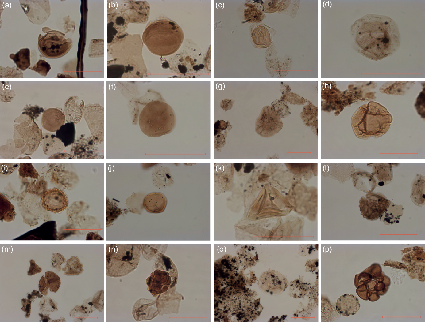
Fig. 12. Microphotographs of palynomorphs from the Argiles de Châtillon Formation. (a) Classopollis OEF-19. (b) Classopollis sample OEB-17. (c) Perinopollenites sample OEB-02. (d) Perinopollenites sample OEF-19. (e) Exesipollenites sample OEF-19. (f) Exesipollenites sample OEB-21. (g) Callialasporites dampieri sample OEB-22. (h) Callialasporites dampieri sample OEB-02. (i) Cerebropollenites sample OEB-02. (j) Trilete spore sample OEB-02. (k) Gleicheniidites sample OEF-19. (l) Ischyosporites sample OEF-19. (m) Osmundacidites sample OEB-21. (n) Osmundacidites sample OEB-21. (o) Dinocyst sample OEF-10. (p) Foraminifera remains sample OEB-02. Scale bars = 50 µm.
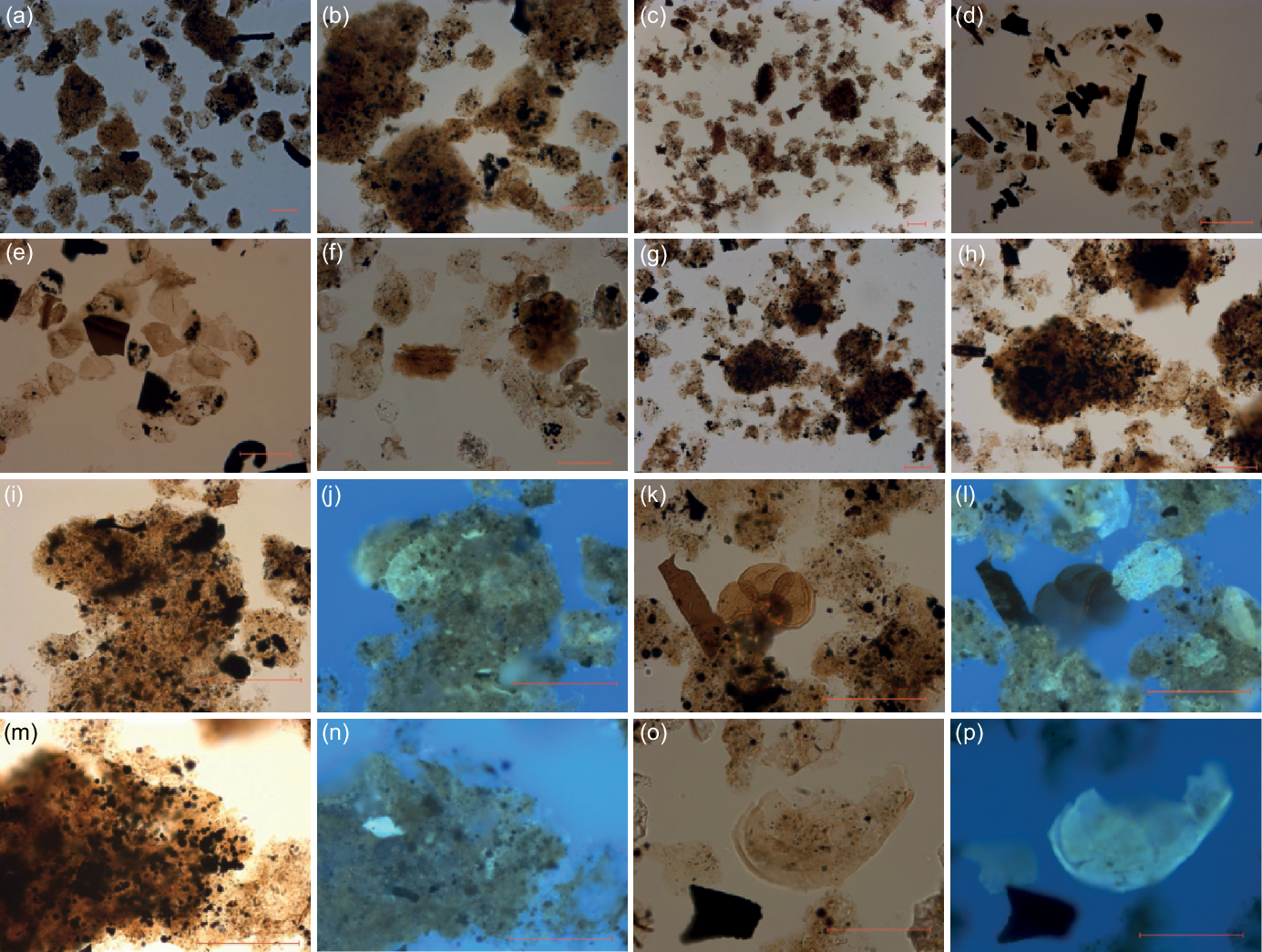
Fig. 13. Microphotographs of palynomorphs from the Argiles de Châtillon Formation. (a) Palynofacies from the lower OM-rich interval (sample OEB-03) showing dominant AOM; (b) same but with higher magnification. (c) Palynofacies from the upper OM-rich interval (sample OEF-10) showing dominant AOM. (d) Palynofacies from sample OEB-12, showing abundant wood particles. (e) Palynofacies from sample OEB-19, showing abundant sporomorphs. (f) Palynofacies from sample OEF-13 with a foraminiferal organic lining. (g) Palynofacies from sample OEF-03, showing heavy AOM. (h) Heavy AOM particle from sample OEF-03. (i) AOM particle from sample OEB-03; (j) the same AOM particle with incident UV light, showing an acritarch inside the particle. (k) Palynofacies from the lower OM-rich interval (sample OEB-03); (l) the same photograph but with incident UV light, showing a previously ‘hidden’ dinoflagellate cyst. (m) AOM particle from sample OEF-03; (n) the same particle with incident UV light. (o) An unidentifiable dinoflagellate cyst from sample OEF-13; (p) the same specimen with incident UV light. Scale bars = 50 µm.

Fig. 14. Upper: Correlation of TOC and climate trends in clay mineral assemblages (kaolinite/illite and kaolinite/illite–smectite) of Tribovillard et al. (Reference Tribovillard, Koched, Baudin, Adatte, Delattre, Abraham and Ferry2019) for the Cap de la Crèche section. There is a clear large-scale positive correlation visible between TOC and humidity. Lower: Large-scale shift from humid climate below the sequence boundary to arid climate above the sequence boundary in Cran du Noirda. Note the higher values for the clay mineral ratios compared to those in Cap de la Crèche. The Scitulus climate shift is located within the sequence boundary, based on observations in the Cran aux Œufs record.
In the Cran du Noirda record, there is a clear shift visible towards lower ratios around the base of the upper ACF. The large shift to lower values is indicative of a rapid shift towards a more arid climate, which we correlate to the early Tithonian climate shift that was recorded in the sporomorph dataset. For the upper ORI at Cap de la Crèche, the data show a trend towards more humid conditions with increasing TOC values. This pattern is very similar to the increase in humid sporomorph assemblages with increasing TOC in the equivalent interval in the Cran aux Œufs section.
The clay mineral record from Hatem et al. (Reference Hatem, Tribovillard, Averbuch, Bout-Roumazeilles, Trentesaux, Deconinck, Baudin and Adatte2017) shows alternations in smectite abundance on a similar 2 m scale in the upper ACF, most evident in the most proximal section of Cap Gris Nez. Our results shows that 2 m scale variability in the sporomorph distribution reflects humid–arid alternations. Climate fluctuations might have similarly influenced the clay mineral signal via climate-controlled runoff variations, with enhanced smectite in more proximal sites, closer to the source area (Hatem et al. Reference Hatem, Tribovillard, Averbuch, Bout-Roumazeilles, Trentesaux, Deconinck, Baudin and Adatte2017). The supply of clay minerals from the continent suggests runoff as a primary mechanism controlling nutrient supply. In other work, nutrient supply was also suggested as the link between clay mineral variations and matching variations in OM content on an orbital eccentricity timescale (Armstrong et al. Reference Armstrong, Wagner, Herringshaw, Farnsworth, Lunt, Harland, Imber, Loptson and Atar2016).
5.c.3. Milankovitch cycles in the ACF and KCF
In the Tithonian interval of the ACF (units V and VI), several asymmetrical, yet repetitive, trends towards increasing values of δ13Corg, TOC and AOM are observed on a 2 m scale (Fig. 9). In the lower-resolution sporomorph record, repetitive trends occur that seem to line up with the palynofacies and stable isotope trends. On the other hand, these alternations are clearly absent in units II and III (Kimmeridgian). The strong correlation between the TOC, palynofacies and sporomorph variability suggests a link between OM accumulation and climate cyclicity for the upper ACF interval. It is not uncommon to observe Milankovitch cyclicity in palynological data (e.g. Waterhouse, Reference Waterhouse1999; Bonis et al. Reference Bonis, Ruhl and Kürschner2010). Besides, similar-scale cyclic variations have been described in the literature for the ACF and KCF, although with varying interpretations on the duration and underlying mechanism (Herbin et al. Reference Herbin, Fernandez-Martinez, Geyssant, Albani, Deconinck, Proust, Colbeaux and Vidier1995; Waterhouse, Reference Waterhouse, House and Gale1995, Reference Waterhouse1999; Weedon et al. Reference Weedon, Jenkyns, Coe and Hesselbo1999, Reference Weedon, Coe and Gallois2004; Armstrong et al. Reference Armstrong, Wagner, Herringshaw, Farnsworth, Lunt, Harland, Imber, Loptson and Atar2016). For example, Waterhouse (Reference Waterhouse1999) observed palynofacies cycles of 60–70 cm and 30–40 cm in the ACF. The ratio between these cycles suggest obliquity and precession control. It supports a roughly 100 kyr eccentricity control for the 2 m scale alternations in the ACF.
The absolute age control on the duration of the Elegans Zone is rather weak, but is in the order of 0.2–0.5 Myr (Weedon et al. Reference Weedon, Coe and Gallois2004; Ogg, Reference Ogg, Gradstein, Ogg and Smith2005; Huang et al. Reference Huang, Hesselbo and Hinnov2010; Hesselbo et al. Reference Hesselbo, Ogg, Ruhl, Hinnov, Huang, Gradstein, Ogg, Schmitz and Ogg2020). The presence of three 2 m scale δ13Corg shifts and TOC fluctuations suggests a roughly 100 kyr eccentricity control, in agreement with similar palynofacies cycles (e.g. Waterhouse, Reference Waterhouse, House and Gale1995). Our results thus link the variations in OM content on a 100 kyr scale to terrestrial vegetation changes that are characteristic of a changing Late Jurassic climate.
5.d. Organic matter deposition
5.d.1. Spatiotemporal variations in δ13Corg and TOC content
The stable isotope values from the Cran aux Œufs section range between −26.25 ‰ and −23.94 ‰, whereas the values for the same time interval of the KCF (Morgans-Bell et al. Reference Morgans-Bell, Coe, Hesselbo, Jenkyns, Weedon, Marshall, Tyson and Williams2001) reach more positive values, ranging between −26.34 ‰ and −22.13 ‰. For the TOC content, the same applies; the overall absolute values for the KCF are considerably higher than the values of the ACF from the Cran aux Œufs section. In addition, the TOC values of the KCF display a larger variation. Interestingly, the difference in absolute values is also observed within the smaller scale of the Boulonnais area. The absolute TOC and δ13Corg values for the Cap de la Crèche section are higher than the values of the Cran aux Œufs section (Figs 7, 8). For the TOC values, this was already noted by Herbin et al. (Reference Herbin, Fernandez-Martinez, Geyssant, Albani, Deconinck, Proust, Colbeaux and Vidier1995) and Tribovillard et al. (Reference Tribovillard, Bialkowski, Tyson, Lallier-Verges and Deconinck2001). The Cap de la Crèche section is generally considered to represent a slightly more distally marine depositional setting than the Cran aux Œufs section, and the depositional setting of the Kimmeridge Clay section is the most distally marine.
When looking at the variation of the TOC and δ13Corg values within the ACF, a conspicuous difference is noted between the Tithonian interval of the OEF subsection and the Kimmeridgian interval of the OEB subsection. A strong positive correlation between δ13Corg and TOC is recorded in units IV–VI of Tithonian age, but not in units II and III of Kimmeridgian age. A similar conclusion can be drawn from the record of the KCF, as indicated in Figure 7. Cross-plots between δ13Corg and TOC for the different ammonite stages ranging from Eudoxus to Scitulus show that the correlation between TOC and δ13Corg becomes more evident after the Kimmeridgian–Tithonian boundary. In fact, for the Eudoxus and Autissiodorensis ammonite zones the correlation is weak, whereas the R 2 for the Elegans and Scitulus zones are higher in both the Boulonnais sections and the KCF (Fig. 7d–g). A closer analysis of the δ13Corg and TOC records of the KCF (Fig. 6) shows that the positive correlation between TOC and δ13Corg starts at the base of bed group 35 (Upper Autissiodorensis, Irius), which correlates to the base of Unit IV and the base of the Tithonian. The base of the Tithonian thus marks an important shift in the geochemical signature recorded in the Wessex Basin (Fig. 7h, i).
5.d.2. Basin-wide controls on OM accumulation
Based on the similar pattern in the δ13Corg records between the ACF and KCF, it is evident that the δ13Corg record can be used to make high-resolution correlations on a regional scale, despite the variations in absolute values (Figs 6, 8). The stable isotope record from the Boulonnais area shows great similarities to that of the KCF, and it is therefore considered that both records were controlled by the same (basin-scale) mechanism. In fact, δ13Corg correlations by Turner et al. (Reference Turner, Batenburg, Gradstein and Gale2019) showed that a water mass exchange with the North Sea Basin existed, and this correlation can potentially even be extended north of the Greenland–Norwegian seaway. The detailed correlation between the ACF and KCF (Fig. 6) shows that in the latest Autissiodorensis and Elegans ammonite zones (Tithonian), a mechanism was in play that led to a positive correlation between TOC and δ13Corg and a cyclic pattern of the TOC curve, which was absent during the Kimmeridgian. Apparently, local factors that could have the influenced the δ13Corg signal, such a sediment supply from the hinterland, climate and vegetation, were quite comparable through the basin, as well as on a larger regional scale. However, the differences between these formations in terms of lithology, depositional setting and absolute TOC are considerable (Proust et al. Reference Proust, Deconinck, Geyssant, Herbin and Vidier1993; Herbin et al. Reference Herbin, Fernandez-Martinez, Geyssant, Albani, Deconinck, Proust, Colbeaux and Vidier1995; Morgans-Bell et al. Reference Morgans-Bell, Coe, Hesselbo, Jenkyns, Weedon, Marshall, Tyson and Williams2001; Wignall & Newton, Reference Wignall and Newton2001; Braaksma et al. Reference Braaksma, Drijkoningen, Filippidou, Kenter and Proust2006; Gallois et al. Reference Gallois, Vadet and Etches2019). Therefore, a basin-wide controlling mechanism is required to explain the enhanced accumulation of OM in the basin.
Common boundary conditions for the formation of organic-rich sediments are enhanced productivity of OM or enhanced preservation of OM. Most productivity estimates for the KCF and ACF indicate that average productivity was in both cases not increased (Tribovillard et al. Reference Tribovillard, Bialkowski, Tyson, Lallier-Verges and Deconinck2001, Reference Tribovillard, Ramdani, Trentesaux and Harris2005, Reference Tribovillard, Koched, Baudin, Adatte, Delattre, Abraham and Ferry2019; Weedon et al. Reference Weedon, Coe and Gallois2004; van Dongen et al. Reference van Dongen, Schouten and Sinninghe Damsté2006). One of the most intriguing differences is that indications for photic zone anoxia and euxinic bottom-water conditions are plentiful for the KCF (van Kaam-Peters et al. Reference van Kaam-Peters, Schouten, de Leeuw and Sinninghe Damsté1997, Reference van Kaam-Peters, Schouten, Köster and Sinninghe Damsté1998; Sælen et al. Reference Sælen, Tyson, Telnæs and Talbot2000; van Dongen et al. Reference van Dongen, Schouten and Sinninghe Damsté2006), but these indications are virtually absent for the ACF (Tribovillard et al. Reference Tribovillard, Ramdani, Trentesaux and Harris2005, Reference Tribovillard, Koched, Baudin, Adatte, Delattre, Abraham and Ferry2019; Hatem et al. Reference Hatem, Tribovillard, Averbuch, Bout-Roumazeilles, Trentesaux, Deconinck, Baudin and Adatte2017). Despite these differences, sedimentological, palynological and palaeontological evidence shows that conditions were likely not permanently fully oxic either. So, the question arises how the enhanced OM accumulation could have worked on a basin-wide scale, by assuming a mechanism that can be applied also under predominant oxic conditions that are generally not prone to OM enrichment.
5.d.3. Preservation of OM via sulfurization of carbohydrates
The positive correlation between TOC and δ13Corg has been observed previously in the lower Tithonian of the KCF from the Wessex Basin (Huc et al. Reference Huc, Lallier-Vergès, Bertrand, Carpentier, Hollander, Whelan and Farrington1992; Sinninghe Damsté et al. Reference Sinninghe Damsté, Kok, Köster and Schouten1998; van Kaam-Peters et al. Reference van Kaam-Peters, Schouten, Köster and Sinninghe Damsté1998; Sælen et al. Reference Sælen, Tyson, Telnæs and Talbot2000; Morgans-Bell et al. Reference Morgans-Bell, Coe, Hesselbo, Jenkyns, Weedon, Marshall, Tyson and Williams2001; van Dongen et al. Reference van Dongen, Schouten and Sinninghe Damsté2006; Fig. 7) and the Yorkshire basin (Atar et al. Reference Atar, März, Aplin, Dellwig, Herringshaw, Lamoureux-Var, Leng, Schnetger and Wagner2019). Such correlation has been ascribed to the early sulfurization of carbohydrates (Sinninghe Damsté et al. Reference Sinninghe Damsté, Kok, Köster and Schouten1998; van Kaam-Peters et al. Reference van Kaam-Peters, Schouten, Köster and Sinninghe Damsté1998; van Dongen et al. Reference van Dongen, Schouten and Sinninghe Damsté2006). In most environments, carbohydrates are rapidly remineralized and therefore contribute to a very small proportion of the OM preserved in sediments. However, carbohydrates are highly reactive towards sulfides (Kok et al. Reference Kok, Schouten and Damsté2000). Free sulfides are mostly formed in the sediment by organoclastic sulfate-reduction and sulfate-driven anaerobic oxidation of methane. Sulfate-reduction reactions can take place both in the sediment and in the water column (Raven et al. Reference Raven, Fike, Gomes, Webb, Bradley and McClelland2018). In the presence of free sulfides, carbohydrates cross-link via the formation of sulfide bonds, or incorporate sulfur, and thus become more resistant to remineralization. This abiotic reaction of OM with sulfides, which also affects lipids, is called sulfurization (Sinninghe Damsté & De Leeuw, Reference Sinninghe Damsté and De Leeuw1990). The δ13Corg signature of carbohydrates is estimated to be 4–10 ‰ heavier than that of lipids (Tyson, Reference Tyson1995; Sinninghe Damsté et al. Reference Sinninghe Damsté, Kok, Köster and Schouten1998), which explains why varying amounts of preserved carbohydrates may result in δ13Corg shifts of up to 6 ‰. Since carbohydrates are also rich in hydrogen, early sulfurization of carbohydrates contributes to the preservation of high amounts of hydrogen-rich OM. This leads to the general correlation of TOC, HI and δ13Corg values as observed in the KCF.
Based on the positive correlation between TOC, organic sulfur and HI, Tribovillard et al. (Reference Tribovillard, Bialkowski, Tyson, Lallier-Verges and Deconinck2001, Reference Tribovillard, Koched, Baudin, Adatte, Delattre, Abraham and Ferry2019) demonstrated that the OM of the ORIs from the upper ACF was sulfurized. The observed correlation between TOC and sulfurized OM is similar to what was described for the KCF (Huc et al. Reference Huc, Lallier-Vergès, Bertrand, Carpentier, Hollander, Whelan and Farrington1992; van Kaam-Peters et al. Reference van Kaam-Peters, Schouten, de Leeuw and Sinninghe Damsté1997, Reference van Kaam-Peters, Schouten, Köster and Sinninghe Damsté1998). By analogy with the KCF, we propose that the correlation between AOM, TOC, HI and δ13Corg values observed in the Tithonian (units IV–VII) of the ACF results more specifically from the early sulfurization of carbohydrates.
It is important to realize that such large shifts in δ13Corg, up to 6 ‰, cannot be achieved by a change in the ratio between terrestrial and marine-derived kerogen alone (see discussion in Atar et al. Reference Atar, März, Aplin, Dellwig, Herringshaw, Lamoureux-Var, Leng, Schnetger and Wagner2019). In the Jurassic, marine type II OM had an average δ13Corg value of −28 ‰ (Tyson, Reference Tyson1995; van Dongen et al. Reference van Dongen, Schouten and Sinninghe Damsté2006). Type III terrestrial OM had a δ13Corg signature ranging between −22 ‰ and −25 ‰ (Tyson, Reference Tyson1995; Pearce et al. Reference Pearce, Hesselbo and Coe2005; van Dongen et al. Reference van Dongen, Schouten and Sinninghe Damsté2006). The difference in δ13Corg of these kerogens implies that varying amounts can account for 3 ‰ at most (Tyson, Reference Tyson1995; van Dongen et al. Reference van Dongen, Schouten and Sinninghe Damsté2006). The Jurassic type III OM had a more positive δ13Corg signature than that of type II OM. This is in contrast with its present-day signature, which is more negative than type II OM. Quaternary δ13Corg values for type III OM (Leng & Lewis, Reference Leng, Lewis, Weckström, Saunders, Gell and Skilbeck2017) cannot be safely extrapolated to be used as a marine–terrestrial proxy for the Mesozoic. Furthermore, OM with a low HI and high oxygen index, plotting as type III OM and generally corresponding to terrestrial OM, can in fact alternatively correspond to altered type II marine OM (Hare et al. Reference Hare, Kuzyk, Macdonald, Sanei, Barber, Stern and Wang2014). In addition, the terrestrial contribution to the total OM is weak in both the KCF (Tyson, Reference Tyson, Batten and Keen1989; Tribovillard et al. Reference Tribovillard, Desprairies, Lallier-Verges, Bertrand, Moureau, Ramdani and Ramanampisoa1994; Van Kaam-Peters et al. Reference van Kaam-Peters, Schouten, Köster and Sinninghe Damsté1998; Turner et al. Reference Turner, Batenburg, Gradstein and Gale2019) and the ACF, where it is mostly dominated by marine AOM and the contribution of terrestrial OM to the palynofacies and palynomorphs rarely exceeds 35 % (Fig. 8). This implies that the δ13Corg signature is unlikely to be influenced significantly by changes in the source of the OM alone.
A remarkable outcome of this study is thus that during Tithonian time, the apparently eccentricity-driven process of selective preservation of OM via the sulfurization of carbohydrates acts simultaneously in the basin centre (southern England) as well as in the more marginal areas of the basin (Boulonnais), as indicated by the correlation based on stable isotopes (Fig. 6).
5.e. Depositional model: climate controls on OM deposition in the ACF
The present study shows that there are two ORIs in the ACF that formed in contrasting settings, which agrees with the previous work of Tribovillard et al. (Reference Tribovillard, Koched, Baudin, Adatte, Delattre, Abraham and Ferry2019). The differences between the two ORIs are reflected in the palynological results and δ13Corg-to-TOC correlations. The lower ORI is thinner, has sharply defined boundaries, shows less variation in AOM content and reaches higher TOC contents. The lowest abundance of dinoflagellate cysts in the interval with highest TOC contents points towards moderate stratification, suggesting that preservation played an important role in the development of the lower ORI in the ACF, in agreement with redox-sensitive trace elements of Tribovillard et al. (Reference Tribovillard, Ramdani, Trentesaux and Harris2005, Reference Tribovillard, Koched, Baudin, Adatte, Delattre, Abraham and Ferry2019). The deposition occurred under stable, cooler and more humid climate, during rising and high relative sea level.
The upper black shales have formed under contrasting conditions. They were deposited after a climate shift to warmer and more arid conditions in early Tithonian time, which is also documented in other parts of NW Europe (Abbink et al. Reference Abbink1998; Hesselbo et al. Reference Hesselbo, Deconinck, Huggett and Morgans-Bell2009). There is a clear positive correlation between TOC and δ13Corg. Here, there is no strong palynological evidence for stratification of the water column, in agreement with the trace-element analysis of Tribovillard et al. (Reference Tribovillard, Ramdani, Trentesaux and Harris2005, Reference Tribovillard, Koched, Baudin, Adatte, Delattre, Abraham and Ferry2019). Despite this, the absence of bioturbation in the paper shale intervals and the presence of solely hypoxic foraminifera assemblages (Colpaert et al. Reference Colpaert, Nikitenko, Danelian, Elena and Igor2021) points in the direction of scarce benthic life and the (temporary) absence of fully oxygenized conditions. Under these circumstances, sulfurization of OM, in particular carbohydrates, took place, as evident from the positive correlation between TOC and δ13Corg. This ORI is thicker but shows subordinate variations on a 2 m scale. AOM and TOC content are likely controlled by the 100 kyr eccentricity cycle that controls alternations between more humid and more arid phases, reflected in the sporomorph assemblage and the clay mineral ratios. An eccentricity-modulated shift and expansion of the subtropical Hadley Cell was recently hypothesized to have affected the Late Jurassic climate, resulting in alternating humid and arid climate conditions (Armstrong et al. Reference Armstrong, Wagner, Herringshaw, Farnsworth, Lunt, Harland, Imber, Loptson and Atar2016; Colombié et al. Reference Colombié, Carcel, Lécuyer, Ruffel and Schnyder2018; Atar et al. Reference Atar, März, Aplin, Dellwig, Herringshaw, Lamoureux-Var, Leng, Schnetger and Wagner2019). According to these model simulations, monsoonal conditions, an intensified hydrological cycle with more storminess, more continental weathering and increased runoff occurred during the humid climate conditions.
Our results show that under the most humid phases of these overall arid climate conditions, sulfurization of carbohydrates was the dominant control on OM preservation. There are several studies where climate has been described to affect the sulfurization and preservation of OM (van Kaam-Peters et al. Reference van Kaam-Peters, Schouten, Köster and Sinninghe Damsté1998; Riboulleau et al. Reference Riboulleau, Baudin, Deconinck, Derenne, Largeau and Tribovillard2003; Atar et al. Reference Atar, März, Aplin, Dellwig, Herringshaw, Lamoureux-Var, Leng, Schnetger and Wagner2019). Iron supply is a key factor in sulfurization (Hartgers et al. Reference Hartgers, Lopez, Sinninghe Damsté, Reiss, Maxwell and Grimalt1997; Tribovillard et al. Reference Tribovillard, Hatem, Averbuch, Barbecot, Bout-Roumazeilles and Trentesaux2015; Shawar et al. Reference Shawar, Halevy, Said-Ahmad, Feinstein, Boyko, Kamyshny and Amrani2018; Raven et al. Reference Raven, Keil and Webb2021). As proposed for the KCF, the availability of reactive iron likely depends on changing climate, probably driven by Milankovitch cycles, which can have a large impact on the amount of sulfurization via the supply of reactive iron from the continent (aeolian dust, runoff) (van Kaam-Peters et al. Reference van Kaam-Peters, Schouten, Köster and Sinninghe Damsté1998). A similar link between increasing aridity, humid–arid alternations and OM preservation during Late Jurassic time was recorded by Riboulleau et al. (Reference Riboulleau, Baudin, Deconinck, Derenne, Largeau and Tribovillard2003). Productivity was increased as a consequence of both aeolian and fluvial nutrient supply, combined with enhanced mixing during storms. The high primary productivity increased the oxygen demand, leading to anoxic conditions in the sediment, and less efficient reoxygenation during fair-weather periods.
Based on the similarity with these examples, we propose a possible model whereby the large-scale shift to a more arid and dry climate in Tithonian time triggered eccentricity-controlled humid–arid alternations, and the onset of sulfurization as the dominant control on OM preservation in these humid periods (Fig. 15). During the most humid phases, induced by the eccentricity-modulated shift and expansion of the subtropical Hadley Cell, monsoonal conditions and an intensified hydrological cycle increased continental weathering. The terrigenous material (smectite, Fe, nutrients) was efficiently transferred to the sea because of increased runoff (Armstrong et al. Reference Armstrong, Wagner, Herringshaw, Farnsworth, Lunt, Harland, Imber, Loptson and Atar2016; Colombié et al. Reference Colombié, Carcel, Lécuyer, Ruffel and Schnyder2018; Atar et al. Reference Atar, März, Aplin, Dellwig, Herringshaw, Lamoureux-Var, Leng, Schnetger and Wagner2019). This input of nutrients promoted primary productivity in the basin. As sulfurized OM was abundant in the humid intervals in the Tithonian, there should have been a (relative) reactive iron shortage (Tribovillard et al. Reference Tribovillard, Averbuch, Bialkowski and Deconinck2002). The balance between aeolian and fluvial iron supply and consumption through iron sulfide precipitation can be subtle; small changes in primary productivity can drive large changes in OM preservation in environments near the redox threshold (Raven et al. Reference Raven, Fike, Gomes, Webb, Bradley and McClelland2018). Iron limitation can occur owing to high production of reduced sulfur in the sediment, induced by high inputs of OM and high sulfate-reduction rates (Tribovillard et al. Reference Tribovillard, Desprairies, Lallier-Verges, Bertrand, Moureau, Ramdani and Ramanampisoa1994; Riboulleau et al. Reference Riboulleau, Baudin, Deconinck, Derenne, Largeau and Tribovillard2003). If OM supply increases and fosters sulfate-reduction reactions, the created sulfide can react with iron, while an excess of free sulfides can react with OM. Thus, a higher flux of OM leads to oxygen consumption in the sediment, favouring sulfurization of carbohydrates. Nevertheless, the increased storminess leads to the recurrent mixing of the water column, so that the upper sediment is never fully anoxic, at least in the marginal part of the basin. In the more distal setting, the basin is deeper, so that even if storms are present, the water column might not be entirely mixed. Anoxia of the sediment and possibly water column can develop better, leading to even better preservation of OM.

Fig. 15. Depositional model for the ACF and KCF, explaining the (climate-controlled) mechanisms behind organic matter (OM) enrichment in the Kimmeridgian and Tithonian, and the process leading to OM sulfurization under a humid climate. The humid–arid alternations affected OM distribution on a basin-wide scale, whereas the ventilation caused by storminess resulted in oxygenated conditions in the proximal domain. PP – primary productivity; TOC – total organic carbon.
Independent of how exactly climate drives the sulfurization of OM, different mechanisms characterize OM accumulation in the Kimmeridgian versus the Tithonian. The eccentricity-controlled humid–arid alternations were initiated during Tithonian time, simultaneously with and potentially linked to the aridification of the NW European continent. This regional, climate-driven mechanism is recorded in both the distal facies of the KCF as well as the proximal facies of the ACF of Tithonian age.
6. Conclusions
Palynological, TOC and δ13Corg analyses were combined to study the OM distribution in relation to palaeoclimate for the Kimmeridgian–Tithonian interval of the ACF from the Boulonnais area. The ACF contains two intervals with elevated TOC, one in the uppermost Kimmeridgian, corresponding to the lower part of the Autissiodorensis ammonite Zone, and one in the lowermost Tithonian, corresponding to the upper Autissiodorensis (Irius) and Elegans ammonite zones. Because the ACF was deposited in a shallow-marine setting, the acquired quantitative pollen and spore record is considered to reflect actual changes in vegetation patterns that can be used as a proxy for palaeoclimate. The climate-driven changes in terrestrial vegetation are identified in the shallow-marine domain and are correlated to a more distal marine setting. The pollen and spore record of the ACF reveals a change towards warmer and more arid climate conditions around the Kimmeridgian–Tithonian boundary. Superposed on the large-scale climate trend, small-scale cycles observed in the palynological record of the upper ACF were interpreted to reflect eccentricity-driven increases in humidity and match alternations in OM content, TOC and δ13Corg. Parallel to the palynological record, a high-resolution δ13Corg record was established that allows direct comparison and correlation of the proximal mudstones from the ACF to the distal mudstones of the KCF. The detailed correlation leads to the conclusion that the underlying mechanism that dictated the trends in TOC and δ13Corg of the KCF is also applicable to the shallower marine ACF record, albeit in a more moderate fashion. The cyclic increases in TOC and δ13Corg reflect sulfurization of carbohydrates, which we related to the eccentricity-driven humid–arid alternations. The ORI from the uppermost Kimmeridgian Autissiodorensis Zone does not exhibit this relationship: the TOC values and the δ13Corg do not show a correlation and small-scale climate trends are absent in the palynological record. Here, OM accumulation is thus solely related to stratification of the water column. In conclusion, an important change occurred in the NW European climate across the Kimmeridgian–Tithonian boundary, towards warmer and more arid conditions with superimposed eccentricity-controlled changes in humidity. The latter appears to be a crucial driver for sulfurization of OM, which controlled OM accumulation in the Tithonian period on a basin-wide scale.
Supplementary material
To view supplementary material for this article, please visit https://doi.org/10.1017/S0016756822001121
Acknowledgements
This work was financially supported by TNO Geological Survey of the Netherlands. We thank Nico Janssen, Sander Houben and Bart van der Kwaak for scientific discussions and/or assistance during field work. We thank Andrew Aplin and one anonymous reviewer for their comments that improved the manuscript.
Conflict of interest
None.


 Open access