


1. Introduction
It is well known that interaction of two oblique shock waves in a steady two-dimensional flow can be regular or irregular, depending on the flow Mach number and angles of the incident shock waves (Ben-Dor Reference Ben-Dor2007). In a regular reflection, two reflected shock waves and a slip surface (if the angles of incidence are not identical) emanate from the reflection point. In an irregular reflection, two triple points located at a certain distance from each other are formed. Each triple point is the point of meeting of the incident and reflected shock waves, as well as another shock wave called the Mach stem. A slip surface also emanates from each triple point. The Mach stem connects two triple points, and there is a closed zone of a subsonic flow behind it.
Such shock wave configurations can be analysed theoretically with the inviscid Euler equations. Under this approximation, a shock wave is a discontinuity without internal structure. It follows from the mass, momentum and energy conservation laws that the gas-dynamic variables on both sides of the discontinuity satisfy certain algebraic relations known as the Rankine–Hugoniot relations. With the Rankine–Hugoniot relations for all shock waves, it is possible to determine local slopes of the discontinuities at the points of their intersection and the flow parameters behind them. The discontinuities in the near vicinity of the triple point are assumed to be planar (straight lines in the two-dimensional case). If the discontinuity curvature is taken into account, then additional expressions relating the derivatives of the gas-dynamic variables upstream and downstream of the discontinuity should be used (Adrianov, Starykh & Uskov Reference Adrianov, Starykh and Uskov1995; Emanuel Reference Emanuel2013; Mölder Reference Mölder2016). The above-described approach has been employed to predict the parameters of two-shock and three-shock configurations formed in the regular and irregular reflections, respectively (von Neumann Reference von Neumann1943).
Further investigations have shown that theoretical predictions agree well with experimental data only for reflection of sufficiently strong shock waves where the free-stream Mach number  $M_\infty$ is approximately 3 or higher (referred to hereinafter as the strong reflection). As for shock wave configurations formed due to interaction of weaker shock waves (referred to below as the weak reflection), there is a range of parameters where three-shock configurations are theoretically impossible, but an irregular reflection with clearly visible triple points is observed in experiments. This contradiction between theory and experiments is known as the von Neumann paradox or the triple point paradox.
Trying to resolve this paradox within the model of an inviscid non-heat-conducting gas, Guderley proposed a four-wave model (Guderley Reference Guderley1947, Reference Guderley1962). This model implies that a centred expansion wave additionally emanates from the shock wave intersection point in the irregular reflection, and a local supersonic region is adjacent to this wave. The additional wave allows one to find the solution of the system of conservation laws. The first confirmation of this model was obtained only half a century later by solving the Euler equations numerically (Vasilev & Kraiko Reference Vasilev and Kraiko1999). Further investigations (Hunter & Brio Reference Hunter and Brio2000; Tesdall & Hunter Reference Tesdall and Hunter2002; Hunter & Tesdall Reference Hunter and Tesdall2004; Tesdall, Sanders & Keyfitz Reference Tesdall, Sanders and Keyfitz2007, Reference Tesdall, Sanders and Keyfitz2008; Defina, Susin & Viero Reference Defina, Susin and Viero2008a; Defina, Viero & Susin Reference Defina, Viero and Susin2008b; Vasilev & Olhovskiy Reference Vasilev and Olhovskiy2009; Tesdall, Sanders & Popivanov Reference Tesdall, Sanders and Popivanov2015; Vasil'ev Reference Vasil'ev2016) showed that, depending on problem parameters, configurations formed due to interaction of weak shock waves can have even more complicated structures and contain additional elements of small size. The experiments by Skews & Ashworth (Reference Skews and Ashworth2005) and Skews, Li & Paton (Reference Skews, Li and Paton2009) performed in a large shock tube revealed the existence of a configuration similar to that predicted by Guderley and observed in the inviscid studies mentioned above. However, the size of local supersonic regions observed in those experiments was greater by an order of magnitude than that predicted by numerical solutions of the Euler equations.
As the theoretical inviscid solution contains structures that are very small in comparison to the characteristic length scales of the problem, such as the Mach stem length, the question about possible roles of viscosity and heat conduction arises. As is well known, if viscosity and heat conduction are taken into account, then the discontinuity transforms into the shock transition zone of finite thickness. A steady solution of one-dimensional Navier–Stokes equations for the internal structure of a normal shock wave can be easily obtained numerically (Gilbarg & Paolucci Reference Gilbarg and Paolucci1953). The structure of an oblique shock wave can be calculated as a superimposition of this one-dimensional normal shock solution and a uniform flow directed along the shock wave.
A comparison with the experimental data shows that the theory based on the Navier–Stokes equations provides a quantitatively correct description of the shock wave structure only for weak shock waves. Starting approximately from  $M_\infty = 2$, the molecular velocity distribution function departs from the Maxwellian equilibrium form (see e.g. Bird Reference Bird1994); hence the kinetic approach – direct numerical solution of the Boltzmann equation or the direct simulation Monte Carlo (DSMC) method (Bird Reference Bird1994) – should be employed for the shock wave structure problem (see e.g. Malkov et al. Reference Malkov, Bondar, Kokhanchik, Poleshkin and Ivanov2015).
It seems feasible to apply the Navier–Stokes equations to analysing the possible influence of dissipative effects in the shock wave reflection problem, at least as the first approximation. It should be kept in mind, however, that while the Navier–Stokes equations ensure a qualitatively correct description of the viscous shock wave structure, the shock wave thickness and the distributions of gas-dynamic parameters inside the shock wave can be quantitatively different from those predicted by the kinetic approach, especially at high free-stream Mach numbers.
The internal structure of interacting shock waves far from their intersection is described well by the one-dimensional solution mentioned above. Behind the viscous shock transition, the variables approach asymptotically the constant values predicted by the inviscid Rankine–Hugoniot relations. However, the situation is essentially different in the shock interaction region. The Rankine–Hugoniot relations do not hold exactly inside the zone of an essentially two-dimensional flow formed as a result of the interaction of oblique shock waves of finite thickness, which have their own internal structure. This fact was noticed for the first time by Sternberg (Reference Sternberg1959), who coined the term ‘non-Rankine–Hugoniot zone’ to denote the region of interaction of shock waves in the viscous flow. Later, Sichel (Reference Sichel1963) derived, for Mach numbers close to unity, a simplified system of equations to describe fluid motion in such a zone. Sakurai (Reference Sakurai1964) considered the phenomenon of the non-Rankine–Hugoniot zone and the role of viscous effects with the approximate solution of the Navier–Stokes equations. More recently, the flow field near the triple point was studied numerically by Sakurai et al. (Reference Sakurai, Tsukamoto, Khotyanovsky and Ivanov2011) and compared with the developed analytical model, which takes viscous effects into account.
An attempt was made in the experiments of Siegenthaler & Madhani (Reference Siegenthaler and Madhani1998) to detect the differences in the flow parameters in the weak reflection from those predicted by the classical inviscid model, and the authors declared that such differences were indeed observed. Later, the authors tried to explain the results obtained by modifying the Rankine–Hugoniot relations in such a way that the total enthalpy of the flow behind the shock wave was not equal to the free-stream total enthalpy (Siegenthaler & Madhani Reference Siegenthaler and Madhani2001).
Based on the numerical solution of the Navier–Stokes equations and DSMC simulations, the non-Rankine–Hugoniot zone was observed in low-Reynolds-number flows for both the weak and strong reflections (Khotyanovsky et al. Reference Khotyanovsky, Bondar, Kudryavtsev, Shoev and Ivanov2009; Ivanov et al. Reference Ivanov, Bondar, Khotyanovsky, Kudryavtsev and Shoev2010a; Chen, Zhang & Liu Reference Chen, Zhang and Liu2016; Liu et al. Reference Liu, Chen, Zhang and Liu2019). Similar deviations from the theoretical solution were also reported by Ben-Dor, Takayama & Needham (Reference Ben-Dor, Takayama and Needham1987), who solved the Euler equations with a shock-capturing scheme in order to study unsteady reflection of the shock wave from a wedge. However, the deviations in Ben-Dor et al. (Reference Ben-Dor, Takayama and Needham1987) were induced not by physical viscosity but by numerical dissipation inherent in any shock-capturing scheme.
Sternberg (Reference Sternberg1959) assumed that the von Neumann paradox is an example of the flow where the viscous solution does not approach the inviscid solution as the Reynolds number tends to infinity. Generally speaking, examples of such flows are known. One example is the Jeffery–Hamel flow between two plane diverging walls (Jeffery Reference Jeffery1915; Hamel Reference Hamel1916). In this case, the solution of the Navier–Stokes equations does not approach any certain limit as  $\textit {Re} \to \infty$, and does not converge to the inviscid solution.
However, Ivanov et al. (Reference Ivanov, Shoev, Khotyanovsky, Bondar and Kudryavtsev2012) demonstrated by solving the Navier–Stokes equations numerically that in the case of the von Neumann paradox, the non-Rankine–Hugoniot zone size decreases and the values of the flow variables downstream from this zone become closer and closer to the inviscid four-wave solution of Guderley (Reference Guderley1947, Reference Guderley1962) as the Reynolds number increases. At the same time, the numerical results revealed that viscosity significantly affects the flow even at very high Reynolds numbers (up to  $\textit {Re} \approx 10^9$). It can be concluded that under conditions observed in nature or real technical systems, the flow field near the interaction region of weak shock waves may be quite far from the theoretical inviscid solution, though it is expected to approach the latter with increasing Reynolds number.
For the strong reflection, the passage from the viscous solution to the inviscid-limit three-shock solution has not been investigated. Such a study has not been conducted for the weak reflection either in the case where the inviscid theory predicts the existence of a three-shock configuration, i.e. outside the range of the von Neumann paradox conditions. The goal of the present paper is to fill this gap by performing such a numerical investigation for the irregular shock wave reflection in steady flows. The study focuses mainly on the strong reflection, but the case of weak reflection outside the von Neumann paradox conditions is also addressed. The flow is modelled with the Navier–Stokes equations. Despite the fact that the length scales of interest are comparable with the shock wave thickness, previous studies (Khotyanovsky et al. Reference Khotyanovsky, Bondar, Kudryavtsev, Shoev and Ivanov2009; Ivanov et al. Reference Ivanov, Bondar, Khotyanovsky, Kudryavtsev and Shoev2010a) demonstrated clearly that the Navier–Stokes solution for the shock interaction region agrees well with DSMC results for both strong and weak reflections.
The paper is organised in the following way. Section 2 describes the problem formulation. The procedure for constructing the inviscid three-shock solution with the shock polar technique is discussed in § 3. The numerical method used for investigating the viscous structure of the flow near the triple point is presented in § 4. The results of the numerical study of the strong reflection are given in § 5, while the results for weak shock waves are reported in § 6. Section 7 contains a discussion of the results, and conclusions are formulated in § 8. Appendix A is provided to demonstrate that at the Prandtl number  $\textit {Pr} = 3/4$, the total enthalpy is constant everywhere inside the planar shock wave front (shock transition zone). This property of the Navier–Stokes equations is used in the paper when discussing the numerical results.
2. Problem formulation
We consider a steady flow between two symmetrically arranged wedges immersed in a uniform supersonic stream. The flow field is also assumed to be symmetric. In the present study, we consider the flow field portion located above the symmetry plane as shown in figure 1. The wedge with the windward side  $w$ generates the incident shock wave. For a fixed specific heats ratio $\gamma$, various shock wave configurations can be formed depending on the free-stream Mach number $M_\infty$, the wedge inclination angle $\theta _w$, and the distance between the wedge trailing edge and the symmetry plane $g$. The resultant configuration consists of the incident (IS) and reflected (RS) shock waves, the Mach stem (MS), and the shear layer (SL). An expansion fan (EF) emanates from the trailing edge of the wedge (point 3) and interacts with the reflected shock wave and the shear layer. Owing to this interaction, the shear layer becomes curved, and a virtual nozzle is formed (Hornung & Robinson Reference Hornung and Robinson1982). The subsonic flow behind the Mach stem enters the converging part of the virtual nozzle. The flow becomes supersonic passing through the throat cross-section, and accelerates further in the diverging part of the virtual nozzle.

Figure 1. Flow pattern and computational domain for the strong reflection.
The flow of a monatomic gas with the ratio of specific heats  $\gamma =5/3$ is studied numerically in the present work. Two cases are considered: the strong and weak reflection. In the strong reflection, the free-stream Mach number is $M_\infty =4$, and the wedge angle is $\theta _w=25^\circ$. The distance between the trailing edge of the wedge and the symmetry plane $g=0.75w$ is chosen in such a way that the expansion fan EF does not interact with the incident shock wave and meets the reflected shock wave sufficiently far from the region of shock wave interaction. In the weak reflection, $M_\infty =1.7$, $\theta _w=8.5^\circ$ and $g=0.756 w$. Numerical simulations are performed at different values of the Reynolds number $\textit {Re}_w$ calculated using the free-stream parameters and the length of the inclined part of the wedge $w$; the latter is used hereinafter as the reference scale. A power-law dependence of dynamic viscosity on temperature $\mu = T^{\omega }$ with $\omega =0.81$ in accordance with available data for argon (Bird Reference Bird1994) is assumed. The Knudsen number $Kn_w$ based on the free-stream parameters and the length of the wedge for variable hard sphere molecules can be calculated as (Bird Reference Bird1994)
 \begin{equation} Kn_w = \frac{2 (5 - 2\omega) (7 - 2\omega)}{15 {\rm \pi}^{1/2}}{\left(\frac{\gamma}{2}\right)^{1/2}} \frac{M_\infty}{\textit{Re}_w}. \end{equation}
The range of the Reynolds numbers  $\textit {Re}_w$ is considered from $10^4$ to $10^8$ for the strong reflection, and from $4 \times 10^3$ to $2 \times 10^8$ for the weak reflection. It corresponds to the range of the Knudsen numbers $Kn_w$ from approximately $5 \times 10^{-4}$ to $5 \times 10^{-8}$ for the strong reflection, and from $5.3 \times 10^{-4}$ to $10^{-8}$ for the weak reflection.
3. Inviscid three-shock solution
A shock polar of the incident shock wave (I-polar, figure 2) is the locus of all possible combinations of the flow deflection angle  $\theta$ and the ratio of gas pressure to its free-stream value $p/p_\infty$ behind all possible oblique shock waves at fixed $M_\infty$ and $\gamma$. Point $(0, 1)$ corresponds to the free stream, and point A to the parameters behind the Mach stem in the symmetry line (an example of the strong reflection is illustrated in figure 1).

Figure 2. Shock polars: (a) strong reflection,  $M_\infty =4$, $\gamma =5/3$ and $\theta _w=25^\circ$; (b) weak reflection, $M_\infty =1.7$, $\gamma =5/3$ and $\theta _w=8.5^\circ$.
A shock polar of the reflected shock wave (R-polar) is plotted from point D corresponding to the flow parameters behind the incident shock wave (see point D in figure 1). The intersection point of the I-polar and the R-polar corresponds to the flow parameters behind the intersection point of the shock waves IS, RS and MS (triple point; see figure 1). Hereinafter, the term ‘triple point’ is used for both inviscid and viscous flows for simplicity (though, strictly speaking, there is a finite shock interaction region in the viscous case). In the inviscid case, the pressure and the flow deflection angle do not change across the slip line emanating from the triple point; therefore points B and C in the flow field correspond to the same point in the  $(\theta, p/p_\infty )$ plane. After determining the flow deflection angle and the pressure at point B(C), one can apply the Rankine–Hugoniot relations to find the slopes of the shock waves and the slip line at the triple point, and also the flow parameters behind them. The combination of all these parameters will be referred to below as the three-shock solution (Ben-Dor Reference Ben-Dor2007).
When moving along the Mach stem from the symmetry plane to the triple point (segment AB in figure 1), the slope of the Mach stem MS changes from  $90^\circ$ to the angle predicted by the three-shock solution. The flow parameters behind the Mach stem also change when passing over the segment AB of the I-polar. The pressure and the deflection angle do not change across the slip line. In further motion upwards along the reflected shock wave, the flow parameters behind this wave should lie on the R-polar. The above-described inviscid solution implies that all three shock waves are infinitely thin and intersect each other at one point. This assumption allows one to use the classical Rankine–Hugoniot relations on oblique shock waves. Obviously, the above-mentioned non-Rankine–Hugoniot zone does not exist in this inviscid formulation.
The inviscid solutions presented in figure 2 are constructed for two principally different cases, namely, the strong (figure 2a) and weak (figure 2b) reflections. From the physical perspective, the main difference between the strong and weak reflections is that the flow behind the reflected shock wave is usually supersonic in the former case (point B(C) lies on the lower ‘weak’ branch of the R-polar; see figure 2a), while it is usually subsonic in the latter case (point B(C) lies on the upper ‘strong’ branch of the R-polar; see figure 2b). The free-stream Mach numbers ( $M_\infty =4$ and $M_\infty =1.7$) are the same as in our previous studies of the strong (Khotyanovsky et al. Reference Khotyanovsky, Bondar, Kudryavtsev, Shoev and Ivanov2009) and weak (Ivanov et al. Reference Ivanov, Bondar, Khotyanovsky, Kudryavtsev and Shoev2010a) irregular reflections. The wedge angles are chosen in such a way that the shock polar intersection points are on the left of point D in both cases. As was observed in the previous studies, the mutual arrangement of the shock polars defines the qualitative character of the flow. Variations of the free-stream parameters, the wedge angle and the ratio of specific heats may induce only quantitative changes (Ivanov et al. Reference Ivanov, Bondar, Khotyanovsky, Kudryavtsev and Shoev2010a; Chen et al. Reference Chen, Zhang and Liu2016; Liu et al. Reference Liu, Chen, Zhang and Liu2019) and therefore are not considered in the present work.
4. Numerical procedure
Numerical simulation of the Mach reflection is performed by solving the Navier–Stokes equations with the CFS solver developed at ITAM SB RAS. This solver was used earlier by Khotyanovsky et al. (Reference Khotyanovsky, Bondar, Kudryavtsev, Shoev and Ivanov2009) and Ivanov et al. (Reference Ivanov, Bondar, Khotyanovsky, Kudryavtsev and Shoev2010a) for simulating irregular reflection at low Reynolds numbers, together with the SMILE software system (Ivanov, Markelov & Gimelshein Reference Ivanov, Markelov and Gimelshein1998) based on the DSMC method (Bird Reference Bird1994). The data obtained with two different approaches were found to agree well with each other. As the free-stream conditions of the present study are close to those in Khotyanovsky et al. (Reference Khotyanovsky, Bondar, Kudryavtsev, Shoev and Ivanov2009) and Ivanov et al. (Reference Ivanov, Bondar, Khotyanovsky, Kudryavtsev and Shoev2010a), no significant differences in the DSMC and Navier–Stokes results are expected (this is one of the reasons why additional DSMC computations are not performed).
The Navier–Stokes equations are solved numerically in the present study in the dimensionless form using the following dimensionless variables:
 \begin{equation} \left.\begin{gathered}
\boldsymbol{x} = (x ,y) = \frac{\boldsymbol{x}^*}{w},\quad
\boldsymbol{u} = (u, v) =
\frac{\boldsymbol{u}^*}{a^*_\infty},\quad t =
\frac{t^*a^*_\infty}{w},\quad \rho =
\frac{\rho^*}{\rho^*_\infty}, \\ p =
\frac{p^*}{\rho^*_\infty (a^*_\infty)^2},\quad T =
\frac{T^*}{T^*_\infty},\quad E = \frac{E^*}{\rho^*_\infty
(a^*_\infty)^2},\quad \mu = \frac{\mu^*}{\mu^*_\infty}.
\end{gathered}\right\}
\end{equation}
\begin{equation} \left.\begin{gathered}
\boldsymbol{x} = (x ,y) = \frac{\boldsymbol{x}^*}{w},\quad
\boldsymbol{u} = (u, v) =
\frac{\boldsymbol{u}^*}{a^*_\infty},\quad t =
\frac{t^*a^*_\infty}{w},\quad \rho =
\frac{\rho^*}{\rho^*_\infty}, \\ p =
\frac{p^*}{\rho^*_\infty (a^*_\infty)^2},\quad T =
\frac{T^*}{T^*_\infty},\quad E = \frac{E^*}{\rho^*_\infty
(a^*_\infty)^2},\quad \mu = \frac{\mu^*}{\mu^*_\infty}.
\end{gathered}\right\}
\end{equation}
Here,  $\boldsymbol {x}$ is the vector of the spatial coordinates, $w$ is the wedge length, $\boldsymbol {u}$ is the fluid velocity, $a$ is the speed of sound, $t$ is the time, $\rho$ is the density, $p$ is the pressure, $T$ is the temperature, $E$ is the total energy per unit mass, and $\mu$ is the dynamic viscosity. The dimensional quantities are marked by an asterisk, and the free-stream parameters are labelled by the subscript $\infty$.
In view of (4.1), the Navier–Stokes equations in the conservative form are
 \begin{gather} \frac{\partial {\boldsymbol{Q}}}{\partial t} + \frac{\partial {\boldsymbol{F}}}{\partial x} + \frac{\partial {\boldsymbol{G}}}{\partial y} = \frac{M_\infty}{\textit{Re}_w} \left(\frac{\partial{\boldsymbol{F}}_{\boldsymbol{v}}}{\partial x} + \frac{\partial {\boldsymbol{G}}_{\boldsymbol{v}}}{\partial y}\right), \end{gather}
 \begin{gather} \left.\begin{gathered}
{\boldsymbol{Q}} = \left(\begin{array}{@{}c@{}} \rho \\ \rho u \\
\rho v \\ E \end{array}\right),\quad {\boldsymbol{F}} =
\left(\begin{array}{@{}c@{}} \rho u \\ \rho u^2 + p \\ \rho u v
\\ (E + p) u \end{array}\right),\quad {\boldsymbol{G}} =
\left(\begin{array}{@{}c@{}} \rho v \\ \rho u v \\ \rho v^2 + p
\\ (E + p) v \end{array}\right), \\
{\boldsymbol{F}}_{\boldsymbol{v}} = \left(\begin{array}{@{}c@{}}
0 \\ \tau_{xx}\\ \tau_{xy}\\ \beta_x
\end{array}\right),\quad {\boldsymbol{G}}_{\boldsymbol{v}}
= \left(\begin{array}{@{}c@{}} 0\\ \tau_{xy}\\ \tau_{yy}\\
\beta_y \end{array}\right).
\end{gathered}\right\} \end{gather}
\begin{gather} \left.\begin{gathered}
{\boldsymbol{Q}} = \left(\begin{array}{@{}c@{}} \rho \\ \rho u \\
\rho v \\ E \end{array}\right),\quad {\boldsymbol{F}} =
\left(\begin{array}{@{}c@{}} \rho u \\ \rho u^2 + p \\ \rho u v
\\ (E + p) u \end{array}\right),\quad {\boldsymbol{G}} =
\left(\begin{array}{@{}c@{}} \rho v \\ \rho u v \\ \rho v^2 + p
\\ (E + p) v \end{array}\right), \\
{\boldsymbol{F}}_{\boldsymbol{v}} = \left(\begin{array}{@{}c@{}}
0 \\ \tau_{xx}\\ \tau_{xy}\\ \beta_x
\end{array}\right),\quad {\boldsymbol{G}}_{\boldsymbol{v}}
= \left(\begin{array}{@{}c@{}} 0\\ \tau_{xy}\\ \tau_{yy}\\
\beta_y \end{array}\right).
\end{gathered}\right\} \end{gather}
The components of the viscous stress tensor  $\tau _{ij}$ are
 \begin{gather}
\tau_{xx} = \frac{2\mu}{3}\left(2\,\frac{\partial u}{\partial x} -
\frac{\partial v}{\partial y}\right),\quad \tau_{xy} =
\mu\left(\frac{\partial u}{\partial y} + \frac{\partial
v}{\partial x}\right),\quad \tau_{yy} =
\frac{2\mu}{3}\left(2\,\frac{\partial v}{\partial y} -
\frac{\partial u}{\partial x} \right),
\end{gather}
\begin{gather}
\tau_{xx} = \frac{2\mu}{3}\left(2\,\frac{\partial u}{\partial x} -
\frac{\partial v}{\partial y}\right),\quad \tau_{xy} =
\mu\left(\frac{\partial u}{\partial y} + \frac{\partial
v}{\partial x}\right),\quad \tau_{yy} =
\frac{2\mu}{3}\left(2\,\frac{\partial v}{\partial y} -
\frac{\partial u}{\partial x} \right),
\end{gather}
while  $\beta _x$ and $\beta _y$ contain the viscous dissipation and heat flux terms:
 \begin{equation} \beta_x = u\tau_{xx} + v\tau_{xy} + \frac{\mu}{(\gamma - 1)\,\textit{Pr}}\,\frac{\partial T}{\partial x},\quad \beta_y = u\tau_{xy} + v\tau_{yy} + \frac{\mu}{(\gamma - 1)\,\textit{Pr}} \frac{\partial T}{\partial y}. \end{equation}
Here,  $\textit {Pr}$ is the constant Prandtl number equal to $2/3$ everywhere except in § 5.3.
The perfect gas law is used to close this system of equations:
 \begin{equation} p = \frac{\rho T}{\gamma}. \end{equation}
The Navier–Stokes equations are solved on a structured rectangular mesh using the fifth-order weighted essentially non-oscillatory (WENO) scheme (Jiang & Shu Reference Jiang and Shu1996) for the convective terms, the fourth-order central difference scheme (Kudryavtsev & Khotyanovsky Reference Kudryavtsev and Khotyanovsky2005) for the diffusion terms, and the second-order Runge–Kutta scheme to march in time. Time integration is performed until the steady-state solution is reached.
The computations are performed at various Reynolds numbers  $\textit {Re}_w$ using the nested-block grid refinement technique, which was applied earlier in several studies (Defina et al. Reference Defina, Susin and Viero2008a; Tesdall et al. Reference Tesdall, Sanders and Keyfitz2008; Ivanov et al. Reference Ivanov, Shoev, Khotyanovsky, Bondar and Kudryavtsev2012) for modelling flows near the triple point. The zeroth level of nesting corresponds to the rectangular domain marked as Block 0 in figure 1. The uniform free-stream supersonic flow with the Mach number $M_\infty$ is specified as the boundary condition at the left (inflow) boundary 1–2. The parameters calculated from the Rankine–Hugoniot relations behind the IS are set on the upper boundary segment 2–3, while segment 3–4 is a solid wall. Inviscid boundary conditions are imposed on segment 3–4 because the wedge boundary layer effects are not of interest for the present work. The right (outflow) boundary 4–5 is located sufficiently far downstream so that the flow is supersonic there, and all variables are extrapolated from the interior of the computational domain. The lower boundary 1–5 is the symmetry line.
In the strong reflection, the computational domain length is  $1.5w$, while its height is equal to $g = 0.75 w$. A uniform rectangular mesh in Block 0 consists of $1600\times 800$ cells. In the weak reflection, the length of the computational domain is $1.4 w$, its height is $0.756w$, and the number of cells is $2400 \times 1200$. The computation starts from the free-stream uniform flow.
The numerical solution in Block 0 allows one to resolve the internal structure of shock waves only at sufficiently low Reynolds numbers. Smaller blocks with a more and more refined grid are added consecutively to increase the resolution near the triple point at high Reynolds numbers. Each next block is entirely situated inside the previous one. As a result, the internal structure of shock waves can always be resolved using reasonable computer resources.
The first level of nesting is shown in figure 1 and denoted as Block 1. The numerical solution obtained in Block 0 is interpolated onto a new computational domain, which is Block 1. The interpolated flow field is prescribed as initial conditions for computations in Block 1. As earlier, the free-stream parameters are set on the left boundary. The boundary conditions obtained as a result of interpolation of the numerical solution in Block 0 are imposed on the upper boundary. At the supersonic parts of the lower and right boundaries, all variables are extrapolated from the interior of Block 1. At the subsonic parts of the lower and right boundaries, the pressure interpolated from Block 0 is specified, while all other variables are extrapolated from the interior of Block 1. In Block 1, the mesh is refined near the triple point, while the cell sizes on the interface between two blocks are comparable. The computation in Block 1 is continued on a finer mesh. The density contours obtained in Block 0 and Block 1 at  $\textit {Re}_w=10^4$ are shown in figure 1. A three-shock configuration consisting of the incident IS and reflected RS shock waves and the Mach stem MS is clearly visible in both cases. A slipstream emanates from the triple point; the thickness of this slipstream gradually increases in the downstream direction. The next levels of nesting are constructed consecutively in the same manner until the number of cells across the shock waves reaches 40 or more, which is sufficient for an accurate description of the flow in the region of shock wave interaction. For the maximum value of the Reynolds number $\textit {Re}_w = 10^{8}$, 17 levels of nesting are required for the adequate resolution of flow details.
Figure 3 shows the mesh and the pressure contours in Block 17 for the strong reflection at the Reynolds number  $\textit {Re}_w=10^{8}$ in coordinates normalised to $\lambda _\infty$, the mean free path of molecules in the free stream calculated with the variable hard sphere model. There are approximately 70 cells across the IS, 90 cells across the RS, and 40 cells across the MS.

Figure 3. Mesh and pressure contours in the vicinity of the shock wave intersection for the strong reflection at  $\textit {Re}_w=10^{8}$ in Block 17. Each second line of the mesh is shown.
5. Numerical results: the strong reflection
5.1. Effects of viscosity
The pressure field obtained in Block 0 at  $\textit {Re}_w=10^4$ is shown in figure 4(a). The Navier–Stokes numerical solution is compared with the shock polars in figure 4(b). The notations ‘Block 0, MS’ and ‘Block 0, RS’ are used to label the distributions of the corresponding quantities behind the Mach stem and the reflected shock wave along the lines shown in figure 4(a). The notation ‘Block 3’ refers to the distributions of parameters behind the Mach stem and the reflected shock wave near the triple point on the third – maximum for this Reynolds number – level of nesting.

Figure 4. (a) Pressure contours at  $\textit {Re}_w=10^4$. (b) Comparison of the Navier–Stokes numerical solution with the shock polars.
In accordance with the inviscid theory, the MS slope is expected to change from  $90^\circ$ at the symmetry line to the angle predicted by the three-shock solution near the triple point, when moving upwards along the MS. Correspondingly, the flow deflection angle should change from zero to the value equal to the slope of the slip line in the three-shock solution. The numerical data in figure 4 show that when moving up the Mach stem, the angle increases at first, and in the $(\theta, p/p_\infty )$ plane, the data point moves exactly along the I-polar. Further up, closer to the three-shock intersection, the data point starts to move in the opposite direction along the I-polar, so that the flow deflection angle decreases and reaches a local minimum at some point B. When it starts to increase again, the point leaves the I-polar. Now both the pressure and the flow deflection angle increase, pass through local maxima, then start to decrease, and finally reach the R-polar at point D. However, point D does not coincide with the shock polar intersection point: it corresponds to a slightly higher value of the RS slope than that predicted by the three-shock solution. During further motion along the reflected shock wave, the data point moves along the R-polar, reaches the shock polar intersection point, and remains at this point until the reflected shock wave meets the first characteristic of the expansion fan EF. Further, the pressure and the flow deflection angle decrease rapidly.
The above-described behaviour of the numerical data in the  $(\theta, p/p_\infty )$ plane is similar to what was observed previously by Khotyanovsky et al. (Reference Khotyanovsky, Bondar, Kudryavtsev, Shoev and Ivanov2009), Chen et al. (Reference Chen, Zhang and Liu2016) and Shoev & Ivanov (Reference Shoev and Ivanov2016) at low Reynolds numbers. As was noted above, similar deviations from the three-shock solution were also obtained in inviscid computations by Ben-Dor et al. (Reference Ben-Dor, Takayama and Needham1987), where they were caused by numerical viscosity inevitably present in shock-capturing schemes. In the present study, the deviations from the inviscid solution are caused by the sole influence of physical viscosity because the effects of numerical viscosity on the solution are made negligible by using sufficiently fine meshes resolving the internal structure of the shock waves. The deviation of the numerical data in Block 3 illustrates the influence of physical viscosity on the flow structure near the triple point, and confirms the existence of the non-Rankine–Hugoniot zone in the strong Mach reflection.
Let us consider the structure of this region in more detail. The numerical solution at  $\textit {Re}_w=10^4$ obtained in Block 3 with complete resolution of the internal structure of shock waves is shown in figure 5. Figure 5(a) shows the Mach number field, where the black solid lines indicate the positions of the shock waves and slip line predicted by the three-shock solution. According to the three-shock solution, the predicted values of the Mach number behind the reflected shock wave and the Mach stem are 1.15 and 0.51, respectively. The viscosity leads to a small (within 3 %) decrease in both values.

Figure 5. Comparison of the viscous numerical solution with the inviscid solution near the triple point: (a) Mach number; (b) pressure contours; (c) numerical data and shock polars in the  $(\theta, p/p_\infty )$ plane; (d) distributions of the flow deflection angle.
The pressure field is shown in figure 5(b). The inviscid three-shock solution predicts a constant-pressure region behind the triple point where  $p/p_\infty =19.56$. In the viscous case, however, the constant-pressure region behind the triple point is not observed. There is a small region near point C where the pressure is approximately 10 % higher than that predicted by the three-shock theory. Further downstream from the shock waves, the pressure decreases, but there are some differences from the three-shock predictions even at a distance of $40\unicode{x2013} 60\lambda _\infty$. The points along the dashed line in figure 5(b) correspond to the points in the $(\theta, p/p_\infty )$ plane in figure 5(c). On the segment AB, the numerical data almost coincide with the I-polar, though the polar is passed in the opposite direction in this case. Starting from point B, the numerical data deviate significantly from the shock polars, and the flow deflection angle and the pressure increase. The pressure is maximum at point C, located immediately behind the shock wave intersection.
The numerical data return to the R-polar only at point D. The segment DE coincides with the R-polar; however, the data point does not reach the shock polar intersection because of the limited size of Block 3. Thus the numerical data lie on the segments AB and DE of the I- and R-polars, where one can speak about the existence of separate shock waves. The flow parameters behind these waves can be calculated from the Rankine–Hugoniot relations. At the same time, the slopes of these waves differ from those predicted by the three-shock solution. The segment BCD does not lie on any shock polar. Here, it is impossible to distinguish among the incident, reflected and Mach shock waves, so in the viscous case, a finite-size zone with an essentially two-dimensional flow replaces the inviscid triple point.
In the physical space, the segment BCD is situated behind the non-Rankine–Hugoniot zone introduced by Sternberg (Reference Sternberg1959) in order to resolve the von Neumann paradox. The size of BCD is approximately  $10\unicode{x2013} 20 \lambda _\infty$, which is comparable with the shock wave thickness. The segments AB and DE lie inside the ‘equalisation zone’ in accordance with the terminology of Sternberg (Reference Sternberg1959). It is not the non-Rankine–Hugoniot zone, but it is still affected by the latter. The shock waves in the equalisation zone are clearly discernible. The parameters behind these waves in the equalisation zone can be calculated from the Rankine–Hugoniot (R–H) relations, but they differ from those predicted by the three-shock theory. The reason for this difference is fairly simple: the existence of the region of the essentially two-dimensional viscous flow alters the shapes of the adjacent shock waves. In particular, an inflection point appears on the Mach stem, and the wave above this point becomes convex with respect to the free stream. This phenomenon will be investigated in § 5.4.
Figure 5(d) shows the distributions of the flow deflection angle at three values,  ${y/\lambda _\infty = 861}$, $867$ and $871$. In figure 5(b), they correspond to the horizontal lines passing through points B, C and D, respectively. The dashed line shows the flow deflection angle predicted by the three-shock theory. The distributions at $y/\lambda _\infty =861$ and $867$ reveal that the flow passing through the shock waves deflects up to values higher than that predicted by the three-shock theory. At $y/\lambda _\infty =871$, the flow first passes through the IS and deflects by $25^\circ$, which exactly corresponds to the wedge angle $\theta _w$. After that, the flow passes through the reflected shock RS and deflects back to a value lower than that predicted by the three-shock theory. Further downstream, the flow deflection gradually approaches the predicted value in all three cases.
Figure 6 shows the temperature distributions near the triple point. The maximum temperature is observed between the Mach stem and the shear layer (figure 6a). The temperature peak is clearly visible in figures 6(b,c) where the distributions along the lines  $y/\lambda _\infty =850$, $860.4$ and $890$ are presented. They pass through the Mach stem below the temperature maximum, through the maximum itself, and through the incident and reflected shock waves above the maximum, respectively. The values predicted by the three-shock theory behind the shock waves are also shown and labelled as ‘IS, 3ST’, ‘MS, 3ST’ and ‘RS, 3ST’.

Figure 6. (a) Temperature contours near the triple point. (b) Distributions along the horizontal lines  $y/\lambda _\infty =890$, $860.4$ and $850$ as compared to the three-shock solution. (c) Distributions along the horizontal lines $y/\lambda _\infty =860.4$ and $850$ as compared to the three-shock and normal shock solutions close to the temperature peak.
The distributions at  $y/\lambda _\infty =850$ and $860.4$ demonstrate that the temperatures behind the Mach stem are higher than the value MS, 3ST. The distribution at $y/\lambda _\infty =890$ shows that the temperature behind the incident shock wave agrees well with the theoretical value IS, 3ST, while the temperature behind the reflected shock wave is slightly higher than RS, 3ST.
Figure 6(c) illustrates these differences in more detail. It is clearly seen that both distributions at  $y/\lambda _\infty =850$ and $860.4$ display peaks exceeding the three-shock solution by 0.04 and 0.08, respectively. It should be noted that the temperature peak at ${y/\lambda _\infty =860.4}$ exceeds even the temperature behind the normal shock wave, ‘Normal shock, R–H’. A similar behaviour of temperature was also observed in the inviscid computation with a shock-capturing scheme (Ben-Dor et al. Reference Ben-Dor, Takayama and Needham1987) where numerical viscosity apparently acts similarly to physical viscosity.
A well-known specific feature of the viscous shock wave structure is the entropy maximum inside the wave. At the same time, the entropy behaviour inside the region where several shock waves merge has not been studied, though it is of considerable interest. Figure 7 shows the entropy contours and distributions near the triple point. All shock waves are clearly visible in figure 7(a), and the maximum value of entropy is observed inside the Mach stem. The entropy distributions along the horizontal lines  $y/\lambda _\infty =850$, $870$ and $890$ reveal the entropy peaks inside each shock wave (figure 7c). At $y/\lambda _\infty =870$, two entropy peaks belonging to the IS and the RS are so close to each other that there is no entropy plateau between them. The entropy field inside the region where three shock waves meet is shown enlarged in figure 7(b). It is seen here that the contours inside the IS and the RS merge and transform into a single maximum inside the Mach stem. The entropy distributions along the horizontal lines through the region are plotted in figure 7(d). At $y/\lambda _\infty = 869$, it is still possible to distinguish separate peaks inside the incident (IS) and reflected (RS) shock waves. At lower values of $y/\lambda _\infty$, two entropy maxima merge into one corresponding to the Mach stem.

Figure 7. (a) Entropy contours near the triple point; (b) entropy contours in the enlarged region near the triple point; (c) distributions at various  $y/\lambda _\infty$; (d) distributions at various $y/\lambda _\infty$ in the enlarged region near the triple point.
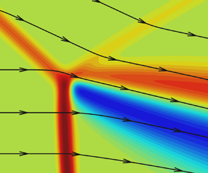
In order to quantify the size of the observed small viscous flow region in comparison to the macroscopic length scales of the flow, the density isolines in the whole computational domain (Block 0) are presented in figure 8(a). First, note that the three-shock solution at the macroscopic level clearly predict the angles of all shocks well. The angle of the slip line of the three-shock solution agrees well with that of the shear layer obtained in the computation, at least up to distances of approximately 10 % of the wedge length from the triple point. The area where the pressure and flow deflection angle are within a 1 % margin from the three-shock solution is shown in green. This is a significant region behind the reflected shock and above the shear layer. Its size, which is approximately 15 % of the wedge length, is nearly independent of the Reynolds number. There is another narrow portion of the flow field on the lower boundary of the shear layer where the parameters are close to the three-shock solution, yet it is much smaller than the upper one. The other part of the flow behind the Mach stem is not predicted by the three-shock solution. The fact that the intrinsically local solution is not valid here can be expected even without taking viscosity into account, because the Mach stem is curved and the flow behind it is subsonic. The high-pressure region behind the shock wave intersection discussed above is shown in red (again a 1 % margin has been chosen). It can be considered a region where the three-shock solution is clearly invalid due to viscosity effects. The region size is at least one order of magnitude smaller than that of the green area, and as will be shown below, is defined mainly by the mean free path length scale and therefore decreases with the Reynolds number. Note that we cannot speak strictly about the size of the regions, because the choice of 1 % margin is rather arbitrary.

Figure 8. (a) Density contours: green area indicates pressure and deflection angle are within 1 % of the three-shock solution; red area indicates pressure is higher than 1 % from the three-shock solution; white area indicates discontinuities in the three-shock solution. (b) Pressure and (c) flow deflection angle, in Block 3, with selected streamlines: green area indicates parameters are within 1 % of the three-shock solution; blue and red areas indicate parameters are lower or higher than 1 % from the three-shock solution.
One can look at this high-pressure region more closely in figure 8(b). The size of this region is approximately 100 mean free paths, and it is located mainly behind the reflected shock, although some part of it is located behind the shear layer. Farther from the shock intersection, the pressure is close to the three-shock solution behind both the Mach stem and the reflected shock, up to distances of approximately 150 mean free paths for the streamline passing through the triple point. A similar field for the deflection angle in figure 8(c) demonstrates that in the vicinity of the shock intersection, the flow deflection angle is lower than that predicted by the three-shock theory except for the streamline passing through the triple point, where it is greater than the three-shock theory value. It can also be demonstrated by comparing the positions of points A, B, C, D and E in the flow fields with their positions on the polar in figure 5(c). Note, on the one hand, that the direction of streamline passing through point C agrees well with the direction of the slip line in the three-shock solution; on the other hand, there is more than 1 % difference in the deflection angle: the flow in the shear layer is deflected more than is predicted by the shock wave solution. It corresponds to the position of point C on the polar. There is a very narrow region on the lower boundary of the shear layer where the flow direction is predicted by the inviscid theory, while this region is much bigger above the shear layer, which is in agreement with figures 8(a,b). Again comparing the positions of the points in the flow fields and on the polar, one can conclude that the non-Rankine–Hugoniot zone is significantly (almost by one order of magnitude) smaller than the equalisation zone where non-Rankine–Hugoniot relations are satisfied but the flow parameter values clearly contradict the three-shock theory. In particular, this is true for the segment DE and even for some part of the reflected shock above.
5.2. Passage to the inviscid limit
The free-stream mean free path  $\lambda _\infty$ is the only independent length scale in the problem of the internal structure of the shock wave. For this reason, naturally, the solution obtained in coordinates normalised to $\lambda _\infty$ does not depend on the Reynolds number. In the irregular reflection of shock waves, there are additional length scales: the wedge length $w$, and the distance from the wedge trailing edge to the symmetry line $g$. In fact, the independent dimensionless parameters are the Reynolds number based on one of the length scales (e.g. $\textit {Re}_w$) and the ratio $g/w$. The following question is natural: does the flow field inside the region of shock wave interaction depend on these parameters? Of primary interest is the dependence on the Reynolds number $\textit {Re}_w$, which can vary within a wide range.
The flow fields near the triple point at  $\textit {Re}_w=10^4$ and $10^{8}$ are compared in figure 9. Here, the coordinates are normalised to the mean free path of molecules in the free stream for the corresponding Reynolds number. The flow fields are shifted so that the shock wave intersection positions match each other. This shift is necessary because the Mach stem heights, and hence the triple point positions, are different at different Reynolds numbers.

Figure 9. Comparison of flow fields near the triple point at two Reynolds numbers: (a) pressure; (b) pressure in the enlarged region; (c) Mach number in the enlarged region; (d) flow deflection angle in the enlarged region.
Figure 9(a) shows the flow field near the triple point with size approximately  ${100\lambda _\infty \times 100\lambda _\infty }$. It is seen clearly that the pressure contours inside the region with size approximately ${30\lambda _\infty \times 30\lambda _\infty }$ coincide completely both inside the shock waves and behind them. Noticeable differences in the pressure contours obtained at different $\textit {Re}_w$ are observed only at a larger distance downstream from the interaction region. The region with size approximately ${30\lambda _\infty \times 30\lambda _\infty }$ is zoomed out in figures 9(b,d). The zone of increasing pressure (figure 9b), which is not described by the inviscid three-shock theory, is observed even at $\textit {Re}_w=10^{8}$. In fact, figure 9(b) shows the vicinity of point C presented in figure 5(b), where a significant difference between the viscous and inviscid solutions is observed. Figures 9(c,d) show the Mach number and deflection angle flow fields, where the shear layer emanating from the shock wave interaction region is visible, in contrast to the pressure field. As is seen, the isolines coincide completely in a small vicinity of the triple point inside the shear layer.
For a more detailed quantitative comparison of flow fields at different Reynolds numbers, figure 10 shows the numerical data in the  $(\theta, p/p_\infty )$ plane along with the shock polars (figure 10a) and the pressure distributions at various $y/\lambda _\infty$ along with the three-shock theory prediction (figure 10b). The pressure and deflection angle distributions along the black dashed curve in figure 9(a) are plotted in figure 10(a). It is seen clearly that the numerical data at all $\textit {Re}_w$ values agree well with each other. As concerns the pressure distributions along the horizontal lines, they also coincide at different $\textit {Re}_w$. In all cases, the pressure behind the shock waves is higher than that in the three-shock solution. Along the line $y/\lambda _\infty =870$ passing through the non-Rankine–Hugoniot zone, the pressure in the region close to point C in figure 10(a) exceeds the inviscid solution by almost 10 %. The results computed at the intermediate Reynolds number $\textit {Re}_w=10^6$ also confirm that the flow pattern around the triple point in coordinates normalised to $\lambda _\infty$ remains unchanged despite the change in the Reynolds number. The contours and the pressure distributions at $\textit {Re}_w=10^6$ are not shown because in the coordinates $(x/\lambda _\infty, y/\lambda _\infty )$, they are not distinguishable from the results presented for other Reynolds numbers.

Figure 10. Comparison of the numerical solutions at different Reynolds numbers: (a) the  $(\theta, p/p_\infty )$ plane; (b) pressure distributions at various $y/\lambda _\infty$.
It should be emphasised that the mean free paths at  $\textit {Re}_w=10^4$ and $10^{8}$ in non-normalised coordinates differ by $10^4$ times. The entire range of the $x$ coordinate over which the pressure distribution at $\textit {Re}_w=10^{8}$ is presented (figure 10b) is smaller than the mean free path at $\textit {Re}_w=10^4$. Nevertheless, being normalised to $\lambda _\infty$, they coincide completely.
Note that the maximum Reynolds number  $10^8$ considered in the present study is somewhat close to the upper limit attainable in ground-based aerodynamic experiments.
5.3. Total enthalpy behaviour in the non-Rankine–Hugoniot zone
For a more detailed study of the non-Rankine–Hugoniot zone, we consider the total enthalpy distribution. According to the Rankine–Hugoniot relations, the total enthalpy is constant across the shock wave in a steady flow of an inviscid and non-heat-conducting fluid. For a viscous heat-conducting fluid, the total enthalpy changes inside the shock wave, but its values ahead of and behind the shock wave are equal (for more details, see e.g. Shoev, Timokhin & Bondar Reference Shoev, Timokhin and Bondar2020).
Figure 11(a) shows the total enthalpy field near the triple point. As shown in the previous subsection, the flow fields near the three-shock intersection in coordinates normalised to the mean free path  $\lambda _{\infty }$ are identical at different Reynolds numbers, so the results reported in this subsection are relevant for a wide range of $\textit {Re}_w$. The total enthalpy increases inside the shock wave, reaches the maximum value, and then decreases; behind the shock wave, the total enthalpy is again equal to its free-stream value. A noticeable exception is the shear layer, where the viscosity effects lead to the non-uniform distribution of the total enthalpy.

Figure 11. Numerical solution at the Prandtl number  $\textit {Pr} = 2/3$: (a) total enthalpy field near the triple point; (b) total enthalpy distributions at various $y/\lambda _\infty$.
The total enthalpy distributions along the lines  $y/\lambda _\infty =850$, $870$ and $890$ are shown in figure 11(b). At $y/\lambda _\infty =890$, one can see perfect recovery of the total enthalpy behind the IS and RS because the line is far from the shock wave intersection. The characteristic peaks inside the IS and RS are separated by a distance much greater than the shock wave thickness. At $y/\lambda _\infty =870$, the total enthalpy behind the incident shock wave does not have enough space to return to its free-stream value; instead, it passes smoothly to the distribution inside the reflected shock wave. In the region of shock wave intersection, the distance along the $x$ axis between the total enthalpy peaks is comparable with the shock wave thickness. The total enthalpy behind the RS is not recovered because of the non-uniform shear layer flow. Further downstream, the line $y/\lambda _\infty =870$ leaves the shear layer because the shear layer is not aligned with the horizontal axis. As a result, the total enthalpy approaches its free-stream value at a distance of approximately $50\lambda _\infty$. At $y/\lambda _\infty =850$, the peak of the total enthalpy inside the MS is significantly higher than peaks inside other shock waves. It is explained by a greater shock strength of the MS. The total enthalpy is recovered behind the MS, then it changes in the shear layer.
According to the Navier–Stokes solution for the viscous shock transition, the total enthalpy is strictly constant everywhere, including the shock transition interior if  ${\textit {Pr} = 3/4}$ (see also Appendix A). This property is used below to better visualise the location of the non-Rankine–Hugoniot zone.
The total enthalpy field computed with  $\textit {Pr} = 3/4$ (all other parameters are the same) is shown in figure 12. The black solid contours (figure 12a) are the pressure isolines $p/p_\infty =1.01$, 9.1, 9.15 and 19.6, which approximately show the boundaries of the shock waves. The total enthalpy inside the shock waves is indeed constant everywhere except for the region of shock wave intersection. It is seen in figure 12(a) that the shear layer is formed inside the region where all shock waves merge together in the vicinity of the point $(x/\lambda _\infty, y/\lambda _\infty ) = (673, 867)$. The flow parameters behind this region cannot be predicted by the Rankine–Hugoniot relations because it is impossible to identify a separate shock wave. The one-dimensional viscous shock transition solution is not applicable in this region either because the flow here is essentially two-dimensional. Therefore, a deviation of the total enthalpy from a constant value could be expected. A noticeable change in the total enthalpy is observed inside the region of shock wave confluence between the pressure contours $p/p_\infty =1.01$ and $19.6$. In fact, it visualises the non-Rankine–Hugoniot zone. It is important to note that in contrast to the inviscid case, the shear layer in the Navier–Stokes computations does not originate from a point; instead, it emerges as a finite-size spot (approximately $10\lambda _\infty$; see figure 12a) immediately behind or even inside the region of shock wave interaction. The distributions at ${y/\lambda _\infty =850}$, $870$ and $890$ are presented in figure 12(b), where the total enthalpy is plotted on the same scale as for $\textit {Pr} = 2/3$. At $y/\lambda _\infty =890$, the total enthalpy is constant with high precision because this line is taken far from the region where the shock waves and the shear layer interact. At $y/\lambda _\infty =870$, the total enthalpy increases inside the reflected shock wave and the shear layer, then it decreases further downstream. Finally, at $y/\lambda _\infty =850$, the total enthalpy increases only slightly inside the Mach stem, while further downstream it first decreases and then increases again in the shear layer. It should be noted that the increase in the Prandtl number from $\textit {Pr} = 2/3$ to $3/4$ reduces the total enthalpy deviation inside the shear layer from the free-stream value. For example, at $y/\lambda _\infty = 850$, the minimum value is $-0.013$ at $\textit {Pr} = 2/3$ (figure 11b) and $-0.009$ at $\textit {Pr} = 3/4$ (figure 12b).

Figure 12. Numerical solution at the Prandtl number  $\textit {Pr} = 3/4$. (a) Total enthalpy field near the triple point. The black solid contours indicate the shock wave boundaries. (b) Total enthalpy distributions at various $y/\lambda _\infty$. (c) Total enthalpy distributions along lines $L_1$, $L_2$ and $L_3$ crossing the shear layer.
The total enthalpy is not equal to its free-stream value inside the shear layer downstream from the non-Rankine–Hugoniot zone. The shear layer thickness grows downstream. The total enthalpy distribution across the shear layer is non-monotonic (figure 12c). It is seen that the shear layer consists of two parts, where the total enthalpy values are lower and higher than its free-stream value, respectively.
Let us consider in more detail the region where the shock waves meet (figure 13). Figures 13(a,c) additionally show the vertical blue lines corresponding to several  $x/\lambda _\infty$ values, and the inclined pink lines $L_{b}$, $L_{c}$, $L_{t}$ along which the total enthalpy distributions are plotted in figures 13(b,d). The total enthalpy is constant along the line ${x/\lambda _\infty =669}$ in figure 13(b) because the shock waves do not yet interact there and are clearly separated from each other. However, slightly (only by $\lambda _\infty$) downstream, the total enthalpy noticeably deviates from the constant value: a small peak appears inside the incident shock wave in the distribution at $x/\lambda _\infty =670$. The minimum and maximum are visible in the next distribution at $x/\lambda _\infty =671$, inside the shock wave confluence. Further downstream ( $x/\lambda _\infty =673$ and $676$), the total enthalpy deviates from its free-stream value more and more noticeably. As was demonstrated in figure 12, these peaks of the total enthalpy persist inside the shear layer far beyond the region of shock wave interaction. It should be noted that there is a local maximum in the total enthalpy field inside the region of shock wave interaction, which is evidenced by the presence of a closed isoline (through which the line $L_{c}$ passes; figure 13c).

Figure 13. Numerical solution at  $\textit {Pr} = 3/4$. (a,c) Total enthalpy field in a small vicinity of the triple point. The black solid contours approximately indicate the shock wave boundaries. (b,d) Total enthalpy distributions along several vertical and inclined lines.
5.4. Curvature of the sonic line inside the Mach stem
Passing through the Mach stem, the supersonic flow is decelerated to a subsonic velocity so that the Mach stem in the inviscid case is also a sonic line. The slope of the Mach stem changes from  $90^\circ$ near the symmetry line to the angle predicted by the three-shock theory at the triple point. In a viscous flow, the Mach stem is a finite-thickness shock transition, whereas the sonic line remains infinitely thin. The sonic line inclination can serve as a convenient quantity to characterise the change in the Mach stem shape from the symmetry line to the triple point.
It was shown above that viscous effects lead to noticeable deviations of the flow parameters behind the Mach stem from the I-polar (point B in figure 10a). Visualisation of the sonic line reveals an important feature of the viscous flow: the sonic line has an inflection close to the triple point (figure 14). Figure 14(a) shows the shape of the sonic line  $x_{son}(y)$; the inflection point is the point where the second derivative vanishes, ${\partial ^2 x_{son}}/{\partial y^2} = 0$. The existence of the inflection point is hardly visible in figure 14(a); however, it is evident from figure 14(b), where ${\partial ^2 x_{son}}/{\partial y^2}$ is plotted. Here, point B is the same as in previous figures. As was shown by Tan, Ren & Wu (Reference Tan, Ren and Wu2006), the existence of the MS inflection near the triple point is more pronounced at other free-stream parameters.

Figure 14. (a) Deflection angle flow field near the triple point. The black solid curve is the sonic line. The streamlines are indicated by arrows. (b) Second derivative  ${\partial ^2 x_{son}}/{\partial y^2}$ versus $y/\lambda _\infty$. (c,d) Fields of the mass flux components $\rho u$ (c) and $\rho v$ (d).
The fields of the mass flux components  $\rho u$ and $\rho v$ (figures 14c,d) reveal two regions with closed contours of $\rho u$ separated by a line passing through the inflection point. At the same time, a closed isoline of $\rho v$ in figure 14(d) is located well above the inflection point and corresponds to the closed contour in the field of the flow deflection angle seen in figure 9(d). The inflection point on the MS observed in the Euler computations of Tan et al. (Reference Tan, Ren and Wu2006) was connected, most probably, with not physical but numerical viscosity, which is an inherent feature of shock-capturing schemes. Generally speaking, the form of the numerical viscosity differs from the viscous terms of the Navier–Stokes equations; nevertheless, the numerical viscosity still works in such a way that shock waves acquire an internal structure. Therefore, it can be assumed that the mechanisms of the emergence of the inflection point in these two cases are similar, and its existence is a specific feature of the irregular interaction of finite-thickness shock waves. This assumption can be verified by solving the Euler equations with a shock-fitting scheme, as was done e.g. by Ivanov et al. (Reference Ivanov, Bonfiglioli, Paciorri and Sabetta2010b) and Ivanov, Paciorri & Bonfiglioli (Reference Ivanov, Paciorri and Bonfiglioli2010c) for other flow conditions.
6. Numerical results: the weak reflection
6.1. Effects of viscosity and passage to the inviscid limit
As was noted above, a numerical study of the weak reflection in a steady viscous flow was undertaken earlier by Ivanov et al. (Reference Ivanov, Shoev, Khotyanovsky, Bondar and Kudryavtsev2012), and the passage to the inviscid limit was investigated. In that paper, however, only the case where the three-shock solution does not exist (the von Neumann paradox conditions) was considered. In the present paper, we have performed similar computations for a more common situation when the I- and R-polars intersect, and the three-shock solution exists. The essential difference between the considered strong and weak reflections is that the flow behind the RS is subsonic in the latter case.
The computations are performed at the following values of the flow parameters:  $M_\infty = 1.7$, $\gamma = 5 / 3$, $\theta _w = 8.5^\circ$, and various $\textit {Re}_w$. The shock polars for $\theta _w = 8.5^\circ$ are shown in figure 2(b); the three-shock solution corresponds to point B(C).
The pressure fields near the triple point at various Reynolds numbers (from  ${\textit {Re}_w=4\times 10^3}$ to $\textit {Re}_w=2\times 10^8$) are shown in figure 15. The black solid lines show the locations of the shock waves and the slip line predicted by the three-shock theory. It is seen that the slopes of RS and MS at $\textit {Re}_w=4\times 10^3$ do not agree well with the inviscid solution. As the Reynolds number is increased, the agreement between the numerical solution and the three-shock theory becomes better and better. Despite a significant change in the shock wave slopes with an increase in the Reynolds number, there are only minor changes ( ${\sim }0.5\,\%$) in pressure behind these shock waves.

Figure 15. Pressure fields near the triple point at  $M_\infty =1.7$, $\gamma =5/3$, $\theta _w=8.5^\circ$: (a) $\textit {Re}_w=4 \times 10^3$; (b) $\textit {Re}_w=4 \times 10^4$; (c) $\textit {Re}_w=8 \times 10^6$; (d) $\textit {Re}_w=2 \times 10^8$. The black solid lines show the shock wave locations predicted by the three-shock solution.
The fields of the flow deflection angle computed at  $\textit {Re}_w=4 \times 10^3$ and $2 \times 10^8$ are shown in figures 16(a,b). As is seen clearly, in contrast to pressure, the flow deflection angle changes significantly: the maximum value increases from approximately $4.2^\circ$ to approximately $6.484^\circ$. At higher Reynolds numbers, the shear layer is thinner, and its slope tends to the slip line angle predicted by the three-shock theory. For a more detailed analysis of the flow near the triple point, we plot in figure 16(c) the flow deflection angle distributions along lines $L1$,
$L1$,  $L2$,
$L2$,  $L3$ (figure 16(a), $\textit {Re}_w=4\times 10^3$) and $L1$*, $L2$*, $L3$* (figure 16(b), $\textit {Re}_w=2\times 10^8$). The distributions at low and high Reynolds numbers are shown by solid curves and symbols, respectively.

Figure 16. Numerical solutions of the Navier–Stokes equations at different Reynolds numbers. Flow deflection angle field at (a)  $\textit {Re}_w=4 \times 10^3$, and (b) $2 \times 10^8$. The black solid curves show the shock wave locations predicted by the three-shock theory. (c) Distributions of the flow deflection angle along several horizontal lines. The slope of the slip line predicted by the three-shock solution is shown as SL. (d) Numerical data plotted in the $(\theta, p/p_\infty )$ plane along with the shock polars.
Lines  $L1$ and $L1$* pass through the IS and RS. It is seen clearly that inside the IS (this region is indicated as the ‘IS profile’) the distributions along $L1$ and $L1$* completely coincide when plotted in the $x/\lambda _\infty$ coordinates. As for the RS, the distributions inside it at different $\textit {Re}_w$ coincide up to a certain point. After that, the distributions diverge so that the flow deflection angle behind the RS is noticeably smaller at the lower Reynolds number. The curvature of the RS in the normalised coordinates is larger at low $\textit {Re}_w$. As a result, the slope of the RS at the intersection with $L1$ is noticeably different from that predicted by the three-shock solution. This difference is much smaller at higher $\textit {Re}_w$ since the RS shape is closer to the straight line.
Lines  $L2$ and $L2$* pass through the region of shock wave confluence. The distributions along $L2$ and $L2$* already differ inside the IS. More exactly, the profiles also coincide up to a certain point and diverge rapidly behind it. At high Reynolds numbers, the distribution along $L2$* has a small peak, which almost reaches the theoretical value at the triple point labelled as SL in figure 16(c).
A similar behaviour is also observed for the distributions along lines  $L3$ and $L3$* passing through the MS. At first, they almost coincide inside the MS; however, farther downstream they diverge significantly. As earlier, this is explained by a larger curvature of the MS (in the normalised coordinates) at low $\textit {Re}_w$.
It should be noted that the flow deflection angle at high Reynolds number is nearly the same in the whole region behind the shock waves. It is somewhat lower than SL value, the theoretical value at the triple point. A different behaviour is observed at low Reynolds number: behind the shock waves, the distributions along the lines  $L1$ and $L2$ are fairly close to each other, whereas the distribution along $L3$ behind the MS is noticeably different from them.
The results computed at five different Reynolds numbers are compared in figure 16(d) in the  $(\theta, p/p_\infty )$ plane. It is seen clearly that an increase in the Reynolds number leads to an increase in the maximum flow deflection angle, whereas the pressure remains nearly the same, which was actually demonstrated above in considering the isobars near the triple point. At $\textit {Re}_w = 2 \times 10^8$, the numerical data approach closely the shock polar intersection, which represents the three-shock solution. It can be expected that the inviscid solution will be reached in the limit $\textit {Re}_w \to \infty$. This behaviour is qualitatively consistent with that obtained previously in studying the weak reflection shock waves under the von Neumann paradox conditions. In both cases, the viscous solution tends to the inviscid configuration as the Reynolds number increases, with only one difference: this is a configuration corresponding to the four-wave solution in the case of the von Neumann paradox and a simpler, three-shock, configuration in the present case. On the other hand, the numerical simulations also show that the viscosity plays an important role in the formation of the flow structure near the triple point in a wide range of Reynolds numbers, and significantly changes the mechanism of interaction of three intersecting shock waves.
Figure 17 shows the density near the triple point at  $Re_w = 2\times 10^8$ and five density distributions at various Reynolds numbers along lines $L_{t}$, $L_{c}$ and $L_{b}$. The lines are parallel to the slip line of the three-shock solution and chosen so that $L_{t}$ passes across the IS and RS, $L_{c}$ passes through the shock interaction region entering the shear layer, and $L_{b}$ passes across the MS. The $L_{c}$ line passes through the origin (the triple point of the three-shock solution), while $L_{t}$ and $L_{b}$ intercept the $y$ axis 40 mean free paths above and below the origin, respectively. The distributions along $L_{t}$ show that the density behind the RS tends to the three-shock solution as the Reynolds number increases. The deviation from the three-shock solution decreases with $Re_w$; in particular, it is less than 0.2 % at $Re_w > 8\times 10^5$. The density distributions along $L_{c}$ show that in the plotted region inside the shear layer, the numerical viscous solution at $Re_w > 8\times 10^5$ predicts almost a constant density value between the values predicted by the three-shock solution behind the RS and MS. At $Re_w < 8\times 10^5$, the density does not reach a plateau and decreases downstream from the triple point. In an inviscid flow, the density has a jump across the slip line likewise in a shock wave, therefore in a viscous flow, the density inside the shear layer has a value somewhere in between the values across the slip line. It is necessary to note that the pressure and deflection angle have no jumps across the slip line in an inviscid flow. That is why the numerical data in the $(\theta, p/p_\infty )$ plane tend to the shock polar intersection point (inviscid three-shock solution) as the Reynolds number grows. The density distribution along $L_{b}$ also shows convergence of the numerical viscous solution to the inviscid three-shock solution with an increase in the Reynolds number. More exactly, the deviation of density behind the MS is smaller than 0.4 % at $Re_w > 8\times 10^5$.

Figure 17. Density contours and distributions at various  $Re_w$. (a) Density contours at $Re_w = 2\times 10^8$. The black solid lines show the three-shock solution. Lines $L_{t}$, $L_{c}$ and $L_{b}$ are parallel to the slip line of the three-shock solution. (b–d) Density distributions at various $Re_w$ along lines (b) $L_{t}$, (c) $L_{c}$, and (d) $L_{b}$. Lines labelled ‘Three-shock solution RS’, ‘RS’ and ‘Three-shock solution MS’, ‘MS’ show the density according to the three-shock solution behind the RS and MS, respectively. The dashed curves, showing the deviation from the three-shock solution, are labelled ‘Deviation’.
7. Discussion
The results of the numerical simulations of the irregular reflection show that the viscous effects remain substantial near the triple point even at very high Reynolds numbers. In both cases of the strong and weak reflections, there is a non-Rankine–Hugoniot zone downstream of the intersection of the incident shock wave, the reflected shock wave, and the Mach stem. The flow inside the non-Rankine–Hugoniot zone is essentially two-dimensional, and the flow parameters inside it cannot be calculated from the Rankine–Hugoniot relations. The performed numerical simulations show that the solutions of the Navier–Stokes equations in this region behave differently in the limit  $\textit {Re}_w \to \infty$ for strong and weak shock waves.
In the strong reflection, all the shock wave slopes near the triple point are well predicted by the three-shock theory and remain unchanged as the Reynolds number increases. Moreover, there is a substantial region of the supersonic flow behind the reflected shock, where the parameters are very close to those predicted by the three-shock theory. The size of this region is determined by the macroscopic flow structure and equals a fraction of the wedge length (approximately 15 %). On the other hand, for any sufficiently large Reynolds number, there exists a much smaller flow region behind the shock wave intersection (equalisation zone) where certain differences from the inviscid three-shock solution are observed; in particular, the pressure there is substantially higher than at the inviscid triple point. In an even smaller part of this region (non-Rankine–Hugoniot zone), the parameters behind the reflected shock and Mach stem are not predicted by the Rankine–Hugoniot relations. The size of this zone is inversely proportional to the Reynolds number and is of the order of magnitude of dozens of mean free paths. The structure of the non-Rankine–Hugoniot zone is similar for various Reynolds numbers. In coordinates normalised with the free-stream mean free path, the numerical solution inside the zone does not depend on the Reynolds number. The numerical data presented in the  $(\theta, p/p_\infty )$ plane are identical at all examined values of the Reynolds number and do not approach the shock polar intersection even as $\textit {Re}_w$ increases. This means that the numerical solution of the Navier–Stokes equations in this region is always different from the three-shock solution, even as $\textit {Re}_w \to \infty$. This deviation is fairly noticeable, e.g. the difference in pressure is approximately 10 % for the considered flow parameters. Thus the assumption of Sternberg (Reference Sternberg1959) that the viscous solution does not tend to the inviscid one as $\mu \to 0$ in the strong reflection can be considered as valid. More exactly, the pointwise convergence takes place in physical coordinates; however, the uniform convergence is not observed. In the mean free path coordinates, outside the shock waves downstream from the triple point, the solution does not depend on $Re_w$ and is different from the inviscid one, so there is neither uniform nor pointwise convergence to the inviscid solution.
At the same time, in the weak reflection, a different scenario of the transition to the inviscid limit is observed. Even at the examined (quite high) Reynolds numbers, the flow fields near the triple point are not similar and do not coincide in the coordinates normalised to the internal viscous scale, such as e.g. the mean free path of molecules. As the Reynolds number increases, the numerical data presented in the  $(\theta, p/p_\infty )$ plane get closer and closer to the inviscid solution being the shock polar intersection in the case discussed here. It is valid both at the von Neumann paradox conditions (Ivanov et al. Reference Ivanov, Shoev, Khotyanovsky, Bondar and Kudryavtsev2012) and in a more typical case considered in the present paper when the three-shock solution exists. At relatively low Reynolds numbers, the shock wave slopes near the triple point are clearly different from those predicted by the three-shock theory, but converge to the inviscid theoretical prediction with increasing Reynolds number. One cannot say that the flow fields converge uniformly to the solution of the Euler equations because the shock waves always have a finite thickness at any finite Reynolds number. The magnitude of this difference is of the order of the jump of gas-dynamic variables across the shock wave. Nevertheless, the flow parameters near the triple point outside the shock waves approach the inviscid three-shock theory predictions as the Reynolds number increases. One should, however, keep in mind that the numerical solution approaches the three-shock theory values only in the near vicinity of the shock intersection; the parameters behind both the Mach stem and reflected shock are not constant, and a macroscopic flow region with parameters predicted by the three-shock theory typical of the strong reflection is not observed. In fact, there is not a single point in the flow behind the shocks where the deflection angle reaches exactly or exceeds the three-shock theory value even at the highest Reynolds number modelled.
Apparently, the different behaviour of the solutions of the Navier–Stokes equations in the strong and weak reflections is caused by the differences in the mechanisms of shock wave interaction in these two cases. As has been mentioned already, from the physical perspective, the most substantial difference between these two cases is that the flow behind the reflected shock is supersonic for the strong reflection, while it is subsonic for the weak reflection.
In the strong reflection, the flow in the shock wave interaction region is governed by two factors: inviscid shock wave interaction effects described by the three-shock theory (with no characteristic length scale), and viscous effects with the length scale proportional to the mean free path. It leads to the local viscous solution, which is independent of the macroscopic length scale of the wedge size (hence independent of the Reynolds number).
In the weak reflection with the subsonic flow behind the reflected shock wave, the shock wave interaction region can be significantly affected additionally by the downstream flow, which depends on the macroscopic geometric parameters of the problem: the finite size of the wedge and the ratio  $g/w$. This third factor leads to the dependence of the local viscous solution in the shock interaction region on two different length scales: mean free path and wedge size. This is why the local interaction region solution clearly depends on the Reynolds number, which is proportional to the ratio of the wedge size and mean free path. In contrast to the strong reflection, the reflected shock wave is curved, and the length scale of the wedge size governs its curvature. When the mean free path coordinates are used, the curvature radius is proportional to the Reynolds number. Only for the highest Reynolds numbers considered in the present work are the reflected shock and Mach stem curvatures negligible in the vicinity of the interaction region on the length scales of 100 free-stream mean free paths. For lower Reynolds numbers, the curvature is so substantial that its radius is commensurable with the shock thickness, and there is a clear deviation from the three-shock theory in terms of the slopes of the reflected shock and the Mach stem. With an increase of the Reynolds number, the shock wave angles and the numerical data in the $(\theta, p/p_\infty )$ plane converge to those predicted by the three-shock theory.
The above reasoning explains in part the difference between the behaviour of the viscous solution for the strong and weak reflections in the limit  $\textit {Re}_w \to \infty$. However, it is not clear why the uniform convergence to the inviscid solution seems to take place for the weak reflection while this is not the case for the strong reflection. The case of the highest considered Reynolds number of the weak reflection is similar to the strong reflection due to the fact that all three shock waves in the vicinity of the interaction region are straight and their slopes coincide with the three-shock solution. However, as can be inferred from the $(\theta, p/p_\infty )$ results, the viscous solution for the weak reflection converges to the three-shock theory values, while in the strong reflection one observes a clear deviation from the inviscid solution (non-Rankine–Hugoniot zone). Probably, this difference can be explained by much sharper gradients in the strong reflection. In particular, as can be seen in figure 2(a), the R-polar has a very steep slope near point B(C), so a small deflection of the flow behind the reflected shock wave leads to a significant change of pressure, while for the weak reflection (see figure 2b), we cannot expect a significant change of pressure. A non-Rankine–Hugoniot zone, somewhat similar to that observed in the strong reflection, can possibly persist in the weak reflection even in the limit $\textit {Re}_w \to \infty$, while just being not recognisable in the $(\theta, p/p_\infty )$ or flow field data due to really minute deviation from the inviscid solution.
One of the possible limitations of the present study is that the flow analysis is based on the Navier–Stokes equations, while the zone of interest is several dozens of mean free paths in size and local gradients are quite high, especially in the strong reflection, so non-equilibrium effects are possible. However, one can conclude from previous works (Khotyanovsky et al. Reference Khotyanovsky, Bondar, Kudryavtsev, Shoev and Ivanov2009; Ivanov et al. Reference Ivanov, Bondar, Khotyanovsky, Kudryavtsev and Shoev2010a) that major qualitative differences between the Navier–Stokes and the DSMC (or the Boltzmann equation) solutions can hardly be expected in the studied flow region. Another point is that the present work can be considered a study of the Navier–Stokes solution convergence behaviour as  $Re \to \infty$, which would make sense from the mathematical perspective even if the equations did not capture the flow phenomena accurately.
8. Conclusions
The influence of viscosity on the flow structure near the triple point in the strong ( $M_\infty =4$) and weak ( $M_\infty =1.7$) irregular reflection of shock waves has been studied by solving numerically the Navier–Stokes equations. It has been found that in both cases, the so-called ‘non-Rankine–Hugoniot zone’ emerges due to the interaction of viscous, finite-thickness shock transitions. The flow in this zone is essentially two-dimensional, so the flow parameters behind this zone cannot be determined from the Rankine–Hugoniot relations.
The numerical solutions of the Navier–Stokes equations in the strong and weak reflection of shock waves behave significantly differently as the Reynolds number increases.
At  $M_\infty =4$, the flow fields near the triple point at different Reynolds numbers are self-similar and coincide in the coordinates normalised to $\lambda _\infty$, the mean free path of molecules in the free stream. The flow parameters behind the reflected wave and the Mach stem differ from those predicted by the inviscid three-shock theory. More exactly, as $\textit {Re} \to \infty$, the maximum difference between the inviscid and viscous solutions tends to a non-zero constant value. Thus the convergence of the Navier–Stokes solutions to the solution of the Euler equations as $\textit {Re} \to \infty$ is not uniform. In other words, there is a finite difference between the Navier–Stokes and Euler solutions inside a flow region behind the shock intersection; the size of this region decreases in the physical coordinates as $\textit {Re} \to \infty$, although it remains constant in the coordinates normalised to $\lambda _\infty$.
At  $M_\infty = 1.7$, the flow structure – in particular, the slopes of shock waves – in the vicinity of the triple point depends on the Reynolds number even in coordinates normalised to $\lambda _\infty$. The flow parameters behind the reflected shock wave and the Mach stem approach those predicted by the inviscid theory as $\textit {Re} \to \infty$ due to adjusting of shock wave slopes. Thus in the inviscid limit, the magnitude of the difference between the viscous and inviscid solutions vanishes, along with the size of the region where this difference is observed.
It can be concluded that there is a substantial distinction in the limit behaviour of the Navier–Stokes solutions in the strong and weak reflections of shock waves. Presumably, this distinction is due to the subsonic flow behind the reflected shock wave, and much weaker gradients in the near vicinity of the shock interaction region in the weak reflection.
Acknowledgements
This paper is dedicated to the bright memory of Professor M. Ivanov, who was a tireless researcher of shock wave interactions and initiated our interest in viscous effects in the irregular reflection. We would also like to acknowledge the role of Professor J. Sternberg, who pioneered the investigation of this subject and kindly discussed some aspects of the problem with the authors.
Funding
The second and third authors (A.N.K. and D.V.K.) acknowledge the support of the Russian Science Foundation under grant no. 18-11-00246- $\Pi$. The work of the first and fourth authors (G.V.S. and Ye.A.B.) was supported by the Russian Science Foundation under grant no. 22-19-00750. The computations were performed at the Supercomputer Centre of Novosibirsk State University (nusc.nsu.ru).
Declaration of interests
The authors report no conflict of interest.
Appendix A
Let us consider a fluid flow intersecting a steady oblique shock wave. As everywhere in the paper, the fluid is assumed to be a perfect gas with the shear viscosity and heat conductivity depending on the temperature, and the bulk viscosity equal to zero. The coordinate normal to the wave front is  $x$, the coordinate along the wave is $y$, the corresponding velocity components are $u$ and $v$, and the density, pressure, temperature and viscosity are $\rho$, $p$,
$p$,  $T$ and $\mu$, respectively. The constant values of flow parameters ahead of and far behind the shock wave are marked by the subscripts 1 and 2, respectively.
If the shock wave slope is constant and therefore the derivatives of all variables with respect to  $y$ are equal to zero, then the Navier–Stokes equations can be written as follows:
 $$\begin{gather} \frac{{\rm d}}{{\rm d} x} (\rho u ) = 0, \end{gather}$$
 $$\begin{gather}\frac{{\rm d}}{{\rm d} x} (\rho u^2 + p) = \frac{{\rm d}}{{\rm d} x} \left(\frac{4}{3}\,\mu\,\frac{{\rm d}u}{{\rm d} x}\right), \end{gather}$$
 $$\begin{gather}\frac{{\rm d}}{{\rm d} x} (\rho uv ) = \frac{{\rm d}}{{\rm d} x} \left(\mu\,\frac{{\rm d}v}{{\rm d}x}\right), \end{gather}$$
 $$\begin{gather}\frac{{\rm d}}{{\rm d}x} (\rho u H) = \frac{{\rm d}}{{\rm d}x} \left(\frac{\mu c_p}{\textit{Pr}}\,\frac{{\rm d}T}{{\rm d} x}\right) + \frac{{\rm d}}{{\rm d}x}\left(\frac{4}{3}\,\mu u\,\frac{{\rm d}u}{{\rm d}x} \right). \end{gather}$$
Here,  $H=c_pT + {(u^2+v^2)}/{2}$ is the total enthalpy.
These equations can be integrated once:
 $$\begin{gather} m \equiv {\rm const} = \rho u = \rho_1 u_1 = \rho_2 u_2, \end{gather}$$
 $$\begin{gather}\frac{4}{3}\,\mu\,\frac{{\rm d}u}{{\rm d} x} = m(u-u_1)+p-p_1, \end{gather}$$
 $$\begin{gather}\mu\,\frac{{\rm d}v}{{\rm d} x} = m(v-v_1), \end{gather}$$
 $$\begin{gather}\frac{\mu c_p}{\textit{Pr}}\,\frac{{\rm d}T}{{\rm d} x} + \frac{4}{3}\,\mu\,\frac{{\rm d}}{{\rm d}x} \frac{u^2}{2} = m (H-H_1). \end{gather}$$
As  $x \to \pm \infty$, the derivatives on the right-hand sides of (A2)–(A4) vanish, which yields the Rankine–Hugoniot relations between the flow parameters with the subscripts 1 and 2; in particular, it follows from (A1), (A2) and (A4) that $v_1=v_2$ and $H_1=H_2$. Then the solution of (A7) is $v=v_1=v_2=\textrm {const}$, i.e. the velocity component tangent to the shock wave is constant everywhere inside the viscous shock transition.
At  $\textit {Pr} = 3/4$, (A8) is reduced to
 \begin{equation} \frac{4}{3}\,\mu\,\frac{{\rm d}H}{{\rm d}x} = m(H-H_1), \end{equation}
whence it follows that in this case, the total enthalpy  $H$ is constant inside the shock wave transition and equal to its free-stream value.


