


Introduction
Ice-shelf shear margins are zones of focused strain localization resulting from steep velocity gradients where relatively fast-flowing ice moves past bedrock or neighboring slower moving ice. They are typically located along the lateral margins of glaciers or within the confluence of glacial streams in ice shelves. Shear zone stability represents a potentially critical control on the mass balance of ice sheets because ice shelves buttress the flow of ice from the ice-sheet interior (Reese and others, Reference Reese, Gudmundsson, Levermann and Winkelmann2018). Observations across Antarctica point to a common sequence of lateral shear zone destabilization that follows initial submarine melt-driven thinning: thinning increases susceptibility to fracture and crevassing, which reduces the load-bearing surface area and lateral drag provided by the ice shelves, and ultimately results in a substantial loss of buttressing potential at the grounding line (Dupont and Alley, Reference Dupont and Alley2005; MacGregor and others, Reference MacGregor, Catania, Markowski and Andrews2012; Khazendar and others, Reference Khazendar, Borstad, Scheuchl, Rignot and Seroussi2015). While several modeling studies have highlighted the crucial role lateral margins play in ice-shelf stability (Khazendar and others, Reference Khazendar, Borstad, Scheuchl, Rignot and Seroussi2015; Favier and others, Reference Favier, Pattyn, Berger and Drews2016), feedbacks between thinning, mechanical weakening and fracture, and calving have only recently been successfully incorporated into numerical ice-shelf modeling (Borstad and others, Reference Borstad2012, Reference Borstad2016). Here we present a statistical approach to predict crevasse initiation in a shear zone based on surface velocity observations and using ground-penetrating radar (GPR) as calibration.
The strong lateral gradients in velocity produce regions of local expansion and tensile failure generates extensive swaths of concentrated crevassing. Multiple studies have laid the groundwork for deriving critical strain rate and principal stress thresholds for crevasse initiation based on field observations (Meier, Reference Meier1958; Kehle, Reference Kehle1964; Vaughan, Reference Vaughan1993). However, crevasse initiation depends on several factors including ice temperature, density, impurities, crystallography and history (Vaughan, Reference Vaughan1993), such that critical thresholds will vary in type and value across different glacial environments. A more thorough understanding of crevasse initiation thresholds could better capture the aforementioned feedbacks between acceleration, crevassing and weakening in large-scale numerical models which currently only parameterize these feedbacks through damage – a scalar variable that quantifies the loss of load-bearing surface area due to ice-shelf fracture. Alternatively, Emetc and others (Reference Emetc, Tregoning, Morlighem, Borstad and Sambridge2018) used a statistics-based approach to predict the location of observed surface fractures based on several potential parameters including flow regime, geometry and mechanical properties of ice. They found the most reliable predictor parameters for modeling surface fractures on ice shelves to be the effective strain rate (i.e. the second invariant of the strain rate tensor) and principal stress.
Understanding crevasse initiation may best be achieved with small-scale observations in which crevasses can be directly observed. While large-scale observations of intensified fracture and rifting have been observed through remote-sensing observations (Borstad and others, Reference Borstad, McGrath and Pope2017), snow cover may obscure the full extent of a crevasse field – particularly in regions of high snow accumulation – requiring in situ observations to accurately map crevasses. We combine crevasse observations from high-frequency GPR surveys and kinematic outputs derived from remotely-sensed ice surface velocities of the McMurdo Shear Zone, Antarctica, to develop a statistical method to investigate the kinematic drivers of crevasse initiation and to estimate crevasse initiation threshold values. While our crevasse initiation strain rate threshold for the McMurdo Shear Zone (MSZ) is not directly transferable to other glacial settings, our method can be used as a tool for monitoring dynamic changes in shear zones through time with minimal in situ data. The method can also be leveraged to optimize safety when collecting in situ observations within or traversing potentially crevassed regions.
The McMurdo Shear Zone
Our study focuses on the MSZ, a relatively well-studied segment of the western lateral margin of the Ross Ice Shelf (RIS) where fast ice (~450 m a−1, estimated from GPS observations during field data acquisition) shears past the slower-moving McMurdo Ice Shelf (MIS; ~200 m a−1), creating a 5–10 km wide zone of intense crevassing (Fig. 1). A weakening of this lateral margin has the potential to destabilize the RIS, as has been observed and modeled on smaller ice shelves (Vieli and others, Reference Vieli, Payne, Shepherd and Du2007; MacGregor and others, Reference MacGregor, Catania, Markowski and Andrews2012; McGrath and others, Reference McGrath2012). Widths of crevasses from ground-truth data in this region have ranged from small <0.5 m-wide cracks to ~14 m-wide (Courville, Reference Courville2015). Near-surface crevasses typically oriented at ~45° to flow (Arcone and others, Reference Arcone2016) indicate relatively recent formation given the rotation associated with shear.
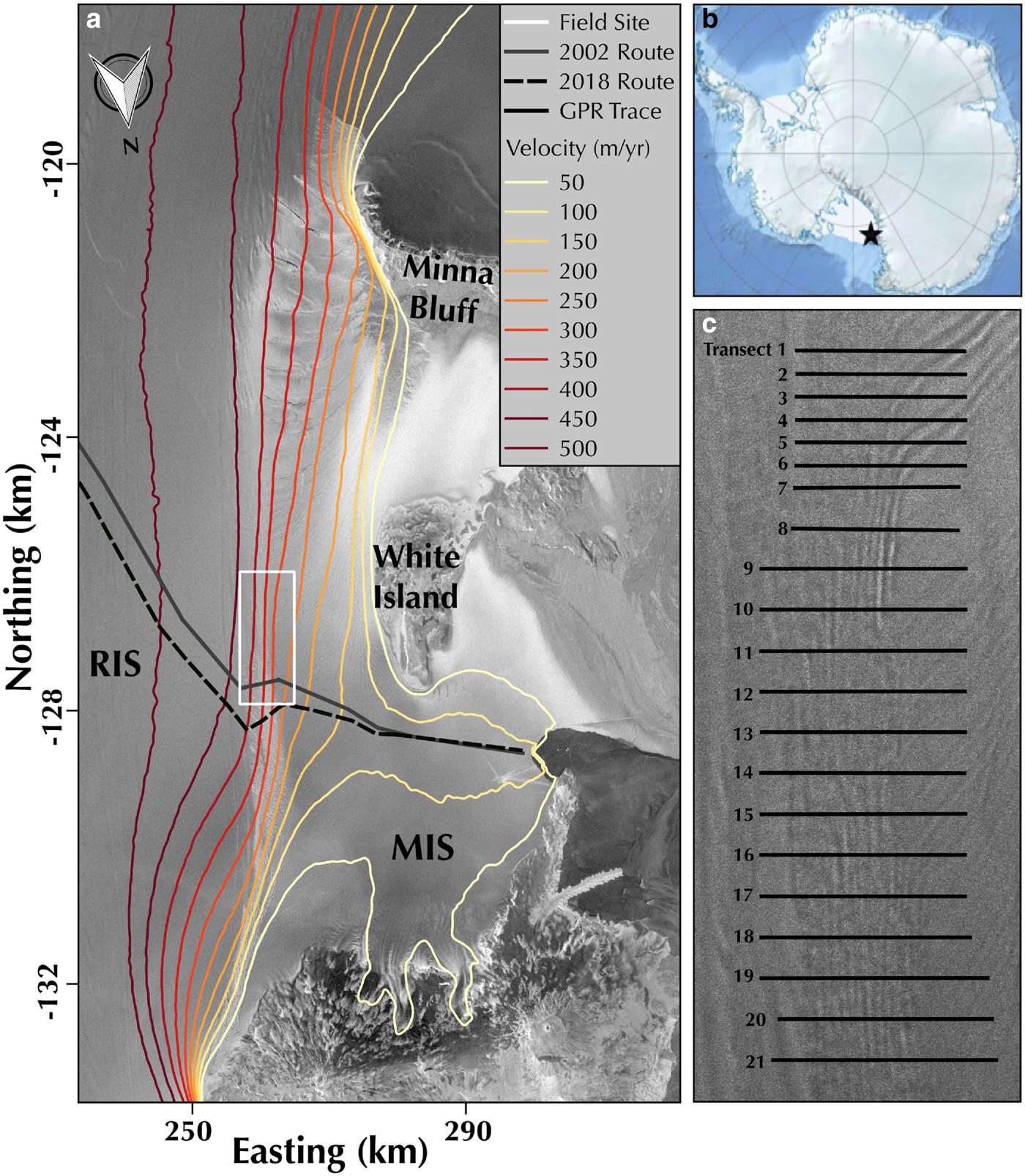
Fig. 1. (a) Radarsat2 image of the MSZ and surrounding area with contour map of ice surface velocity from MEaSUREs2. Location of field study area is outlined in white. Original location of the SPoT traverse in 2002 (determined from GPS waypoints) is noted by the solid dark gray line. The SPoT 2018 route location was derived from Sentinel2 imagery and is noted by the dashed line. The route has advected to the north by ~4 km on its western corner and ~6 km on its eastern corner and has rotated counter clockwise by ~40°. (b) Overview of Antarctica with the location of MSZ noted by black star. (c) Close-up of field area outline in white in the overview panel with GPR transects superimposed on TerraSAR-X image from 2017.
Synchronous and aligned crevassing occurs in the marine ice at ~160 m depth in our study area, despite a lack of evidence of open meteoric englacial fractures (Arcone and others, Reference Arcone2016). This suggests that the englacial ice is under great stress, likely fractured and the greatest source of potential instability. Recent modeling by Reese and others (Reference Reese, Gudmundsson, Levermann and Winkelmann2018) predicts that moderate thinning in this region could have far-reaching effects, including an immediate acceleration of the Bindschadler and MacAyeal ice streams located more than 900 km away. Recent observed changes of summer ice flow direction along the MIS following a break-up event in March 2016 (Banwell and others, Reference Banwell2017; MacAyeal, personal communication; MacDonald and others, Reference MacDonaldin press) suggest that dynamic changes may already be underway in this previously stable region.
The MSZ region is also logistically important to the US and New Zealand Antarctic research programs. The United States Antarctic Program (USAP) annually mitigates crevasse hazards along the South Pole Traverse (SPoT) route that crosses the MSZ. Since the route's creation in 2002 it has advected northward past White Island into a region of greater flow divergence and intensified crevassing motivating the need to chart a new route across the MSZ where crevassing is minimal. Crevasses along the route have been monitored yearly with GPR for infrequent mitigation (filling). Our observations from 2017 add to this dataset and provide the most spatially extensive and robust dataset of in situ crevasse observations to date.
Methods
We analyzed ~95 km of high-frequency GPR data collected within the MSZ in October of 2017. We identified individual crevasse features and estimated their maximum width and overlying snowbridge thickness. Kinematic outputs such as shear strain rate, dilatation rate and vorticity rate were derived from MEaSUREs2 and auto-RIFT ice flow velocities. We estimated the relative frequency distribution of crevasses with respect to the kinematic data outputs. By utilizing these relative frequency distribution plots, we then predicted the number of crevasses along two potential routes across the MSZ. Details of the methods used to process and analyze these data are provided below.
GPR collection and processing
We used a GSSI SIR30 control unit and model 5103 400 MHz antenna unit to record 20 traces s−1 over a time range of 200 ns (~20 m in firn) and 4096 32-bit samples/trace with a time-variable gain. This time range was guided by GPR observations from previous field seasons where minimal crevassing was found below 20 m (Arcone and others, Reference Arcone2016). We deployed two four-wheel-drive battery-powered rovers (Yeti, Trautmann and others, Reference Trautmann, Ray and Lever2009; and Scotty, Lever and others, Reference Lever2013, a later adaptation of Yeti's design) to tow two separate GPR systems (to cover more ground) at a constant speed of ~1.5 m s−1. Each rover was coupled with a Garmin-19x GPS system and followed waypoints along 21 preplanned transect routes orthogonal to overall ice flow direction (Fig. 1). This field survey was designed both to investigate the spatial distribution of crevassing upstream of the SPoT where few observations have been gathered in the past, and to examine the inheritance of past rifting at the tip of Minna Bluff. Transect length and spacing were constrained by rover battery power capabilities and amount of time spent in the field.
We manually identified the leading edge of the direct-coupling wave (i.e. a combination of direct transmission between transmitter and receiver antennas, and a surface reflection) in the radar profiles, and set the depth to zero at that point. We then used the travel time to depth conversion to transform the round-trip transit time into thickness using the following formula

where εr is the dielectric permittivity (dimensionless), c is the speed of light in a vacuum (3 × 10⁸ m s−1) and t is the round-trip transit time (in seconds). A permittivity value of εr = 2.2 was used for a depth of 20 m, as derived from hyperbolic diffractions (Arcone and Delaney, Reference Arcone and Delaney2000; Arcone and others, Reference Arcone2016). This value corresponds to an effective average density of 0.58 kg m−3 (Kovacs and others, Reference Kovacs, Gow and Cragin1982). To reduce data volume and increase the signal-to-noise ratio, we stacked the radar data by averaging adjacent traces together in sets of three. Spatial accuracy before stacking was ~0.2 m per trace with a maximum error of ~0.4 m after stacking. A broadband finite-impulse response filter was applied to the stacked transects to alleviate high-frequency noise and low-frequency modulation (Arcone and others, Reference Arcone2016; Campbell and others, Reference Campbell, Courville, Sinclair and Wilner2017).
Velocity datasets
Kinematic outputs were derived from multiple velocity datasets including MEaSUREs2 and JPL auto-RIFT (Rignot and others, Reference Rignot, Mouginot and Scheuchl2017; Gardner and others, Reference Gardner2018). The MEaSUREs2 velocities were derived using speckle tracking and interferometric phase analysis using RADARSAT-1, RADARSAT-2, ERS-1,ERS-2 and Sentinel-1 SAR platforms, and ENVISAT ASAR acquired from 1996–1997, 2000 and 2007–2016 (Rignot and others, Reference Rignot, Mouginot and Scheuchl2017). In addition, JPL auto-RIFT velocities were derived using feature-tracking techniques from Landsat 7 and Landsat 8 scenes acquired during periods of solar illumination (September–March) from 2013 to 2018 and have a temporal resolution of less than 48 days (Gardner and others, Reference Gardner2018). The MEaSUREs2 dataset was mosaicked as outlined by Rignot and others (Reference Rignot, Mouginot and Scheuchl2011) to produce a 450 m-resolution velocity map with uncertainties of ~3 m a−1 in both x and y directions. The auto-RIFT dataset provided by Gardner and others (Reference Gardner2018) produced yearly velocity maps from 2014 to 2017 at 250 m resolution with uncertainties of 20–30 m a−1 for individual velocity estimates. Both datasets were produced in the Antarctic Polar Stereographic projection (EPSG 3031) with true scale at 71° S. Temporal variations of the auto-RIFT velocities were comparable to the magnitude of uncertainty and therefore short-term seasonal variations were considered insignificant.
We created gridded estimates of the ice velocity components using a Kriging algorithm (Surfer® 16 from Golden Software, LLC; after Abramowitz and Stegun, Reference Abramowitz and Stegun1972) that predicts the value of a function at a given point by computing a weighted average of the known values of the function in the neighborhood of the point. We then calculated the local spatial derivatives in ice velocity $\left({{\partial V_{x}} \over {\partial x}}, {{\partial V_{x}} \over {\partial y}}, {{\partial V_{y}} \over {\partial x}} \; {\rm and} \; {{\partial V_{y}} \over {\partial y}} \right)$ using neighboring pixels. $\textstyle {{\partial V_{x}} \over {\partial y}}$
 and $\textstyle {{\partial V_{y}} \over {\partial x}}$
 will hereafter be called ‘flow-parallel shear’ and ‘flow-perpendicular shear’, respectively. These terms are included for simplicity but it should be noted that they are not entirely accurate in that the flow direction changes slightly throughout our study region. While principal strain rates are typically used to assess where crevasses initiate, the overall ice flow direction in the MSZ is almost perfectly S-N oriented in the Antarctic Polar Stereographic projection. We therefore calculated shear strain rate ${\dot \varepsilon }$
 (deformational component due to shear), vorticity rate ${\dot \omega }$
 (rotational component) and dilatation rate ${\dot \Delta }$
 (rate of change in area relative to original area) from the spatial derivatives using the following equations:


where the y-component of the velocity V y (m a−1) was considered positive in the southward direction and the x-component of the velocity V x (m a−1) was considered positive in the westward direction.
Crevasse features
GPR records from shear zones can be difficult to interpret due to the complexity of features such as intersecting crevasses and cracking and folding stratigraphic layers. We therefore split features into two categories for analysis: (1) slot crevasses with distinct voids and in which diffractions emanate from the terminated strata along their walls and (2) less distinct crevasse features with evidence of sagging snowbridges and apparent voids but no distinct walls (Fig. 2). All other features were excluded.
Fig. 2. (Left) A 400 MHz profile of a simple crevasse centered at 3.3 km along transect 21 in linear gray line format. The crevasse widens slightly at depth, with a maximum width (distance between bottom two dashed lines) of 5 m. The arrow indicates the strongest peak (‘SP’) of the hyperbolic reflection which yields an overlying snowbridge thickness of 1 m. Assuming a 45° strike angle would make it 0.7 m wide. (Right) A 400 MHz profile of a complex buried crevasse centered at 1.81 km along transect 2. The crevasse appears 13 m wide. The strongest peak (‘SP’) of the hyperbolic reflection yields an overlying snowbridge thickness of 5.5 m. Assuming a 45° strike angle would make it 9.3 m wide. Two additional simple crevasses (‘SC’) are noted with arrows.
For each feature, we estimated the thickness of the overlying snowbridge H and the maximum crevasse width W max. H was quantified as the distance from the glacier surface to the strongest peak of the hyperbola overlying the void. W max was calculated as

where d is the manually delineated width of the void (in meters), ϕ is the ice flow direction from the remotely-sensed velocity datasets (in degrees), and θ is the crevasse strike angle (in degrees). For slot crevasses, d was delineated as the distance between the peaks of the hyperbolas that emanate from crevasse walls; for crevasses that widen slightly with depth, the maximum distance between hyperbolic peaks was used (i.e. bottom dashed lines in Fig. 2 left). In the case of less distinct crevasse features which lack distinct walls, d was determined as the distance between terminated strata. We assume that these crevasses are actively forming within the study region and, as such, we use a strike angle of 45° to ice flow in Eqn (5).
Statistical method and normalization
To compare crevasse features and surface kinematics, we overlaid crevasse locations on top of our kinematic maps and extracted the associated kinematic output values at each crevasse location. We found several instances in the GPR record of crevasses in echelon, the closest of which were spaced ~5 m apart. We therefore up-sampled each kinematic output using a nearest neighbor approach in order to estimate the kinematic output every 5 m along each transect and used this as the total number of observations. We then binned the kinematic data to identify differences in crevasse occurrence across the range of shear strain rate, vorticity and dilatation observations. Bin sizes were determined using Scott's normal reference rule:

where h is the bin size, s is the standard deviation of the data and n is the number of crevasse observations (Scott, Reference Scott1979). The number of bins varied across different kinematic outputs but ranged between 9 and 15. We then computed the number of crevasses in each bin and normalized the data to account for differences in the total number of observations within each bin along our GPR transect paths. We normalized the data by dividing the number of crevasses for each bin by the total number of observations for each bin across the entire dataset to produce a relative frequency distribution of crevasses for each kinematic dataset (Figs 3, 4; see also Appendix B).
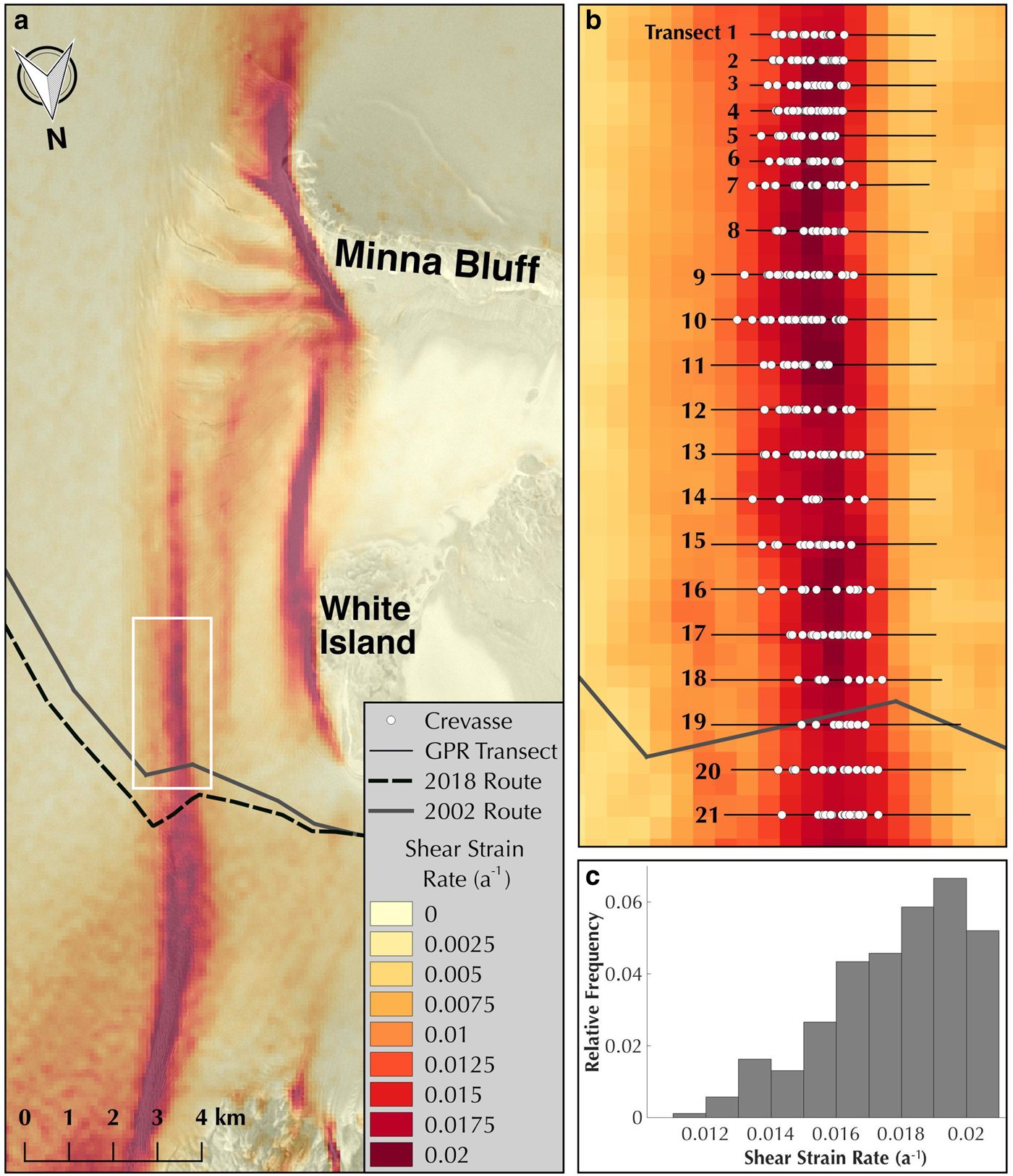
Fig. 3. (a) Gridded map of interpolated shear strain rate overlaid on Radarsat2 image. (b) Close-up of field area outlined in white in the overview panel. Gray lines indicate GPR transect routes with crevasses noted by white circles. (c) Plot of the relative frequency of crevasses with respect to shear strain rate. It is important to note that this is not a true histogram of crevasse observations, but the relative frequency of crevasse observations within a given bin (see Appendix B).

Fig. 4. Relative frequency distribution plots of shear strain rate, vorticity, dilatation, flow-parallel shear and flow-perpendicular shear, from MEaSUREs2 velocity data. Auto-RIFT plots are provided in Appendix A.
Results
A total of 420 crevasse features were identified from our GPR dataset. 333 of these features were simple slot crevasses and 87 were less distinct features interpreted as crevasses. Results presented in this section include all crevasse features. Table 1 includes the range of values of shear strain rate, vorticity and dilatation (derived from both the MEaSUREs2 and auto-RIFT velocity datasets) where crevasses were found.
Table 1. Range of values for kinematic outputs in m a−1 derived from the velocity data where crevasses were found. Auto-RIFT values were averaged from 2014 to 2017. Frequency distribution plots for MEaSUREs2 outputs can be found in Figure 4 and plots for auto-RIFT outputs are included in Appendix A.

Surface shear strain rates proved best for predicting crevasse features, with regions of higher shear strain rate more likely to have a greater number of crevasses (Fig. 4). Values of shear strain rate derived from the MEaSUREs2 velocity dataset range between 0.005 and 0.020 a−1 in the surveyed area of MSZ, with crevasses located at a minimum of 0.011 a−1. Interpolated rates of vorticity also show a correlation with crevasse location with vorticity magnitude values between 0.006 and 0.022 a−1 and crevasses located at a minimum of 0.013 a−1. Despite differences in horizontal resolution and time periods of acquisition, threshold values for shear strain rate and vorticity, as well as the shape of their relative frequency distribution plots, show good agreement between the MEaSUREs2 and averaged auto-RIFT datasets (Appendix A). However, dilatation estimates did not agree well between datasets, therefore no clear threshold value could be identified. No distinct spatial patterns in crevasse width or snowbridge thickness were found. We also evaluated each crevasse based on USAP's mitigation criteria for the MSZ region developed by the Cold Regions Research and Engineering Laboratory (CRREL): in order for a crevasse to be deemed safe to cross by a large tracked vehicle, its maximum width cannot exceed the thickness of its overlying snowbridge (Lever, Reference Lever2002). It is important to note that this criterion is only valid for the specific conditions of the MSZ. Based on this criterion we determined the crevasse width to snowbridge thickness ratio W max/H, which we will call aspect ratio for simplicity, for each crevasse (Fig. 5). While the aspect ratio of a crevasse has no real physical meaning, evaluating this ratio is useful for identifying whether or not a crevasse will need to be mitigated by USAP (i.e. opened and filled with snow when W max/H>1) during future traverses. Our crevasses show a pattern in which the relative aspect ratio of crevasses appears to increase in the southward direction.

Fig. 5. Plot of aspect ratio of each crevasse feature. Snowbridge thickness H was quantified as the distance from the glacier surface to the strongest peak of the hyperbola overlying the void. The minimum snowbridge thickness value was defined as the shallowest hyperbolic peak, while the maximum thickness was defined by the top of the void. Crevasses below the solid diagonal line would require remediation according to USAP's MSZ mitigation criterion.
Discussion
Implications for crevasse initiation
Our analysis suggests that flow in the MSZ is dominated by simple shear, as seen in the similarities between the relative distribution plots for flow-perpendicular shear, shear strain rate and vorticity. While the shear strain rate threshold proved to be the best criterion for predicting crevasse initiation in our study region, the dominant causal mechanism for crevasse formation is stretching in one or more directions. However, because our area of interest is dominated by simple shear, the direction of stretching is defined as a function of the shear strain rate. In areas of complex shear, this would not be the case and a crevasse initiation threshold based solely on shear strain rate would be inadequate.
In theory, one could apply the derived shear strain threshold to velocity outputs from future modeling scenarios of the MSZ to qualitatively predict how the crevasse field will evolve over time. Such an analysis would be useful for both logistical purposes (i.e. to determine which regions will be the most crevassed in the future) as well as scientifically for predicting changes in backstress due to either a decrease or increase in damage along the shear margin. However, crevasse initiation depends on density, crystallography, ice history and temperature, all of which may evolve with the crevasse field; therefore, some caution should be used when applying this shear strain threshold to forward modeling.
Implication on Shear Zone stability
Despite the clear evidence of a complicated history of ice deformation and fracture within our particular study site, the patterns from Figures 5 and 6 provide some insight into the current stability of the region. While the concept of the aspect ratio was conceived for safety purposes and the term has no direct physical meaning, it provides a first-order approximation of the ratio of the crevasse opening rate versus the accumulation rate in the snowbridge. We make two assumptions to arrive at this simplification: (1) the effect of snow compression due to bridging is negligible, and (2) crevasses form at the near surface. Although we cannot definitively rule-out that crevasses form at depth as discussed by Colgan and others (Reference Colgan2016), most evidence for initiation at depth is from theoretical work (Van der Veen, Reference Van der Veen1999; Nath and Vaughan, Reference Nath and Vaughan2003) or observations that are limited and/or unique in nature (Scott and others, Reference Scott, Smith, Bingham and Vaughan2010). For the MSZ region, the overwhelming majority of crevasse observations, including those from previous GPR campaigns that investigated to depths of ~170 m (Arcone and others, Reference Arcone2016), come from 0 to 20 m depth. Consequently, the crevasses in our study region likely form near the surface. If we also assume accumulation rate to be relatively constant, whereas opening rate depends on the stress state of each crevasse, then each point in Figure 5 indicates that particular crevasse's history. We thus interpret crevasses just above the horizontal axis of Figure 5 to be the youngest, because they are opening at a faster rate than they can be buried. Conversely, crevasses with thick snowbridges are interpreted as older. The lack of wide, deep crevasses (top right of the spectrum in Fig. 5) could indicate few relict crevasses, and that older crevasses have healed. Data in the top left of Figure 5 may be an example of older crevasses that have partially healed.
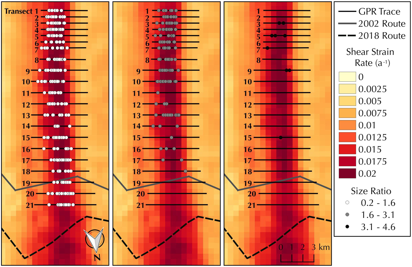
Fig. 6. Spatial pattern of differing aspect ratios of crevasse features. The aspect ratio increases in the southward direction (i.e. crevasses are wider with respect to their snowbridge thickness in the southern part of our survey).
While we did not find a strong spatial pattern in crevasse width or snowbridge thickness, the aspect ratio appears to increase in the southward direction (i.e. crevasses are wider with respect to their snowbridge thickness in the southern part of our survey, as seen in Fig. 6). This pattern could be due to several different reasons:
(1) our initial assumption of a spatially constant accumulation rate is inaccurate and in fact there is a pronounced increase in accumulation rate toward the south,
(2) crevasses have a greater opening rate toward the south,
(3) crevasses are opening quickly in the south and then healing as they advect northward and we only see newer, thinner crevasses on top, and/or
(4) there is a transient effect where crevasses are staying open for a longer period of time in the southern portion of our survey.
While local variations in accumulation rate are likely, we have found little evidence to support scenario 1. RACMO accumulation rate values are lower in the southern portion of the survey (Van de Berg and others, Reference Van de Berg, Van den Broeke, Reijmer and Van Meijgaard2006), while estimates from Arthern and others (Reference Arthern, Winebrenner and Vaughan2006) have the opposite spatial pattern with slightly higher estimates in the southern portion (on the order of mm). Scenario 2 is certainly plausible as the shear strain rate is generally higher in the southern portion of our survey. Scenario 3 is unlikely as repeat GPR surveys performed by SPoT from 2002 to 2016 along the road show little indication of crevasse healing, with all monitored crevasses continuing to widen from year to year. Scenario 4 would indicate the region is not in steady state and is in fact, changing over time.
Recent changes in ice flux have been observed both upstream and downstream of the MSZ that could affect the stress balance distribution within the region. Most notably, between 2016 and 2017, a previously inactive rift at the edge of the MIS widened and propagated over 3 km and eventually led to the calving of a 14 km2 tabular iceberg (Banwell and others, Reference Banwell2017). GPS-velocity measurements from 2016 to 2017 in the vicinity of the rift indicated a distinct change in direction in the wake of the calving event (MacAyeal, personal communication; see also Banwell and others, Reference Banwell, Willis, Macdonald, Goodsell and MacAyeal2019). These observed changes along the MIS front represent an important perturbation of the downstream boundary condition that could alter longitudinal stresses and velocity patterns within the MSZ. For example, this calving event could potentially drive longitudinal extension along the MIS due to a reduction in back-stress at the calving front. This in turn could cause a widening of the shear zone. Thus, both scenarios 2 and 4 seem the most likely and further observations of temporal variations in the spatial pattern of the aspect ratio are needed to definitely assess whether deviations in the flow field from steady state have an appreciable influence on crevasse opening and closure.
Viability of the South Pole Traverse
Since its creation in 2002, the South Pole Traverse route has advected ~4 km at its western edge and ~6 km at its eastern edge. The traverse route is now located in a region where the shear zone is wider. In addition, it has rotated ~40° and stretched ~1 km lengthwise, causing a greater portion of the traverse to be in a region that exceeds our threshold shear strain rate for crevasse initiation. Crevasse mitigation efforts have become more time-consuming as the number of crevasses that need to be mitigated have increased and USAP currently has plans to create a new route. This would suggest that the relative aspect ratio of crevasses along the road has increased over time, which is counter to our observations where the relative aspect ratio of crevasses appears to decrease in the northward direction. This discrepancy may be due to the fact that even the northern-most survey line is ~3.2 km to the south of the center of the current route crossing location and ~1 km north of where ice begins to flow around White Island and into the MIS. We therefore have limited observations of crevasses in this region where there is a considerable added effect from the flow-parallel shear component of the velocity field.
We identified the two most viable route locations between transects 14 and 15 and between transects 18 and 19 called Route 1 and 2, respectively. These two areas are located at local minima of both shear strain rate (Fig. 6) and the number of crevasses that would require remediation (Fig. 7) and were placed perpendicular to flow. To identify the ideal route from these two options, we advected the two routes over the next 20 years using the average velocity field from MEaSUREs2 and annually extracted the shear strain rate along each yearly route position (Fig. 8). To provide a first-order estimate of the number of crevasses along each route, we multiplied the relative frequency of crevasses from our distribution plots by the shear strain rate at 5 m spacing and summed the result (Fig. 9). We also compared the percent of the crossing that would be above the shear strain threshold for crevasses, which we estimate as 0.011 a−1 from our observations.
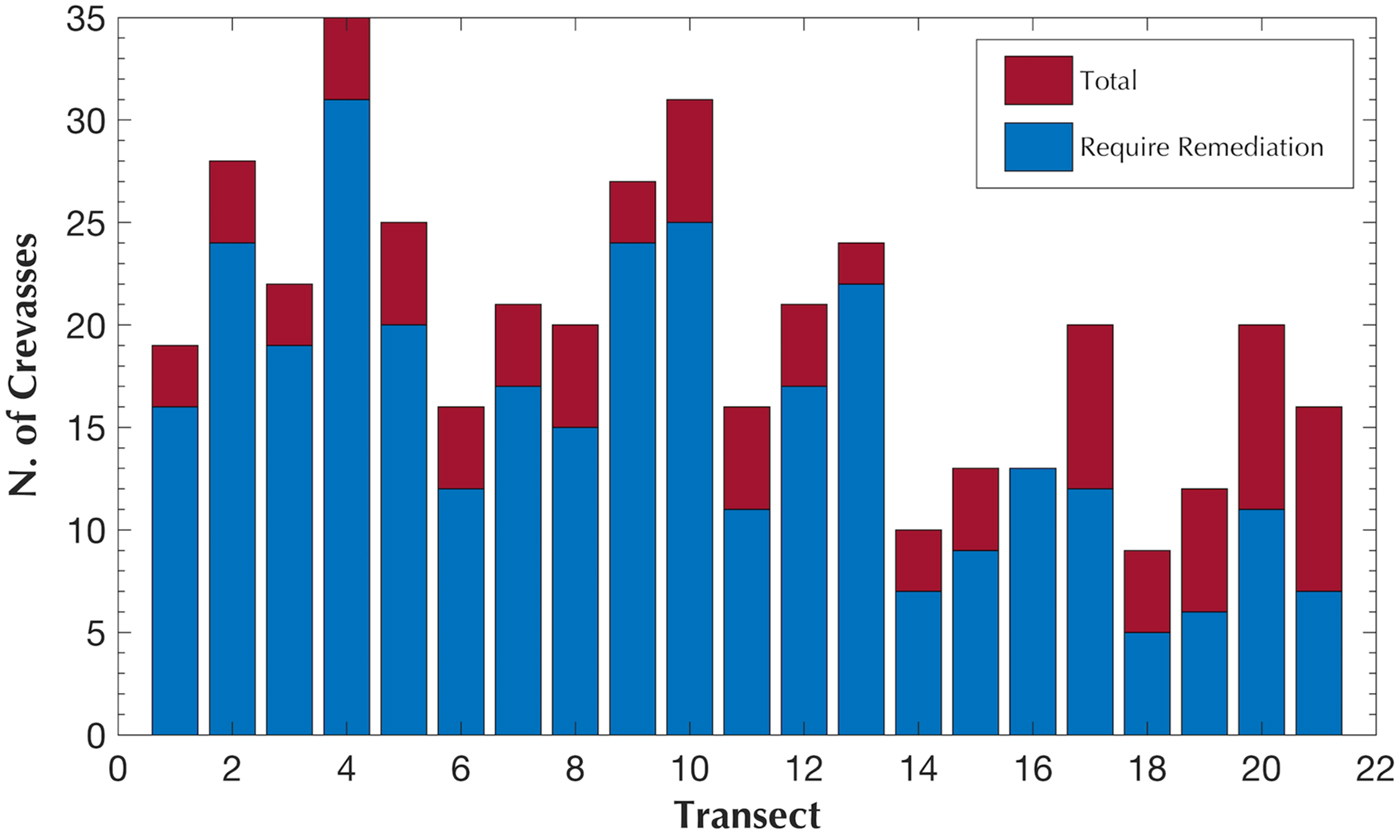
Fig. 7. Bar graph of the total number of crevasses located along each transect as well as the number of crevasses that would require remediation based on USAP's MSZ mitigation criterion.
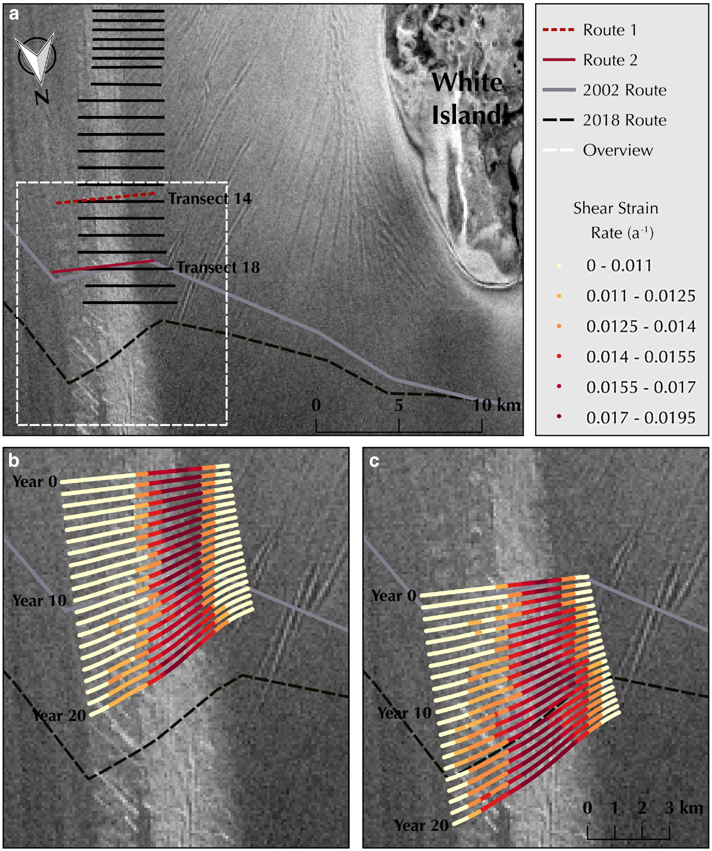
Fig. 8. (a) Radarsat2 image of the MSZ and White Island area. Potential Route 1 is noted by the dashed red line and potential Route 2 is noted by the solid red line. Overview of the bottom panels is outlined by the dashed white line. (b) Location and shear strain rate of Route 1 as it advects 20 years into the future. (c) Location and shear strain rate of Route 2 as it advects 20 years into the future. A greater portion of Route 2 is susceptible to crevassing due to the added component of flow-parallel shear as the route flows past the tip of White Island.

Fig. 9. (Top) Number of crevasses predicted for Route 1 and 2 as they advect 20 years. (Bottom) Percent of route above a shear strain threshold of 0.011 a−1.
Analysis of our dataset suggests the best location for a new route would be Route 1, ~9.3 km south of the midpoint of its current position and ~4.3 km south of the midpoint of its original location in 2002. This potential route would advect through a narrower portion of the shear zone than Route 2, which is located just to the south of where the shear zone begins to widen drastically due to the added component of flow-parallel shear as ice flows past the tip of White Island. In addition, Route 2 would likely be more susceptible to far-field changes along the MIS front. We therefore believe the traverse crossing would require less mitigation in the long-run if it is moved to the location of Route 1.
Conclusions
Our analysis suggests that flow in the MSZ is dominated by simple shear and that crevasse initiation typically occurs when the shear strain rate exceeds a value of 0.011 a−1 and vorticity magnitude of 0.013 a−1. Shear strain rate appears to be the best indicator for predicting crevasse locations, with regions of higher shear strain rate more likely to have a greater number of crevasses. The depth of snowbridge thickness and/or width of crevasses in the MSZ do not appear to correlate with the shear strain rate and/or vorticity. However, the aspect ratio of individual crevasses decreases in the northward direction of ice flow so that there are fewer wider and shallower crevasses toward the northern limit of our study site.
Although the method presented here provides a means to infer the presence or absence of crevasses in lateral shear zones with high-frequency radar observations, there are still several limitations to this method. First and foremost, our radar transects discretely sample the crevasse field and it is nearly impossible to identify all of the crevasses within each transect using either automated or manual methods. The spatial resolution of the radar data, as well as the remotely-sensed velocity data, may influence the derived crevasse initiation threshold. The quality and spatio-temporal sampling of the velocity dataset will also influence the analysis.
As previously stated, crevasse initiation depends on several factors including ice temperature, density, crystallography and ice history. Therefore, the threshold values derived for the MSZ cannot be directly applied to other glacial environments. However, a similar shear strain threshold value should be applicable in other areas dominated by simple shear, and the method provided here can be repeated to find other kinematic threshold criteria for more complex shear margins, to study shear margin evolution, and to assess localized damage and weakening processes in locations using minimal in situ data.
Contribution statement
SA conceived the project idea, the fieldwork plan and modeling portion of which were greatly refined by GH and PK. GH and PK acquired funding and provided project administration. LK took the lead on data acquisition, curation, formal analysis, methodology and investigation with supervision from GH, PK and EE during different stages of the research; SA and ZC assisted with the data processing and interpretation. LK wrote the manuscript and all authors, apart from GH, provided critical feedback on revisions.
Acknowledgments
This paper is dedicated to the memory of Gordon Hamilton who died while performing fieldwork in a crevassed portion of the McMurdo Shear Zone. Gordon's innovative ideas and mentorship provided the foundation for this work, and we hope this paper will contribute to the safety of scientists conducting fieldwork in hazardous regions.
This work was funded by the US National Science Foundation grant ANT-1246400 awarded to Hamilton, Koons and Laura Ray. We would like to especially thank Ray and James Lever for their contribution to project conceptualization and administration as well as our other Dartmouth collaborators Benjamin Walker, Joshua Elliot and Austin Lines for the design and operation of robotic rovers in the field. Sincere thanks are given to Alex Gardner for providing JPL auto-RIFT velocities and solving data quality issues. We would also like to thank Peter Braddock for assistance in the field as well as Seth Campbell who contributed to both fieldwork and scientific discussions. We would like to thank the South Pole Traverse team for their logistic support that made our study possible. We are also grateful to Martin Truffer for helpful comments throughout the writing process as well as Alison Banwell and one anonymous reviewer for their thorough and helpful comments during the review process.
Appendix A: Auto-RIFT outputs
Here we present results from the auto-RIFT derived velocities (Fig. 10). While kinematic outputs were derived on a yearly basis from 2014 to 2017 m a−1, we found the best results by averaging these years together. Threshold values for shear strain rate and vorticity show good agreement with MEaSUREs2 values despite differences in horizontal resolution and time periods.
Fig. 10. (a) Relative frequency distribution plots of shear strain rate, vorticity and dilatation, from auto-RIFT velocity data.
Appendix B: Relative frequency distribution normalization
The purpose of this section is to provide details on the subtleties of the relative frequency distribution plots in Figures 3c and 4. It is important to note that these plots are not histograms of crevasse observations, but the relative frequency distribution of crevasses within a given bin. For example, Figure 3c should not be interpreted to mean that 7% of crevasses occur between a shear strain rate of 0.019–0.020 a-1, but rather that 7% of all observations within a shear strain rate of 0.019–0.02 a-1 are crevassed. Figure 11 provides a histogram of crevasse observations without normalization and a histogram of all observations; the division of the two provides the normalized plot in Figure 3c.
Fig. 11. (Top) Histogram of crevasse observations. (bottom) Histogram of all observations.


 Open access