


1. Introduction
The importance of oceanic mesoscale eddies in maintaining general circulation of the global ocean is well established (McWilliams Reference McWilliams2008). In oceanic general circulation models (OGCMs), the most accurate way to account for the eddy effects is to resolve them dynamically as finely as possible given the computational constraints. This route is computationally expensive and not feasible for many practical applications, including climate system modelling. However, there is general hope that, in non-eddy-resolving and eddy-permitting OGCMs, some large-scale circulation component can be modelled dynamically whereas the effects of the remaining mesoscale-eddy circulation component can be somehow parameterized (i.e. represented by simple, parametric mathematical models) in a satisfactory way. Along this line, the ocean circulation problem is especially difficult if compared with other turbulence problems needing parameterizations because the involved eddy/large-scale interactions are controlled by both forward and backward energy cascades and non-local transfers, all operating in the presence of significant large-scale spatial inhomogeneities and low-frequency variabilities (e.g. Aluie, Hecht & Vallis Reference Agarwal, Ryzhov, Kondrashov and BerloffReference GroomsReference Aluie, Hecht and Vallis2018). Therefore, active research on developing efficient and accurate eddy parameterizations, for example, for climate modelling, will be in demand for the foreseeable future, and the main need for the parameterizations will drift towards the eddy-permitting models, as progressively finer grid resolutions become affordable.
There is no need to review here the massive and rapidly growing literature on eddy parameterizations because details of the existing approaches are not directly relevant to our study, which deals with the general and fundamental problem of sorting out dynamically resolved and unresolved eddy components. For a big picture on various parameterization approaches, we refer readers to the introduction in Klower et al. (Reference Klower, Jansen, Claus, Greatbatch and Thomsen2018). Most of the eddy parameterization approaches are diffusive, that is, based on the assumption that eddy fluxes are linearly related to the corresponding large-scale gradients. An alternative approach (Ryzhov et al. Reference Ryzhov, Kondrashov, Agarwal and Berloff2019, Reference Ryzhov, Kondrashov, Agarwal, Berloff and McWilliams2020) is to emulate eddies statistically and input them into non-eddy-resolving models. Note, that either approach needs information about the unresolved eddy field, hence, defining the latter becomes important and may strongly influence the resulting eddy parameterizations. Having said this, we stay within an idealized model set-up, develop a novel methodology for finding the unresolved eddy component as the field error followed by its subsequent analysis and explain the advantages of this approach.
In this paper we deal with the following pair of long-standing theoretical problems that hamper progress in eddy parameterizations. The first problem is the existing broad uncertainty in defining the eddies, that is, in deciding on how to decompose a turbulent flow into its large- and small-scale (hereafter, eddy) components. For mesoscale oceanic eddies of this problem remains generally unresolved for several reasons. First, there is no significant spectral gap between the length (and also time) scales of the flow patterns, hence, separation of the large- and small-scale components becomes spectrally ambiguous (Wunsch & Stammer Reference Wunsch and Stammer1995; Stammer Reference Stammer1997; Wunsch Reference Wunsch2009). Also, geographical variations of the involved scales are significant and further complicate applicability of spectral decompositions, which are spatially non-local but local spectrally. Second, there is neither unique nor objectively constrained flow decomposition based on some local filtering of the full flow (Leonard Reference Leonard1975; Sagaut Reference Sagaut2006), as we do not know how to select objectively properties of the filters. On the other hand, we know that the dynamics of the length scales corresponding to less than approximately 10 grid intervals is misrepresented (e.g. Karabasov, Berloff & Goloviznin Reference Karabasov, Berloff and Goloviznin2009), but it is hard to be more precise, and it is even harder to translate this information into practical decisions about the filtering. This misrepresentation increases with progressively decreasing scales within the corresponding ‘grey zone’ of the partial resolution, until all scales shorter than the nominal resolution of the model grid become missing in the dynamics. The above issues alone make objective flow decomposition difficult but the situation is actually even worse because the nonlinear interactions tangle together the involved length (and also time) scales, which can be widely incommensurate: for example, non-local inverse cascades (Scott & Wang Reference Scott and Wang2005) and intrinsic eddy-driven low-frequency variability (Berloff, Hogg & Dewar Reference Berloff, Hogg and Dewar2007). This tangling implies that the ‘grey zone’ of the partial resolution may extend far into the nominally resolved scales (i.e. into the scales approximately equal to and even much longer than 10 grid intervals). Furthermore, different dynamical variables may have widely different scales (e.g. pressure and relative vorticity), implying that the corresponding eddies may be filtered out differently, thus bringing in extra complexity.
The second long-lasting theoretical problem is that we do not know how to separate dynamically resolved and unresolved eddy field components, as only the latter actually needs to be parameterized. In other words, there are no satisfactory connections between the existing local flow decompositions (i.e. filtering) and the numerical, non-eddy-resolving or eddy-permitting models employed to simulate the large-scale flow component provided that the eddy effects are somehow parameterized. In other words, we do not know how to make an eddy filtering consistent with (and ideally unique for) the applied coarse-grid model dynamics. This problem is generally recognized, but attempts to resolve it remain largely empirical; e.g. by relating coarse-grid resolution to the first baroclinic Rossby radius (Hallberg Reference Hallberg2013), which is loosely taken as the eddy filtering scale. Although, the first Rossby radius is a reasonable first guess due to its relation to the ubiquitous baroclinic instability mechanism maintaining most of the eddies (Pedlosky Reference Pedlosky1987), the ocean circulation has many other operating length scales that complicate the issue.
Let us now discuss closely related local eddy filtering studies of the ocean (e.g. Berloff Reference Berloff2015, Reference Berloff2016, Reference Berloff2018; Zanna et al. Reference Zanna, Mana, Anstey, Tomos and Bolton2017; Aluie et al. Reference Aluie, Hecht and Vallis2018) and some other types of turbulence (e.g. Piomelli et al. Reference Piomelli, Cabot, Moin and Lee1991; Vreman, Geurts & Kuerten Reference Vreman, Geurts and Kuerten1994). In these works, despite the inherent uncertainty about knowing the right one, each filter, except for the classical (and most common in geophysics) Reynolds flow decomposition into the time mean and fluctuations, allows both the large-scale and eddy flow components to have spatio-temporal variabilities. Non-Reynolds filterings for defining and dealing with the flow components are much more suitable for the eddy parameterization problem because, ultimately, we need coarse-grid models to be capable of predicting time-dependent flows rather than steady-state balances (as would be in the Reynolds case). Apart from having this clear advantage, the local filterings are not yet capable of resolving the outlined long-lasting theoretical problems.
The above-discussed theoretical problems motivate us to redefine the object for parameterization by starting from the coarse-grid dynamics, rather than choosing an eddy filter, and finding what is missing in it, in terms of the field error. The latter object can be viewed as the ‘virtual eddy field’, which is the primary object for parameterization, and the process of finding it can be viewed as reconstruction of the dynamically unresolved flow. Given that the term ‘eddies’ is ambiguous and has many meanings, we could refer to the new object as the dynamical (rather than directly observed) eddy field, but we opted out to be conservative with the terminology. More specifically, we will employ a coarse-grid dynamical model, augment it by adding some interactive error-correcting forcing (ECF), so that it reproduces the (observed) reference flow, and translate the ECF history into the corresponding field error. This process can be viewed as a flow unfiltering, in which the coarse-grid model plays a role of the filter and reconstructs the missing component of the flow. The explicit dependence of the flow reconstruction on the coarse-grid model takes into account its formulation, configuration and numerical implementation (e.g. computational grid and algorithms). There have been a few attempts to achieve this, and the approach taken by Berloff (Reference Berloff2005a,Reference Berloffb) can be considered as a precursor to the present study. In that work, the residual between the observed reference flow and the coarse-grid model solution was treated as the eddies and used to construct the eddy forcing, correcting the nonlinear terms in the coarse-grid model. Along this general line, some earlier studies used a truncated approximation of the Navier–Stokes equation solved on a finer grid (Domaradzki, Loh & Yee Reference Domaradzki, Loh and Yee2002), calculated residual eddy forcing from the tendency term (D'Andrea & Vautard Reference D'Andrea and Vautard2000) and even used the residual eddy forcing to correct the eddy diffusivity coefficient (Kaas et al. Reference Kaas, Guldberg, May and Deque1999). The other approach that has clear connection to our work is approximate deconvolution-based reconstruction of the eddies and their effects in the coarse-grid model (San, Staples & Iliescu Reference San, Staples and Iliescu2011, Reference San, Staples and Iliescu2013). In all these studies the residual eddy forcing corrections were imperfect, hence the coarse-grid models could not reproduce the benchmark reference flows exactly.
Having discussed the relevant background information, we are now ready to state that, within the quasigeostrophic approximation, the main objectives of this paper are: (i) to propose a way towards resolving both of the above-discussed long-standing fundamental problems by filtering the field errors dynamically and by showing their statistical robustness; (ii) to identify the main statistical and dynamical properties of the resulting field errors; and (iii) to demonstrate that they are significantly different from the locally filtered eddies, (iv) to argue that the field errors can be emulated and closed on the dynamically resolved flow and the resulting ECF for the model augmentation can be the ultimate product of future eddy parameterizations. The paper is organized as follows. Section 2 outlines the employed ocean model, § 3 explains the methodology for dynamical filtering of the eddies and § 4 provides and analyses phenomenology of the eddies and their eddy forcing, and also makes comparisons with locally filtered eddies. Finally, we summarize and discuss the results in concluding § 5.
2. Ocean model
The dynamical model and its reference solution are extensively discussed in Ryzhov et al. (Reference Ryzhov, Kondrashov, Agarwal and Berloff2019). Therefore, here we just remind the reader that the focus is on the classical wind-driven, double-gyre quasigeostrophic potential vorticity (PV) model representing a midlatitude ocean circulation, such as in the North Atlantic and North Pacific. The model is configured in a flat-bottom square basin aligned with the usual zonal and meridional coordinates, and filled up with 3 stacked isopycnal fluid layers. The governing equations for the layer-wise PV anomalies  $q_i$ and velocity streamfunctions $\psi _i$ are
 $$\begin{gather} \frac{\partial {q_1}}{\partial {t}} +J(\psi_1,q_1) +\beta \frac{\partial {\psi_1}}{\partial {x}} = W(x,y) +\nu \nabla^{4} \psi_1 , \end{gather}$$
 $$\begin{gather}\frac{\partial {q_2}}{\partial {t}} +J(\psi_2,q_2) +\beta \frac{\partial {\psi_2}}{\partial {x}} = \nu \nabla^{4} \psi_2 , \end{gather}$$
 $$\begin{gather}\frac{\partial {q_3}}{\partial {t}} +J(\psi_3,q_3) +\beta \frac{\partial {\psi_3}}{\partial {x}} ={-}\gamma \nabla^{2} \psi_3 +\nu \nabla^{4} \psi_3 , \end{gather}$$
 $$\begin{gather}q_1 =\nabla^{2} \psi_1 + S_{1} (\psi_2 -\psi_1) , \end{gather}$$
 $$\begin{gather}q_2 =\nabla^{2} \psi_2 +S_{21} (\psi_1 -\psi_2) +S_{22} (\psi_3 -\psi_2), \end{gather}$$
 $$\begin{gather}q_3 = \nabla^{2} \psi_3 + S_{3} (\psi_2 - \psi_3) , \end{gather}$$
where the layer index  $i$ starts from the top, and $J(\cdot ,\cdot )$ is the Jacobian operator. We are confident that the approach proposed in this study is directly applicable to any other quasigeostrophic model (e.g. single gyre or two-dimensional turbulence), because the employed baroclinic double-gyre model is the most complicated one in the hierarchy of the common quasigeostrophic models, due to its lack of spatial symmetries. However, a follow-up extension of the approach to the primitive equations (used in comprehensive OGCMs) remains to be worked out.
The main parameters of the ocean model are as follows: the basin size is  $L = 3840$ km; the layer depths at rest are $H_1 = 0.25$ km, $H_2 = 0.75$ km and $H_3 = 3.0$ km; $\beta = 2\times 10^{-11}$ m $^{-1}$ s $^{-1}$ is the midlatitude planetary vorticity gradient; $\nu = 2$ and $50$ m $^{2}$ s $^{-1}$ are the eddy viscosity values used in the eddy-resolving and coarse-grid model configurations, respectively; $\gamma = 4\times 10^{-8}$ s $^{-1}$ is the bottom friction parameter; the stratification parameters $S_1$, $S_{21}$, $S_{22}$ and $S_3$ are chosen so that the first and second baroclinic Rossby deformation radii are $Rd_1 = 40$ km and $Rd_2 = 20.6$ km, respectively; and $W(x,y)$ is the asymmetric, steady, double-gyre wind curl (Ekman pumping) forcing
 $$\begin{gather} W(x,y) ={-}\frac{{\rm \pi} \tau_0 A}{L} \sin \left[ \frac{{\rm \pi} (L+y)}{L +B x} \right] , \quad y \le B x , \end{gather}$$
 $$\begin{gather}W(x,y) ={+}\frac{{\rm \pi} \tau_0}{L A} \sin \left[ \frac{{\rm \pi} (y -B x)}{L -B x} \right] , \quad y > B x , \end{gather}$$
where the asymmetry parameter is  $A = 0.9$, the non-zonal tilt parameter is $B = 0.2$ and the wind stress amplitude is $\tau _0 = 0.08$ N m $^{-2}$. Overall, the asymmetrically forced flow regime is close to the one considered by Rhines & Schopp (Reference Rhines and Schopp1991). The layer-wise model (2.1)–(2.6), with the added partial-slip lateral boundary conditions and mass conservation constraints, are solved numerically (Karabasov et al. Reference Karabasov, Berloff and Goloviznin2009).
For each reference solution, the model was spun up from the state of rest until the statistical flow equilibration was reached. Then, it was run for 100 years, with the solution saved either every day or every hour (depending on the type of analysis to be carried out) and used later for various analyses within our study. In practice, as discussed later on, we saved the solution slightly before and after the reference time of each record, because of the need to estimate the PV tendency term at each reference time. The exact values of PV anomalies and streamfunctions at the reference times are obtained by simple arithmetic averages of the before and after fields. The model solutions were obtained on the uniform, fine (eddy-resolving) and coarse (non-eddy-resolving) grids. The former grid has  $513^{2}$ nodes with 7.5 km nominal resolution, whereas the latter grid has $129^{2}$ nodes with 30 km nominal resolution. The coarse-grid resolution can be characterized as eddy permitting because the grid interval is slightly shorter than the first baroclinic Rossby radius of deformation (40 km). In Appendix A extending the main results, we provide analyses for the coarse-grid model with a non-eddy-resolving grid characterized by 60 km nominal resolution and $65^{2}$ grid points.
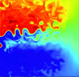
The flow solutions are characterized by the instantaneous and time-mean fields, and the latter is denoted by angle brackets  $\langle \cdot \rangle$. The reference eddy-resolving solution (the solution is numerically converged and its robustness relative to progressively increasing Reynolds number has been explored elsewhere (Shevchenko & Berloff Reference Shevchenko and Berloff2015, Reference Shevchenko and Berloff2017)) (figure 1) is characterized by the well-developed eastward jet extension of the western boundary currents and its adjacent recirculation zones. These are the main flow features that fade away when the eddies are not resolved properly. This can be seen from the benchmark, coarse-grid reference solution (figure 1d–f). The eastward jet in the eddy-resolving solution is tilted away from the zonal direction, and the gyres are significantly asymmetric, all due to the deliberately imposed asymmetry of the wind forcing $W(x,y)$, which makes the flow regime both more generic and resembling of the actual eastward Gulfstream extension. The imposed asymmetry in combination with the fine grid resolution and high Reynolds number (due to the low eddy viscosity value) make the explored flow regime qualitatively and quantitatively different from the classical double-gyre solutions obtained with early models (e.g. Holland Reference Holland1978) and more similar to the ones studied by Rhines & Schopp (Reference Rhines and Schopp1991). The deep-ocean eddy-resolving solution is characterized by the large pool of nearly homogenized PV in accord with the other eddy-resolving double-gyre studies and PV homogenization theory (Young & Rhines Reference Young and Rhines1982; Holland, Keffer & Rhines Reference Holland, Keffer and Rhines1984). The nonlinear eddy/large-scale interactions and the involved dynamical mechanism acting in the reference eddy-resolving solution are not discussed here; the readers are referred to the other relevant studies (e.g. Berloff et al. Reference Berloff, Hogg and Dewar2007; Shevchenko & Berloff Reference Shevchenko and Berloff2016, Reference Shevchenko and Berloff2017; Berloff Reference Berloff2018).

Figure 1. Reference eddy-resolving and coarse-grid double-gyre model solutions. Top row shows the eddy-resolving upper-ocean fields: instantaneous snapshots of (a) PV anomaly  $q_1$ and (b) velocity streamfunction $\psi _1;$ and (c) time-mean $\langle \psi _1 \rangle$. Middle row shows the same but for the coarse-grid model (without any augmentation by the eddy forcing). Note that the coarse-grid model fails to simulate the eastward jet extension of the western boundary currents with its adjacent recirculation zones. Deep-ocean eddy-resolving flow is illustrated by the corresponding snapshot of PV anomaly $q_2$ in panel (g). The difference between the time-mean circulations in panels (c, f) is plotted in panel (h) – this is the missing time-mean part of the circulation due to the unresolved eddy effects. Panel (i) shows the same as (h), but for the deep-ocean flow in the middle isopycnal layer; note that the coarse-grid modelled eastward jet is missing in the deep ocean as well. Units of the plotted fields are non-dimensional, with the length scale $L=30 \times 10^{5}$ cm (the coarse grid interval) and velocity scale $U=1.0$ cm s $^{-1}$. These units are consistently used across all figures in the paper.
Note that the eddy viscosity values in the coarse-grid and eddy-resolving models are different, but this difference is neither required nor essential for the dynamical eddy filtering procedure explained further below. In this procedure the augmented coarse-grid model can be stably computed with any eddy viscosity value, as it is always steered towards the reference flow and does not run away from it. However, if the eddy viscosity value were too low, the non-augmented coarse-grid model solution would develop large numerical errors. This is mostly because of the model's failure to resolve the viscous western boundary layer that significantly controls the whole flow regime (Berloff & McWilliams Reference Berloff and McWilliams1999b). Here, the benchmark coarse-grid model solution (figure 1d–f) was obtained with the safely large eddy viscosity value, and its failure to simulate the eastward jet and its adjacent recirculation zones is due to the unresolved and underresolved eddy effects only.
In the next section we will find what is missing in the coarse-grid dynamics and use this information to obtain the field errors.
3. ECF and reconstructed field errors
This central section of the paper discusses the residual ECF and dynamically reconstructed field errors. Note that the latter object can be viewed as dynamically unresolved eddies, which can be nevertheless represented on the coarse grid, whereas the former can be viewed as the corresponding eddy forcing. We start by coarse graining (i.e. projecting) the streamfunction of the eddy-resolving solution into the reference flow, which we call the ‘reference true flow’, or for the sake of brevity simply the ‘truth’ (further below we omit the quotation marks). This terminology should be viewed not as an overstatement but just as convenient labelling that reminds us that the reference flow is treated as both a set of exact observations (here, at the coarse-grid nodes) and the testing benchmark for the follow-up analyses. Note, since we do not apply any local filtering, the true reference flow has a maximum of the original information content as can possibly be given on the coarse grid. In order to project the original fine-grid information onto the coarse grid, we simply subsample the data, but, in principle, we could also use local averages over the fine-grid nodes contained within the coarse-grid cells. As we show later on, such small modifications of the reference flow have small effects on the outcome. No smoothing in time was applied, for simplicity, although this would be straightforward to implement. After the coarse graining was carried out, the resulting layer-wise streamfunctions were corrected by small constants, which ensure that the mass conservation constraints built into the ocean model (Karabasov et al. Reference Karabasov, Berloff and Goloviznin2009) are exactly satisfied. Once the corrected streamfunction is obtained, the corresponding layer-wise PV anomaly fields are obtained from it by the differentiation in accord with (2.4)–(2.6) rather than by applying separate coarse graining to the original PV anomaly field. This guarantees that both coarse-grained streamfunction and PV fields are consistent with each other.
3.1. Eddy forcing and ECF
In this section we discuss traditional and novel approaches for defining the eddy forcing term in the large-scale dynamical equation provided that some reference flow can be decomposed into some large-scale truth (indicated by overbars) and eddies (indicated by primes)
 \begin{equation} q(t,x,y,z)=\bar{q}+q' , \quad \psi(t,x,y,z)=\bar{\psi}+\psi' , \end{equation}
where the corresponding PV anomalies and velocity streamfunctions are related via the PV inversion (2.4)–(2.6). We assume here that everything so far happens on the fine grid, no coarse graining is involved, and later on the resulting eddy forcing will be related to the ECF. Note that, in general, both  $\bar {q}$ and $q'$ have projections on the coarse grid; therefore, a projection of the former component does not represent projection of the full field $q$. This is apparent loss of information provided that the ultimate goal is to model $\bar {q}$ on the coarse grid and parameterize effects of $q'$. The starting point is the basic quasi-geostrophic dynamics, and here we focus on the upper layer and omit the layer index for simplicity
 \begin{equation} \frac{\partial q}{\partial t} +J(\psi,q) +\beta \frac{\partial \psi}{\partial x} = \nu \nabla^{4} \psi +W . \end{equation}
The next goal is to obtain a prognostic equation for  $\bar {q}$, and for convenience we restrict the upcoming discussion to the PV anomaly, keeping in mind that the streamfunction is always inverted from it. Let us now consider the traditional filtering approach (e.g. Sagaut Reference Sagaut2006), in which the overbar indicates some localized spatial filtering $\bar {\,\cdot \,}$ used to obtain the large-scale component in (3.1a,b), and apply the filtering to the governing equation (3.2)
 \begin{equation} \frac{\partial \bar{q}}{\partial t} +J(\bar{\psi},\bar{q}) +\beta \overline{\frac{\partial \psi}{\partial x}} =\nu \overline{\nabla^{4} \psi} +\bar{W} +[ J(\bar{\psi},\bar{q}) -\overline{J(\psi,q)}] . \end{equation}
Note that, in the above equation, the filtering does not have to commute with the spatial derivatives (e.g. when the filter width varies in space). The term in the square brackets here is referred to as the eddy forcing and denoted as
 \begin{equation} EF^{(1)}=J(\bar{\psi},\bar{q}) -\overline{J(\psi,q)} , \end{equation}
where the superscript indicates that this is the first eddy forcing expression, which corresponds to the filtering approach. Equation (3.3) is diagnostic for  $EF^{(1)}(t,x,y,z)$, and for this to happen it needs all 3 inputs: $\bar {q}$, $q'$ and $\bar {\,\cdot \,}$ (i.e. both the large-scale and eddy components, as well as the filter shape). On the other hand, if we treat this equation differently and aim to find $q'$, given the other 3 inputs – $EF^{(1)}$, $\bar {q}$ and $\bar {\,\cdot \,}$ – then, we are stuck, because unfiltering the Jacobian makes the whole effort numerically expensive and highly problematic, if not infeasible. To summarize, not only does traditional filtering have inherent loss of information, but also it does not easily allow us to recover eddies from the eddy forcing.
Let us now consider the alternative decomposition approach, which better fits our purposes. For this we substitute (3.1a,b) into (3.2) and rearrange the terms
 \begin{align} &\frac{\partial \bar{q}}{\partial t} +J(\bar{\psi},\bar{q}) +\beta \frac{\partial \bar{\psi}}{\partial x}=\nu \nabla^{4} \bar{\psi} +\bar{W}\nonumber\\ &\quad +\left[{-}J(\bar{\psi},q') -J(\psi',\bar{q}) -J(\psi',q') -\frac{\partial q'}{\partial t} -\beta \frac{\partial \psi'}{\partial x} +\nu \nabla^{4} \psi' +W'\right] . \end{align}
Compare this equation with (3.3) and note that it contains a different expression for the eddy forcing (in square brackets)
 \begin{equation} EF^{(2)} ={-}J(\bar{\psi},q') -J(\psi',\bar{q}) -J(\psi',q') -\frac{\partial q'}{\partial t} -\beta \frac{\partial \psi'}{\partial x} +\nu \nabla^{4} \psi' +W' . \end{equation}
Note, that the eddy forcing definitions are equivalent if the filtering commutes with the spatial derivatives. Let us assume this for our purposes. There is also a mismatch between  $\bar {W}$ and $W$ in the governing equations but it can be easily absorbed into one of the eddy forcing definitions (plus, in our case, it is very small because the wind forcing is essentially a smooth large-scale function). Thus, up to a close approximation (that can be easily dealt with and can change none of our conclusions and methods), we have: $EF^{(1)}=EF^{(2)}=EF$. Note that (3.6) is also diagnostic for $EF$, given $\bar {q}$ and $q'$, but it does not need any additional information on the filter shape. This is an advantage because (3.6) can be now solved for $q'$, given $EF^{(2)}$ and $\bar {q}$ – this is what we need for our purposes. To summarize, the decomposition approach still has the inherent problem of the loss of information but now it allows us to find the eddies given the eddy forcing, and there is no need to know the filter.
Suppose that we have a situation (3.5) for the grid that we consider as a coarse one, indicated by subscript ‘ $c$’. Also, let us now assume that the filtered field $\bar{q}$ is known as the large-scale flow component but the exact filter shape is not known, and the full flow is also not known. In other words, let us take $\bar {q}=q$, where the latter is the reference ‘true’ flow field projected on the coarse grid. Then, we can write down (on the coarse grid, as indicated by subscript ‘ $c$’) the following equations:
 \begin{equation} \frac{\partial \bar{q}}{\partial t} +J_c(\bar{\psi},\bar{q}+\beta y) =\nu \nabla_c^{4} \bar{\psi} +\bar{W} +EF_c(t,x,y), \end{equation}
and
 \begin{equation} \frac{\partial q'}{\partial t} +J_c(\bar{\psi},q') +J_c(\psi',\bar{q}) +J_c(\psi',q'+\beta y) -\nu \nabla_c^{4} \psi' -W' ={-}EF_c(t,x,y) . \end{equation}
Note that, despite similarities of these equations with (3.5) and (3.6), there are fundamental differences now: both equations are formulated on the coarse grid; all overbarred fields are the ‘true’ reference fields projected on the coarse grid; there is no explicit information on the filtering applied; and the primed fields are the unknown quantities to be found. Next, (3.7) can be used to find the eddy forcing (from the overbarred input), and now we refer to it as the ECF. This change of notation is justified by the fact that EF deals with real eddies, which are a component of the reference flow, whereas ECF deals with field error, which is reconstructed on top of the reference flow. The corresponding ECF can be used as the input for (3.8) to find the  $q'$ eddies, which we refer to as the field errors (and the corresponding streamfunction $\psi '$ is found by the inversion). Note that no information on the filter shape was ever needed, and this is the fundamental advantage of the whole approach. Instead of starting from the full flow and filtering it out into the large-scale and eddy components, we started from the full flow declared as the large-scale field and used the coarse-grid model to reconstruct the field error, which is not a physical object despite being a viable alternative to previously used decomposition approaches. Let us stress that, in the classical flow decomposition scenario, the starting point is some given $q;$ then, $\bar {q}$ is found by a filtering and $q'$ is found as the residual. In the approach proposed in this paper, the starting point is some given $\bar {q};$ then, $q'$ is found dynamically and $q$ is found as the sum of both. Note, however, that in the classical approach $q$,
$q$,  $\bar {q}$ and $q'$ exist as functions on the high-resolution grid, while in the new approach they only exist on the coarse-model grid.
We solved (3.7) for each layer over the full record (100 years) of the reference ‘truth’, and the resulting ECF solution was saved daily (or hourly), as needed for further analyses. In practice, we estimated the time derivative in (3.7) with the centred finite difference of the true PV anomaly. The other option to obtain the same (up to numerical errors) result is to integrate the coarse-grid model over a short time interval to find the corresponding residual from the truth and to divide this residual by the time interval, so that the resulting mid-interval ECF is evaluated. We tested this option and report here that it can be more practical for significantly more complicated, comprehensive OGCMs. For both algorithms, we found that the resulting ECF is insensitive to the time interval, as long as it is less than approximately 2 h – this value can be interpreted as the temporal resolution requirement for the time derivative in the ECF dynamics discussed further below. Finally, the ECF is cubically interpolated in time for further purposes, such as the time integration of the augmented coarse-grid model or solving for the field errors.
The resulting ECF field (figure 2) is characterized mostly by the nearly grid-scale anomalies in the immediate vicinity of the meandering eastward jet and most prominent vortices, and also located along the basin boundaries. This is expected because the coarse-grid derivatives have the largest errors on steep gradients, which characterize all these flow features and locations. We also note that some of the same-sign ECF anomalies are organized in groups spanning several grid intervals – this indicates the multi-scale nature of the field to be taken into account by eddy parameterizations. The main difference between the upper- and deep-ocean ECFs is mostly in terms of the magnitude, which tends to decrease with depth by one order of magnitude. We note that the ECF can be decomposed into rigorously defined components with specific dynamical meanings in accord with (3.8). In order to do this, first, we have to find the field errors, therefore, this analysis is deferred to § 4.2.

Figure 2. The ECF augmenting the coarse-grid model towards the reference true flow. Top row shows fields describing the upper-ocean ECF: (a) instantaneous snapshot, (b) time mean and (c) standard deviation. Bottom row shows the same but for the deep-ocean ECF. The zonal and meridional distances along the basin boundaries are as in figure 1, and are not shown from here on.
The governing coarse-grid field error model (3.8) can be viewed as the original quasigeostrophic dynamics that was modified as follows: (i) it is augmented with the additional Jacobians  $J(\bar {\psi }_i, q'_i)$ and $J(\psi '_i, \bar {q}_i)$, which involve advection of the field error PV anomaly by the large-scale flow, and advection of the reference PV anomaly by the field error; and (ii) it is driven by the ECF history instead of the wind curl $W(x,y)$. Note that the field error dynamics is fully nonlinear, and its linearized properties are fundamentally different from the classical linearization around the state of rest, due to the large-scale flow effects imposed via the additional Jacobians. It is worth noting the difference between (3.8) and the approach taken in Berloff (Reference Berloff2005a,Reference Berloffb), where only the Jacobian terms were taken into account in defining the eddy forcing of the coarse-grid dynamics, and the eddies were defined as the residual between the reference flow and the coarse-grid model solution. Note that, for (3.8), the implemented boundary conditions, mass constraint and elliptic PV inversion problem are the same, as in the original double-gyre model (§ 2; Karabasov et al. Reference Karabasov, Berloff and Goloviznin2009), and each involved equation is discretized and solved on the coarse grid, and with the same numerical methods.
There is a subtlety with the initial conditions for (3.8), and it is worth discussing here. For the reference field error solution, we assume the initial condition to be the state of rest (in each fluid layer), but, in principle, it can be anything, thus resulting in a different field error solution. We consider this issue later (§ 4.1) and show that, regardless of the initialization, the field errors always reach the same statistical equilibrium.
Given the already obtained history of the ECF, we solved (3.8) over the available 100 years of data with the same numerical algorithms as the ones employed for the double-gyre model. We used the ECF saved on daily intervals, and cubically interpolated it in time, in order to have it available on each (much shorter) time step of the field error model. These are all technical details that can be selected and tuned to fit the purpose, whereas our main objective is to demonstrate the new concepts and outline the framework. On the conceptual level, the general idea of solving some dynamical model (e.g. Grooms & Majda Reference Grooms and Majda2014; Grooms, Majda & Smith Reference Grooms, Majda and Smith2015) or statistical model (e.g. Ryzhov et al. Reference Ryzhov, Kondrashov, Agarwal, Berloff and McWilliams2020) to predict the field error (i.e. eddies) for follow-up parameterization purposes is not new. However, our approach has several novel and important aspects: (i) the dynamical field error equation is exact (i.e. it operates without any loss of information, additional assumptions or approximations) up to the numerical accuracy, (ii) the field error is forced by the known ECF history (as opposed to a random forcing), (iii) the ECF is objectively the optimal one, in the sense that it perfectly augments the coarse-grid model and allows us to reproduce the whole reference truth completely and (iv) no local filtering of the eddies is ever needed at any stage of the proposed procedure.
To summarize, in this section we outlined the methodology. The main steps were as follows: (i) preparing the reference true flow on the coarse grid; (ii) obtaining the ECF used to augment the coarse-grid model towards the reference truth; (iii) using the dynamical field error model to translate the ECF into the field error. In the next section we systematically analyse the obtained field errors and use them to interpret the ECF.
4. Analysis of field errors and ECF components
This section analyses, interprets and discusses the statistical and dynamical properties, as well as the robustness of the obtained field error solutions.
4.1. Statistical properties of field errors
The obtained field errors can be characterized as follows. First, once we start integrating (3.8) from the state of rest, the field errors undergo an adjustment period of approximately 200 days, after which they reach statistical equilibrium, which is clearly seen in the energy time series (figure 3). Second, the time series of the equilibrated field error energy is highly correlated (with a correlation of approximately 0.4) with the energy of the reference true flow; and on the interdecadal time scale it exhibits robust low-frequency variability characteristic of the large-scale flow evolution (figure 3b). This indicates that the eddies are playing the key role in maintaining the intrinsic large-scale low-frequency variability (see Berloff & McWilliams (Reference Berloff and McWilliams1999a); and Berloff et al. (Reference Berloff, Hogg and Dewar2007) for its properties and underlying mechanism). We also note that the field error potential energy is approximately twice as large as the kinetic energy, which indicates that the field error scales are noticeably larger than the first baroclinic Rossby deformation radius, and the field error itself is significantly baroclinic.

Figure 3. Field error energy time series and power spectra. This is an illustration of the field error spin-up process, statistical equilibration and modulation in terms of the low-frequency variability. (a) Time series of field error kinetic, potential and total energies in the upper layer. (b) Power spectra of the time series; the broad peaks correspond to the large-scale interdecadal variability of the gyres, which imprints itself on modulation of the eddy population (Berloff & McWilliams Reference Berloff and McWilliams1999a; Berloff et al. Reference Berloff, Hogg and Dewar2007). Acronyms:  $EPE_1$, $EKE_1$ and $ETE_1$ indicate (field) error potential, kinetic and total energies in the upper layer (indicated by the subscript). Black line indicates the total energy of the reference true flow (in (a) it is multiplied by 0.1); the corresponding energy of the non-augmented coarse-grid model is approximately half of it (not shown). Note that the characteristic spin-up time of the eddies is approximately 0.5 years (barely seen near time zero in (a)), after which the eddies reach statistical equilibrium.
Analysis of the spatial structure of the field errors tells us a few things about them (figures 4 and 5). First, we note that, although the field errors occupy the whole basin, their intensity is concentrated around the eastward jet, and this is more so in the upper ocean. This behaviour is similar to what is always seen with locally filtered eddies (§ 4.3), and it can be taken as a simple sanity check. We have carried out formal evaluation of the involved scales from the two-dimensional Fourier power spectra. The field error isotropic scales corresponding to the PV anomaly have maximum power for the wavelengths of approximately 250 km (approximately 8 grid intervals). The spectrum is broad, with significant power values (more than 10 % of the maximum power) occupying wavelengths from 60 to 350 km (from 2 to 12 grid intervals). These values are significantly longer than the nominal coarse-grid resolution interval (30 km) and indicate the ‘grey’ zone of scales. From the corresponding power spectra of the velocity streamfunction, we concluded that its length scales are longer than those of the PV anomaly by 10 %–20 %. Second, the PV cores of the field errors are typically resolved by less than 10 coarse-grid intervals (figure 4a), implying that they belong to the ‘grey zone’ of partial resolution, which arises from the fact that well-resolved flow features typically require approximately 10 grid intervals to represent them (Karabasov et al. Reference Karabasov, Berloff and Goloviznin2009). The relative vorticity variance (not shown) is concentrated near the eastward jet separation point, suggesting the dominance of the smallest and most intense eddies there; and the dynamic pressure variance dominates downstream of the separation point, suggesting active baroclinic processes there. The field error potential energy is approximately twice as large as the kinetic energy (both are not shown), which is consistent with the energy time series (figure 3). The former field has standard deviation similar to that in figure 4(c), and the latter one to that in figure 4( f).

Figure 4. Field errors and their statistics in the upper ocean. PV anomaly  $q'_1\!:$ (a) instantaneous snapshot, (b) time mean, (c) standard deviation. Velocity streamfunction $\psi '_1$ (i.e. dynamic pressure): (d) instantaneous snapshot, (e) time mean, ( f) standard deviation. The flow anomalies are present all over the basin, but their intensity is concentrated around the eastward jet; the relative vorticity and stretching components of the field error PV are of similar size.

Figure 5. Field error and its statistics in the deep ocean. Velocity streamfunction  $\psi '_2$ (i.e. dynamic pressure): (a) instantaneous snapshot, (b) time mean and (c) standard deviation.

Figure 6. The leading 9 EOF patterns of the obtained field error characterized by the coherent eddy-like anomalies with alternating sign and straddling the eastern jet extension. Panels show the upper-ocean streamfunction EOFs ranked from (a) the first to (i) the ninth, respectively. The percentages of the total variance are indicated in each panel. Units are non-dimensional and the same across all panels.
A particular important property of the field error is its time-mean component. It is weak relative to the transient component but still significant, as can be judged by its values (figure 4b,e). The time-mean anomalies are characterized by the presence of the westward jet and recirculations, which are opposite to the large-scale eastward jet extension of the western boundary currents and its adjacent recirculations. These features are totally different from those obtained by local eddy filtering (e.g. Berloff Reference Berloff2018; see also § 4.3). In the deep ocean (figure 5) the field errors are more spread out around the basin, and their time-mean field is more complicated. In the interior of the basin, it exhibits zonally elongated anomalies corresponding to very latent (i.e. weak relative to the ambient large-scale circulation and transient eddies) alternating jets embedded in the gyres (studied by Chen, Kamenkovich & Berloff Reference Chen, Kamenkovich and Berloff2016). Near zonal basin boundaries, these elongated anomalies become comparable in strength to the transient field errors. Since these results are coarse model dependent, inAppendix A we consider a non-eddy-resolving configuration of the ocean model and discuss the resulting characteristics and robustness of the field errors.
We analysed the field error patterns by means of standard statistical analysis in terms of the empirical orthogonal functions (EOFs) and their principal components (Preisendorfer Reference Preisendorfer1988). The layer-wise EOFs were calculated for the streamfunction fields and ranked in terms of their contributions to the total variance. Typical numbers of the EOFs needed to cover 60 % and 90 % of the total variance are approximately 70 and 300, respectively. This information tells us that the field error is statistically complicated and multi-patterned. The leading EOFs (figure 6) come mostly in pairs with quadratures and correspond to the propagating meanders of the eastward jet. The higher-rank EOFs are more complicated and involve north–south shifts and intensity changes of the eastward jet, all coupled to the propagating anomalies. All these patterns are qualitatively (but not quantitatively) similar to the corresponding eddy patterns defined from the Reynolds averaging and extracted by other statistical means (Kondrashov, Chekroun & Berloff Reference Kondrashov, Chekroun and Berloff2018).
In Appendix B we discuss various sensitivities of the field error and ECF and show that these fields are statistically robust. In § 4.3 we discuss the main differences between the field error and locally filtered eddies in more detail.
4.2. Eddy forcing components
One of the important issues within the scope of our study is understanding which dynamical terms of the field error model (3.8) are most important. We diagnosed all of them, once the field error was found, and extracted both the time-mean and standard deviation patterns of each term (not shown). First, the two linear advection terms tend to balance each other, that is, they are nearly equal but of opposite sign. Their sum is comparable in size to and negatively correlated with the nonlinear advection term, although there is no clear functional relation. Overall, at the leading order, the total combined advection tends to balance the ECF. An immediate conclusion from this is that the simplistic approach taken in Berloff (Reference Berloff2005a,Reference Berloffb), where eddy forcing has been reduced to the combined advection, was largely correct. (In that study the eddies were defined differently, and the coarse-grid model solution was not forced to be perfectly augmented.) However, it was inaccurate in the sense that, unlike the current study, there was no prognostic eddy model.
Next, we analysed a relative impact of the linear non-advective term in (3.8) on the overall balance, and found that it is by one order of magnitude smaller than the impact of the combined advection, and the  $\beta$-term is the leading one in it. From this assessment, we cannot conclude that the linear part can be neglected as it makes the whole field error model prognostic. On the other hand, we report that the field error model is a balanced one, with the main balance between the advection and ECF. We concluded that the background flow advection acts in (3.8) at the leading order, and, therefore, it cannot be neglected. (We also verified this directly by removing these terms and recomputing the field error. The outcome is that the field error anomalies become significantly delocalized from the eastward jet, cover the whole basin and start resembling mesoscale basin modes.) Finally, we comment (without detailed analysis leading us far beyond the scope of this paper) that the field error model (3.8) can be stripped of the tendency term and even all the linear non-advective terms – this would make it purely balanced and diagnostic; perhaps, with a modest and acceptable loss of accuracy. This development would be along the ideas proposed by Chekroun, Liu & McWilliams (Reference Chekroun, Liu and McWilliams2017), but finding efficient methods for solving the corresponding equation may be a problem.
The next issue on our agenda is assessment of the robustness of the augmentation of the coarse-grid model by the ECF. Since it is estimated approximately (although in a controlled way), we had to verify that the corresponding augmented coarse-grid model solution indeed stays close to the reference truth in the presence of numerical errors. There are two things we learned about this. First, we found that if the ECF is supplied as a discrete history of the external forcing, then, after approximately 2 years, the augmented solution diverges from the reference truth due to the chaotic sensitivity and growth of the solution errors. This is because the ECF is weak and gentle, and if its pattern loses proper relation with the large-scale flow, then its augmenting efficiency decreases and eventually disappears. This is also consistent with the above-discussed significant sensitivities to the initial conditions and details of the large-scale flow. Second, we estimated the ECF interactively, by running the coarse-grid model and augmenting its prediction to the reference truth. In this case, subtle differences due to the numerical errors are absorbed in the new ECF history, which deviates from the reference one, but remains statistically identical to it. To estimate robustness of the coarse-grid model solution to errors in ECF, we interactively multiplied the latter by devaluating factors of 0.1, 0.01 and 0.001, on each hourly time step, and assessed how close the augmented solution follows the reference truth for the full duration of the data (100 years). In the case of 0.1, the augmented solution was nearly identical (0.99 correlation) to the reference truth, and only in the last case it significantly deviated (0.96 correlation), with the errors reaching the level of the reference field error. To summarize, the interactive ECF robustly augments the coarse-grid model, even in the presence of significant, intentionally introduced errors.
4.3. Comparison with statistically filtered eddies
It is important to understand all systematic differences between the field error and locally filtered eddies, because, if these differences were not significant, then our results would be incremental. For this purpose, at each time instance we obtained locally filtered eddies by applying square running-average filtering with the width of 3.75 first baroclinic Rossby radii (i.e. 150 km) to the fine-grid reference eddy-resolving solution and then subsampled the resulting filtered eddies, as well as the large-scale component, on the coarse grid. Both wider and narrower filter widths were also explored, but the outcomes were qualitatively similar. Near the basin boundaries the filtering width was reduced, so that it remained always twice the distance to the nearest boundary point. The outcome of the filtering was decomposition of the flow solution into the large-scale and eddy components. The former component is just a smoother version of the reference truth, therefore, we do not discuss it, and further below refer to it as the ‘locally filtered true large-scale flow’. We used this flow for computing the new field error, and found that it is structurally and statistically similar to the reference one but has larger amplitude. Thus a smoother large-scale flow corresponds to more energetic eddies (this is also consistent with the non-eddy-resolving model analyses in Appendix A). Statistically filtered eddies also have this property, simply because a wider filter size moves a larger fraction of the total flow into the eddies.
The central result is that the locally filtered eddies are qualitatively and profoundly different from the field error (figure 7), and the main differences are as follows. First, typical amplitudes of the locally filtered eddies are approximately 5 times smaller than those of the field error. This is rather surprising, given that both types of eddies are meant to augment the coarse-grid model (note that only the field error actually achieves this) and be eventually parameterized. From this, we again conclude that spatial structure is more important than the amplitude of the eddies. Second, the locally filtered eddies have a robustly present ribbon-like feature that straddles the eastward jet and contains PV anomalies of the same polarity as the nonlinear recirculation zones adjacent to it. This feature is robustly present even in the time-mean locally filtered eddies. These ribbons are due to the smoothing effect of the filtering on the sharp PV gradient corresponding to the eastward jet core. In principle, this effect can be reduced by modifying the filter size, but it remains to be researched how to do this modification objectively (e.g. by basing the filter size on the local correlation length scale). Around the eastward jet, the field errors are characterized by the time-mean flow anomaly of the opposite sign to the adjacent recirculation zones (figure 4). Third, the locally filtered eddies have more of a multi-scale character, as expressed by the simultaneous presence of both small-scale vortices and zonally large-scale ribbon-like anomalies. From these two aspects, we reinforce our earlier conclusion about the ultimate importance of the spatial eddy patterns, rather than the eddy intensity. Next, combined net advection in (3.8) is also approximately 5 times weaker and significantly different from those of the locally filtered eddies. Recalling that the ECF perfectly augments the coarse-grid model, we conclude that the eddy forcing structure is a lot more important than its amplitude, which is similar to our earlier statement about the eddies. Further analyses, going beyond the scope of this paper, are needed to understand structural differences between the ECF and locally filtered eddy forcings.

Figure 7. Comparison of locally filtered eddies and field errors for the filtered and unfiltered ‘true’ flow. Snapshots of the upper-ocean streamfunctions at the same but randomly chosen time (set by the reference true flow). (a) Field error and (b) locally filtered eddies for the reference solution; (c) field error recomputed for the ‘locally filtered true large-scale flow’. Note that the locally filtered eddies have a totally different pattern and approximately 5 times smaller amplitude than their dynamical counterparts.
How do the statistical eddies and field errors depend on the filter size? We compared outcomes from the filter sizes of 150 and 300 km, which are equivalent to 3.75 and 7.5  $Rd_1$, respectively. These results illuminated the following two dependencies, which are illustrated by figure 8. First, the intensity of statistical eddies expectedly increases with filter width, but the field error behaves in the opposite way. Since any parameterization is desired to be more skilful than forceful, we interpret this result in favour of the field error. Second, we find that with heavier filtering the statistical eddies contain an increasingly larger fraction of the eastward jet and its adjacent recirculations, whereas the field errors do not show a hint of this behaviour. This can be also interpreted in favour of the field errors, because the eastward jet and recirculations can be resolved rather than parameterized, in principle.

Figure 8. Comparison of locally filtered eddies and field errors for different filters. Upper row: filter size is 150 km; lower row: filter size is 300 km. Upper-ocean snapshots of velocity streamfunction are shown. Left panels: large-scale flow; middle panels: statistically filtered eddies; right panels: field errors.
5. Summary and discussion
This study deals with the most fundamental aspect of the ongoing efforts to parameterize effects of oceanic mesoscale eddies in OGCMs: defining what the eddies are relative to the remaining large-scale flow component. This problem remains generally unresolved, mostly because there is no spectral gap between the scales involved in these components, and also their scale contents vary geographically. The progress is inhibited by many factors, at least two of which represent fundamental challenges. First, there is neither unique nor objectively defined flow decomposition based on local filtering. Second, there is no satisfactory connection between any local flow decomposition, on the one hand, and both nominal grid resolution and general formulation of the non-eddy-resolving or eddy-permitting model employed for simulating the large-scale flow component, on the other hand. In addition to this, the nonlinear interactions tangle the active length and time scales, which can be either similar or widely different, and thus require any suitable parameterization to operate across significantly wider range of scales. This makes simple local filtering for defining the eddies problematic, as it is largely incapable of tracking all subtleties of the scale interactions.
In this study we offered a novel solution to the above-described problem by proposing, implementing and analysing a purely dynamical reconstruction of the unresolved field errors that can be viewed as virtual eddies augmenting the employed coarse-grid model towards the reference large-scale flow. This reconstruction (i) depends only on the coarse-grid model and objectively maximizes its capabilities, and (ii) does not make any local filtering assumptions. It starts from the large-scale flow component, which is defined on the coarse grid, and in our case is obtained from the reference eddy-resolving flow solution. Next, it is assumed that the field error is unknown and to be found under some key constraint. The latter is that the field error feedback on the coarse-grid dynamics augments it, so that the coarse-grid model solution perfectly reproduces the reference flow. With this constraint satisfied, the field error constitutes the optimal object for its subsequent parameterization (e.g. as a stochastic process). Note that, in the common local filtering approach, the starting point is some given total field  $q;$ then, the large-scale field component $\bar {q}$ is found by a filtering, and the eddy component $q'$ is found as the residual. In the novel approach proposed in this paper, the starting point is some given large-scale field $\bar {q};$ then, the field error $q'$ is found dynamically, and the full field $q$ is found as the sum of both.
For initial simplicity, we focused on the classical quasigeostrophic double-gyre model (§ 2), but the approach is meant to be general and ultimately suitable for comprehensive OGCMs, although this extension remains to be worked out. After implementing the methodology (§ 3), we studied (in § 4) statistical properties of the resulting field error, as well as of the corresponding ECF that augments the coarse-grid model, to reveal their multiscale nature and significant differences from the corresponding locally filtered eddies. It is also demonstrated that the field error statistics are robust relative to details of the reference flow and initial conditions (Appendix B). The presented results open new possibilities for systematic development of dynamically consistent and more accurate eddy parameterizations.
How have we obtained the field error? First, we substituted the reference true flow into the coarse-grid dynamics and found the residual ECF. It is characterized by marginally resolved anomalies that are present everywhere but most intensive along the eastward jet extension and near the basin boundaries. Second, we derived a prognostic field error model with a dynamical core that is equivalent to some PV material conservation law. This model also contains additional terms, such as mutual advections of the field error and large-scale flow, as well as the dissipative terms and external forcing. We solved the model and systematically analysed the outcome. Similar analysis for the non-eddy-resolving coarse-grid model configuration is discussed in Appendix A, and the results are qualitatively similar, thus, demonstrating robustness of the approach.
We found that the field error PV anomalies are characterized by the scale of a few first baroclinic Rossby deformation radii, and their patterns are complicated, spatially inhomogeneous and anisotropic. This implies that trying to capture them with some local filtering or deconvolution of the resolved fields can be problematic, because as we demonstrated the field errors and filtered eddies are obtained via fundamentally different approaches. Most importantly, the PV anomalies are typically resolved by less than 10 coarse-grid intervals, implying that they belong to the ‘grey zone’ of partial resolution. The corresponding streamfunction anomalies are characterized by the length scales 2–3 times larger, implying that they exist at the upper end of and well above the ‘grey zone’. Finally, we characterized the field error patterns by standard statistical analysis, in terms of the EOFs and their principal components, and disclosed their profoundly multi-scale nature. (See also similar conclusions about the multi-scale nature of the underlying linear normal modes in Shevchenko et al. (Reference Shevchenko, Berloff, Guerrero-Lopez and Roman2016), but whether the eddies can be characterized as populations of the normal modes remains to be verified.) This result shows that the field error is spectrally broad – this complicates its spectral representation for parameterization purposes.
Given the field error, we were able to decompose the ECF into its dynamical components in the governing field error model. We found that all three advection terms are equally important and tend to balance each other, especially those involving the large-scale flow information. The remaining linear terms are less important, and the main balance is between the combined advection term and the ECF. However, the linear tendency term is important, as it makes the whole model prognostic. These results imply that an eddy parameterization based on modelling the field error should simultaneously target several dynamical processes, out of which the most important are the nonlinear ones (i.e. advection of the field error by the large-scale flow, advection of the large-scale flow by the field error and self-advection of the field error).
In this study we defined the large-scale flow in the most complete way, by projecting the reference flow on the coarse grid and thus minimizing loss of information. This made it somewhat problematic to compare the field error with any kind of locally filtered eddies, because the latter are always some component of the full flow (in principle, some external eddies can be obtained by a local deconvolution of the reference flow, but we are not aware of such studies, and this idea is beyond the scope of our study) and this results in the reduced information content for the remaining large-scale flow component. We found a way to make this comparison meaningful, by finding the field error relative to the filtered large-scale component, and demonstrated that differences between the field error and filtered eddies are significant, both in terms of the pattern and amplitude.
The reported results prompt several future extensions. First of all, we hope that although our study is within the scope of the geophysical fluid dynamics and deals with oceanic mesoscale eddies, the central idea of considering reconstructed field errors and the new vision of the parameterizable small scales can be of interest for any direction of fluid turbulence research. On more practical level, dependencies of the ECF and field errors on the properties of coarse grids, which may have different resolutions and geometries, as well as on the eddy viscosity and diffusivity values, need to be systematically studied. Also, we note that, in addition to the dynamical effects, the field errors should have kinematic effects on the transport of passive and active tracers. In order to tackle this problem and diagnose the corresponding eddy fluxes for their subsequent parameterization, the methodology should be extended to tracer concentration fields.
Among the ideas of parameterizing eddy effects in terms of the energy backscatter (Jansen & Held Reference Jansen and Held2014; Jansen et al. Reference Jansen, Adcroft, Hallberg and Held2015; Klower et al. Reference Klower, Jansen, Claus, Greatbatch and Thomsen2018), in-depth discussion of the energetics due to statistical eddies and field error deserves a separate study. Although the eddies and error are formulated on different grids, their energy injections into the large-scale flow are to be similar and defined by their correlations with the large-scale fields. However, the internal energetics of the eddies and field error can be different from each other. To summarize on the issue, although the above-cited studies found that injecting energy back into the resolved flow via a somewhat ad hoc negative-viscosity operator is sufficient to greatly improve the statistics of the resolved eddies, the advantage of our approach is that the energy injection is provided via a dynamically derived evolution equation, which makes it more useful in formulating parameterizations of the eddy forcing on the resolved flow.
Extension to the primitive equations, routinely used in OGCMs, is anticipated as the most challenging but also most rewarding development. It would involve estimates of several ECFs (in different governing equations) and a significantly more complicated system of nonlinear partial differential equations governing the field errors. Another idea for future study is to compare systematically field errors with the approximate deconvoluted eddies (e.g. advocated by San et al. Reference San, Staples and Iliescu2011, Reference San, Staples and Iliescu2013). Finally, the proposed framework can be used for data-driven parameterizations (similar to the ideas put forward in Ryzhov et al. Reference Ryzhov, Kondrashov, Agarwal, Berloff and McWilliams2020), in which the field errors (i.e. eddies) are emulated statistically and, then, via the dynamical model, are used to produce the ECF for augmentation of the employed coarse-grid model. For this purpose, understanding cross-correlations between the eddy forcing and modelled large-scale fields may ultimately lead to an eddy closure.
Acknowledgements
P.B. was supported by the NERC grants NE/R011567/1 and NE/T002220/1, and the Leverhulme grant RPG-2019-024. E.R. was supported by the NERC grant NE/R011567/1 and Imperial CoA NERC grant. A part of the study conducted by E.R. involving running the model and analysing its eddying solutions was partly supported by the Russian Science Foundation (Project 19-17-00006). I.S. was supported by the Leverhulme grant RPG-2019-024. Useful discussions with J. McWilliams, I. Held and M. Haigh are gratefully acknowledged. P.B. was also supported by the Moscow Center for Fundamental and Applied Mathematics (supported by the Agreement 075-15-2019-1624 with the Ministry of Education and Science of the Russian Federation).
Declaration of interests
The authors report no conflict of interest.
Appendix A. Field error for non-eddy-resolving coarse-grid model
In the main text we explained how the field error was found, but only one configuration of the coarse-grid model was employed for this purpose. To what extent does the outcome depend on the coarse-grid model itself? We know that its choice is fundamentally important, so it is expected that the resulting ECF forcing and field errors are to be different for a new model. The purpose of this appendix is to illustrate these differences. To make this exercise more interesting, we employed a coarser (60 km resolution,  $65 \times 65$ horizontal grid points) version of the same coarse-grid model with the same physical parameters. Note that the new nominal grid resolution is 1.5 times larger than the first baroclinic Rossby radius of deformation, therefore, this model configuration can be confidently classified as non-eddy resolving, whereas the main model configuration was eddy permitting. The reference true flow was kept the same, except that it was coarse grained to the new coarser grid.
The whole procedure of reconstructing the field error was repeated exactly as for the main case. We skip description of the details, because the outcome is broadly consistent with the main results. There are only several qualitative differences, which are all explainable. The resulting field error, as illustrated by figure 9, is characterized by roughly twice larger length scales. This is consistent with the underlying ECF that operates on nearly the grid scale, and, therefore, has its characteristic length scale doubled. Because the new field error anomalies are bigger in size, they are less confined to the eastward jet region and fill up a larger fraction of the gyres. The amplitude of the new field error is approximately twice as big as the reference one – this is consistent with the idea that the large-scale flow component is now more filtered, hence, the eddies are to contain more substantial part of the full flow. In the interior gyres the time-mean component of the field error is qualitatively similar to that of the reference case, but in the eastward jet region it has the opposite sign. This suggests that the eddy backscatter triggered by the ECF in the reference case is replaced by the large-scale flow component that directly imposes the eastward jet and its adjacent recirculation zones.

Figure 9. Field error for the non-eddy-resolving model with  $65 \times 65$ grid resolution. Shown are the upper-ocean characteristics. Velocity streamfunction $\psi _1$ (i.e. dynamic pressure): (a) instantaneous snapshot, (b) time mean and (c) standard deviation. This figure is to be compared with figure 4(d–f).
To summarize, we see no problems with employing very coarse-grid models for defining ECF and field errors, but the actual practical motivation for this may be modest, and the data-driven approaches not requiring information on the eddies or field errors may be more suitable (e.g. Shevchenko & Berloff Reference Shevchenko and Berloff2021). In this case the full functionality of the field error reconstruction is preserved and induced changes of the field error are easily interpretable.
Appendix B. Sensitivity of the field error and ECF
First, let us report on sensitivity of the field error to the imposed initial condition. Note that in the reference solution we integrated (3.8) from the state of rest and observed how the reference field error solution enters the statistically equilibrated regime. In principle, if the ECF is strong and the dynamics is close to linear, then we may expect that the field error solution will become slaved to the forcing over some viscous damping time. We experimented with this by using initial conditions in terms of several field errors, randomly chosen from the statistically equilibrated regime. The outcome was that, in each case after roughly the same adjustment time (approximately 200 days), the field error solutions converged to the same statistical equilibrium characterized by the same energy level and EOF content. However, in all cases the actual instantaneous fields were different, and the EOFs were characterized by different principal components. Thus, for the given ECF history, we concluded that there is no unique deterministic solution for the field error, but conjecture that there is unique statistical equilibrium for it. This cannot be confidently proven within the scope of this study, as we looked at a few initial conditions only, and, in principle, the nonlinear system can permit multiple statistical equilibria. On the other hand, our results imply that the nonlinearity is significant (more on this in § 4.2) and prevents solutions from being slaved to the forcing. What implications does this have for eddy parameterizations? Not having the unique eddy pattern does not actually matter, because as long as ECF properties are correct, the field errors augment the large-scale flow in the most optimal way. This also implies that field error pattern structure is much more important than its amplitude. Our results provide healthy optimism along this line, but understanding which ECF properties are most important remains on the research agenda, although well beyond the scope of this paper.
Second, let us report on whether the ECF and the resulting field errors are structurally robust, relative to details of the reference true circulation. For this purpose we smoothed the reference flow by a  $5\times 5$ moving-average spatial coarse-grid filter (with $3\times 3$ near the boundaries) and by a 10 day moving-average temporal filter – this produced just its smoother version. Then, we computed the new ECF and used it to solve for the new field errors, which were also initialized from the state of rest. The main question is, to what extent are these field errors similar? A way to answer this is by cross-correlating them spatially, at each time instance. We found that details of the large-scale flow matter significantly, and the new field error solution completely deviates (as shown by disappearance of significant correlations) from the old one within 500 days. However, we have not found significant statistical differences between the two solutions, except that the new one had slightly more intense field errors, as expected. Thus, we concluded that, deterministically, field errors are significantly sensitive to the flow details, but their statistics remains robust. Overall, this finding yields conclusions similar to the earlier discussed field error sensitivity to the initial conditions.


 Open access