


1. INTRODUCTION
The surface mass balance (SMB) of an ice sheet measures its surface response to changes in climate (Hanna and others, Reference Hanna2013). It is defined as the difference between the total precipitation falling onto the ice sheet and the total loss of liquid water (and water vapour) due to surface runoff, sublimation and evaporation. The Greenland ice sheet (GrIS), which covers over 80% of the surface area of Greenland (Fig. 1), is particularly vulnerable to changes in climate due to its relatively low latitude, with the southern tip of the GrIS reaching ~60°N, and recently warming conditions around its margins in summer (Hanna and others, Reference Hanna, Mernild, Cappelen and Steffen2012, Reference Hanna2014). A previous study (Hanna and others, Reference Hanna2011) reconstructed the SMB of the GrIS at 5 km spatial and monthly temporal resolution using data from the 20th-century reanalysis (20CR) (Compo and others, Reference Compo2011) and European centre for medium-range weather forecasts (ECMWF) operational and 40 year reanalysis (ERA-40) (Uppala and others, Reference Uppala2005) to cover the period 1870–2010, based on a PDD melt and runoff model with downscaled precipitation, evaporation and sublimation. Due to vast volumes of data and computational demands, previous studies of whole GrIS SMB changes have generally been restricted to using spatial resolutions of ≥5 km (e.g. Hanna and others, Reference Hanna2005, Reference Hanna2011; Box, Reference Box2013; Box and others, Reference Box2013). However, this has limitations in resolving details of the outer ice margins, particularly around major outlet glaciers, where some notable changes in mass balance and glacier dynamics have recently been observed (Krabill and others, Reference Krabill2004; Rignot and Kanagaratnam, Reference Rignot and Kanagaratnam2006; Kjeldsen and others, Reference Kjeldsen2015). This is especially important when trying to understand links between SMB and dynamic changes (e.g. Sundal and others, Reference Sundal2011; Tedstone and others, Reference Tedstone2015). Higher spatial resolution also enables the surface topography – and therefore surface air temperatures, melt and runoff – to be more accurately represented, especially in the ablation zone, which has the largest SMB gradients and changes. Therefore here we improve on Hanna and others (Reference Hanna2011) by using a finer, 1 km, spatial resolution and a modified version of the PDD runoff model, while extending the series to 2012 by use of the ECMRWF interim reanalysis (ERA-I) (Dee and others, Reference Dee2011). The PDD runoff model we use is described in Janssens and Huybrechts (Reference Janssens and Huybrechts2000) with modifications and evaluation by Hanna and others (Reference Hanna2005, Reference Hanna2011). Therefore, with the exception of modifications and differences, these are only briefly explained in the following sections.
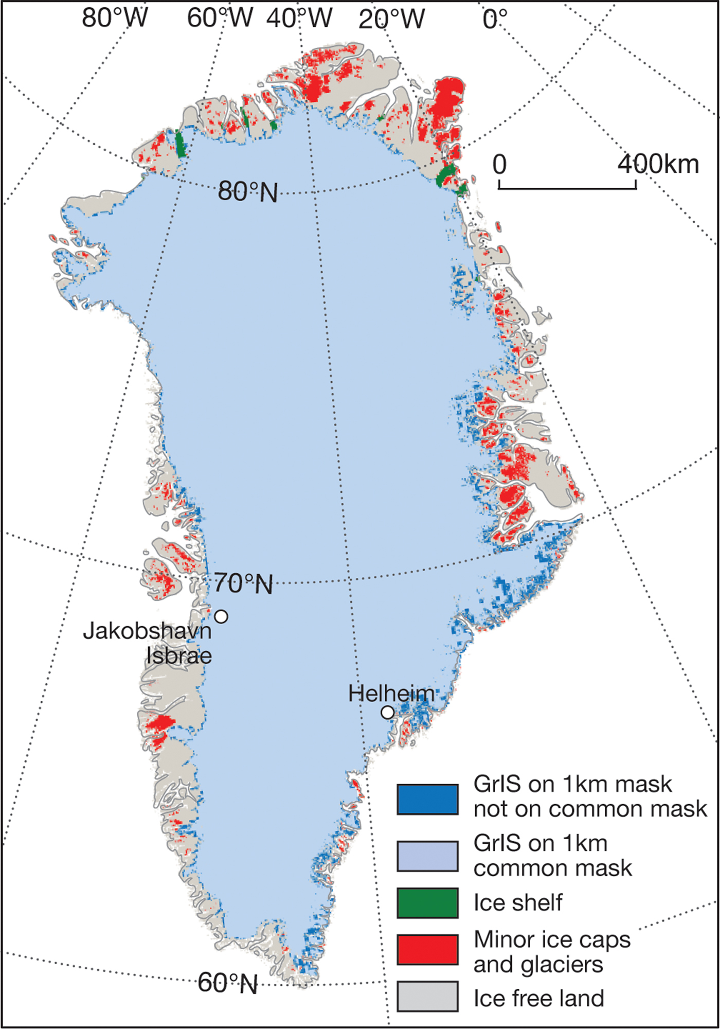
Fig. 1. Greenland ice mask on the 1 km × 1 km spatial resolution grid adapted from that of Bamber and others (Reference Bamber2013). The full 1 km ice mask as used for our PDD models comprises the areas covered by the two blue colours. The light blue colour corresponds to the common ice mask for the PDD model and the two RCMs compared in Section 3.1.2.
The paper is structured as follows. Section 2 describes the key datasets and methods underpinning this work. Section 3 presents the results in three parts: Section 3.1 has results for the whole GrIS compared with both previous work at 5 km (3.1.1) and with state-of-the-science regional climate models (RCMs) on a common ice mask (3.1.2). Section 3.2 discusses SMB changes at the drainage-basin scale, while Section 3.3 focuses on much more local runoff changes around key calving glaciers and briefly compares these with glacier dynamic changes. Section 4 provides a synthesis of our key findings.
2. DATA AND METHODS
2.1. Climate and meteorological data
Monthly near-surface air temperature, precipitation, sublimation and evaporation, derived from the latent heat flux, were obtained from 20CR (1870–2010) and ERA-I (1979–2012), and bi-linearly interpolated from 2° × 2° and 0.75° × 0.75° respectively, to a 1 km × 1 km polar stereographic grid (Bamber and others, Reference Bamber2013). For our full time series 20CR was used from 1870 to 1979 and ERA-I from 1980 to 2012, the runoff algorithm requiring a 1-year spin-up period. The data from the two reanalyses were spliced together as described in Hanna and others (Reference Hanna2011) to prevent any discontinuity. Temperatures were corrected for differences between the reanalysis orography, interpolated to the 1 km grid, and a reference DEM on the 1 km grid (Bamber and others, Reference Bamber2013) using empirically derived near-surface air temperature lapse rates (−6 to −8°C km−1), following Hanna and others (Reference Hanna2005, Reference Hanna2011). All 20CR temperatures were also further scaled so that for the overlap period of 1979–2010 averages for each month matched those of ERA-I. Precipitation was spatially calibrated against the Bales and others (Reference Bales2009) kriged corrected precipitation map, interpolated to the 1 km grid. The 20CR data were then rescaled so that each month's data had the same variance as ERA-I (for the overlap years). Evaporation or sublimation data were obtained from the reanalysis latent heat flux by dividing by the appropriate latent heat of vaporization (2.50 × 10⁶ J kg−1) or sublimation (2.83 × 10⁶ J kg−1), with the monthly average temperature being used to discriminate between both: i.e. if temperature is above 0°C then evaporation is calculated, whereas if temperature is below 0°C sublimation is assumed. As sublimation likely dominates over the GrIS (ERA-I mean annual (mean summer, JJA) 2 m air temperature = −20.1 (−7.0)°C), for brevity we hereafter use the term sublimation to refer to both evaporation and sublimation. Again for 20CR this is scaled so that its mean matches that of the ERA-I – the latter being deemed more realistic (Hanna and others, Reference Hanna2011) – for the overlap years. This had the effect of scaling 20CR sublimation by a factor of 0.3.
The Bamber and others (Reference Bamber2013) surface DEM is based on the 2000–09 period. Before the 1990s the ice-sheet mass balance was relatively steady compared with the recent period of strong Arctic warming (e.g. Rignot and others, Reference Rignot, Box, Burgess and Hanna2008). However, there has only been an estimated ~0.8% reduction in the ice sheet's area, or ~363 m mean horizontal retreat of its margin, since 1900 (Beitch, Reference Beitch2014). Elevation changes arising from net mass-balance changes are <1 m a−1 for most of the ice sheet and are only really prominent in the immediate vicinity of major outlet glaciers (Kjeldsen and others, Reference Kjeldsen2015, their Fig. 2a). Given the 1 km × 1 km spatial resolution of our SMB model output, this is not expected to seriously affect our results regarding ice sheet SMB values and trends since 1870.
2.2. Ice mask
An ice mask, on the same 1 km grid is used, which indicates whether a pixel is part of the GrIS, as shown in Figure 1. The other categories, for which we do not calculate SMB, are ice-free land, ocean, ice shelf or other ice not part of the GrIS, such as smaller ice caps and isolated glaciers. The ice mask used is essentially that of Bamber and others (Reference Bamber2013) but with our own modification to define non-GrIS minor ice caps and glaciers (MICG). This was achieved as follows. Initially we classed all grounded ice pixels as MICG. Next a group of pixels that were clearly GrIS, in the centre of Greenland, were manually classed as GrIS. We then examined all remaining pixels classed as MICG and changed their class to GrIS if they were in contact with an existing GrIS pixel. This step was then repeated until the number of GrIS pixels remained constant for successive iterations. This ultimately left as MICG only those pixels not in contact with the main GrIS, as shown in Figure 1. This gives a total area for the GrIS of 1730643 km2. The 5 km resolution ice mask used in Hanna and others (Reference Hanna2011) had a 3% smaller GrIS area, which should be borne in mind when comparing results. Differences in ice masks used can lead to some of the difference in results from different methods of calculation, as discussed by Vernon and others (Reference Vernon2013), and ideally we would want to compare results for the same ice mask. However, because one of our main sources of difference from Hanna and others (Reference Hanna2011) is the use of a much higher resolution ice mask, some difference in the total area of the GrIS is inevitable. In Section 3.1.2 where we compare with RCMs, we do use a common ice mask, as shown in Figure 1, so that our results are for the exact same definition of GrIS.
2.3. PDD modelled SMB
SMB is defined as precipitation minus sublimation minus runoff. The first two terms in that equation are obtained from the calibrated/corrected reanalysis data as described above. Runoff is calculated from the PDD runoff/retention model of Janssens and Huybrechts (Reference Janssens and Huybrechts2000), where retention is based on re-freezing and capillary forces in the snowpack (Pfeffer and others, Reference Pfeffer, Meier and Illangasekare1991), summarized in Hanna and others (Reference Hanna2005, Reference Hanna2011). Standard PDD factors for the GrIS of 7.2 (2.7) mm w.e. d−1 °C−1 for ice (snow) are adopted from Janssens and Huybrechts (Reference Janssens and Huybrechts2000), and although it is recognised that these can vary over space and time (e.g. Braithwaite, Reference Braithwaite1995) there are few reliable data to constrain them for the whole ice sheet since 1870. Ice PDD factors for Greenland presented in Hock (Reference Hock2003) suggest no systematic change between ~1950 and 2000. There are no such data available before 1950 and only three before 1980, however the available evidence does therefore suggest that long-term changes in PDD factors will not significantly affect our SMB model results. Also, although it is a source of uncertainty, the use of fixed PDD factors is in line with other long-term PDD-based GrIS SMB model results recently reported (e.g. Hanna and others, Reference Hanna2011, Box and others, Reference Box2013). The number of PDDs is calculated from monthly air temperature and monthly standard deviation or sigma (σ) of the daily or sub-daily near-surface air temperature, and is a standard method used in this type of model. Sigma accounts for temperature variations arising from the diurnal cycle and random weather fluctuations. In the original model a constant value of σ = 4.2°C was assumed (Reeh, Reference Reeh1991; Janssens and Huybrechts, Reference Janssens and Huybrechts2000), as used in Hanna and others (Reference Hanna2011). In the present work we use variable σ calculated from the downscaled 20CR or ERA-I 3- or 6-hourly 2 m air temperatures across the GrIS on the 5 km resolution grid, as described in Jowett and others (Reference Jowett, Hanna, Ng, Huybrechts and Janssens2015). The 20CR and ERA-I data were spliced together and interpolated to the 5 km gird, in the same way as described here in Section 2.1. Monthly σ for each point on that grid was then calculated as the standard deviation of the 3- or 6-hourly values for that month. This produces a spatially varying σ value for every month of the study period (1870–2012 inclusive). Across this time period σ varies primarily depending upon elevation and season. The mean annual distribution shows that lower σ values (as low as 1°C) dominate around the periphery of the ice sheet. The value of σ then increases towards the centre of the ice sheet up to ~9°C at the highest elevations. Values of 4–6°C cover the majority of the ice sheet. During the summer however, the spatial distribution is very different, with 1–2°C values penetrating further inland. The highest values are again in the centre of the ice sheet but only reach up to 5–6°C. Full details of this modification are reported in Jowett and others (Reference Jowett, Hanna, Ng, Huybrechts and Janssens2015), and this also follows recent similar work by Rogozhina and Rau (Reference Rogozhina and Rau2014). It is assumed that σ for a pixel on the 1 km grid is the same as that for the 5 km pixel containing it, time and storage requirements prohibiting this calculation on the 1 km grid.
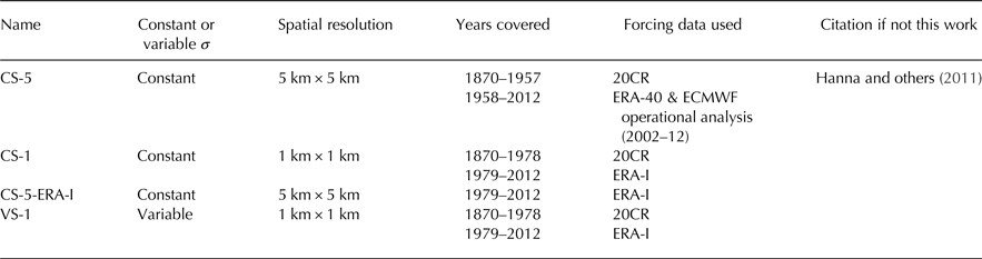
Our runoff and SMB time series, hereafter VS-1, represent an advance on those of Hanna and others (Reference Hanna2011) in that the spatial resolution is increased from 5 km × 5 km to 1 km × 1 km, and variable, rather than assumed constant, σ are used. We employ a considerably longer timescale and finer spatial resolution than Rogozhina and Rau (Reference Rogozhina and Rau2014), who based their analysis on an older (ERA-40) version of the ECMWF reanalysis. We also include results on the 1 km grid using constant σ = 4.2°C, hereafter CS-1, so that differences due to the grid resolution alone can be assessed. Table 1 summarizes the different PDD results presented here and abbreviations used hereafter.
Table 1. Summary of different PDD models included in this work and those with which we compare
As well as calculating runoff and SMB for the entire GrIS we also examine these at more local scales. We divide the ice sheet into seven drainage basins, following Barletta and others (Reference Barletta, Sorensen and Forsberg2013), and secondly focus on the areas around two specific glaciers, Helheim Glacier in the southeast, and Jakobshavn Isbræ in the west.
2.4. SMB from RCMs
In order to assess our VS-1 model results we also compare with the output of two RCMs: the Modèle Atmosphérique Régional (MAR version 3.5.2) (Fettweis and others, Reference Fettweis2013) and the Regional Atmospheric Climate MOdel (RACMO2.1) (Van Angelen and others, Reference Van Angelen, van den Broeke, Wouters and Lenaerts2014). Both models are fully coupled with energy and mass balance-based snow models taking into account the surface atmosphere feedbacks and are forced at their lateral boundaries (around the GrIS) by ERA-40 reanalysis data over 1958–78 and ERA-I afterwards. They were run at a spatial resolution of ~11 km (RACMO) and 10 km (MAR), respectively. Both of them explicitly simulate all the SMB components and their ability to model GrIS SMB has previously been demonstrated by Ettema and others (Reference Ettema2009); Fettweis and others (Reference Fettweis, Tedesco, van den Broeke and Ettema2011) and Van Angelen and others (Reference Van Angelen, van den Broeke, Wouters and Lenaerts2014). We refer the reader to these papers for a more detailed description of both RCMs.
3. RESULTS AND DISCUSSION
3.1. Total GrIS runoff and SMB
Figure 2 shows the annual GrIS SMB (VS-1) and its components calculated by the PDD method as described in Section 2.3; sublimation is included in this Figure for completeness but makes a negligible contribution to trends in SMB. In the following discussion the quoted values refer to the ±5 year moving averages. Up to 1925 annual precipitation gradually increases to 773 Gt a−1, while annual runoff gradually decreases to 123 Gt a−1 and sublimation remains relatively constant with a value of 65 Gt a−1 in 1925. This therefore leads to an overall increase in annual SMB to a peak of 586 Gt a−1 in 1925. Between 1925 and 1995 precipitation decreases to 618 Gt a−1, runoff remains relatively stable, following a short period of increase ~1930, reaching 216 Gt a−1 with sublimation again relatively stable, after an initial drop, at 46 Gt a−1 by 1995. These trends thereby result in SMB falling over the mid to late 20th century reaching 356 Gt a−1. From 1995 onwards runoff increases rapidly to 404 Gt a−1 by 2007, while precipitation increases slightly to 637 Gt a−1 in 2003 before decreasing to 619 Gt a−1 in 2007 and sublimation remains ~46 Gt a−1. This leads to a corresponding sharp decrease in SMB after 2000, to 170 Gt a−1 by 2012.
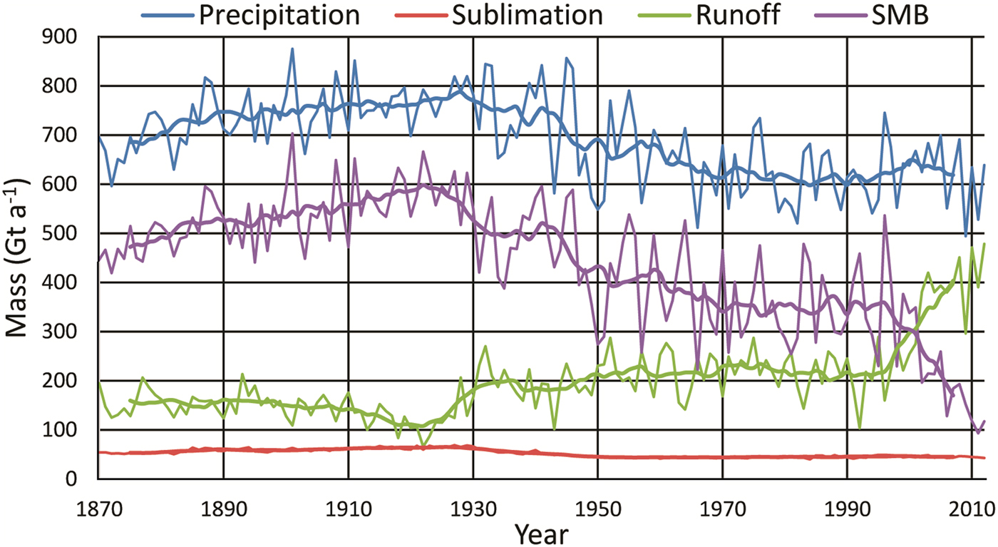
Fig. 2. Annual GrIS SMB (VS-1) and component parts (precipitation, runoff and sublimation). Thin lines show the actual annual values and the thick lines show ±5 year moving averages.
3.1.1. Comparison with previous PDD results
Similar trends for SMB and its component parts were noted by Hanna and others (Reference Hanna2011), using a PDD model at 5 km resolution (CS-5), but our present results show a much sharper rise in runoff from 2000 onwards. Figure 3 shows a direct comparison of our present precipitation, runoff and SMB, VS-1 and CS-1, results with the 5 km (CS-5) from Hanna and others (Reference Hanna2011). We include CS-1 results, i.e. those calculated with constant σ, as this was the parameterization used by Hanna and others (Reference Hanna2011) and so allows us to compare the effects of the higher spatial resolution and variable σ separately. We also show new CS-5-ERA-I results, i.e. 5 km × 5 km resolution with constant σ calculated with ERA-I data to demonstrate any effects due to the different reanalysis data used. The VS-1 annual runoff, blue line in Figure 3b, is consistently lower than CS-5, green line, up to the early 2000s when a much steeper increase in the VS-1 runoff leads to it becoming larger than CS-5 (the opposite is obviously the case for SMB). The reason for this difference involves multiple factors. Comparing CS-1 with CS-5 runoff shows the effect of different resolution grids alone. CS-1 runoff is almost always higher than CS-5 because the 1 km grid covers more low-lying area having a higher temperature. For example the total area under 250 m elevation is 14 788 km2 for the 1 km grid and 10 350 km2 for the 5 km grid. The only exception occurs from 1979 onwards when CS-1 is using ERA-I and CS-5 ERA-40 (and ECMWF operational analysis) data. From 1870 to 1958, when CS-1 and CS-5 results are using the same 20CR data, the difference is a fairly consistent, ~43 Gt a−1; only in the late 1920s and early 1930s does the gap narrow noticeably when the rise in CS-1 is slightly steeper than that in CS-5. Similarly, if we compare CS-1 post 1979 with CS-5-ERA-I, we again see that the former is always greater than the latter with a mean annual difference of 58 Gt a−1. Therefore, in line with previous work (Reeh and Starzer, Reference Reeh and Starzer1996), increasing the spatial resolution alone increases runoff and thus decreases SMB. Over 1870–2012 CS-1 annual runoff is greater than VS-1 by an average of 74 Gt a−1. Figure 3a shows that the 1 km resolution models have consistently greater total precipitation than the 5 km with the same forcing data, i.e. up to the mid-1950s. This can only be due to different areas covered by the respective ice masks as both simply involve the statistical downscaling and recalibration of the reanalysis data on the appropriate higher resolution grid: i.e. the 3% lesser area of the 5 km mask leads to ~50 Gt a−1 less annual precipitation than the 1 km mask. Interestingly this lower precipitation for the 5 km models is cancelled out by the sum of a similarly lower runoff and sublimation (not shown) so that the SMB for CS-1 and CS-5 are almost identical for the period where they use the same 20CR forcing.
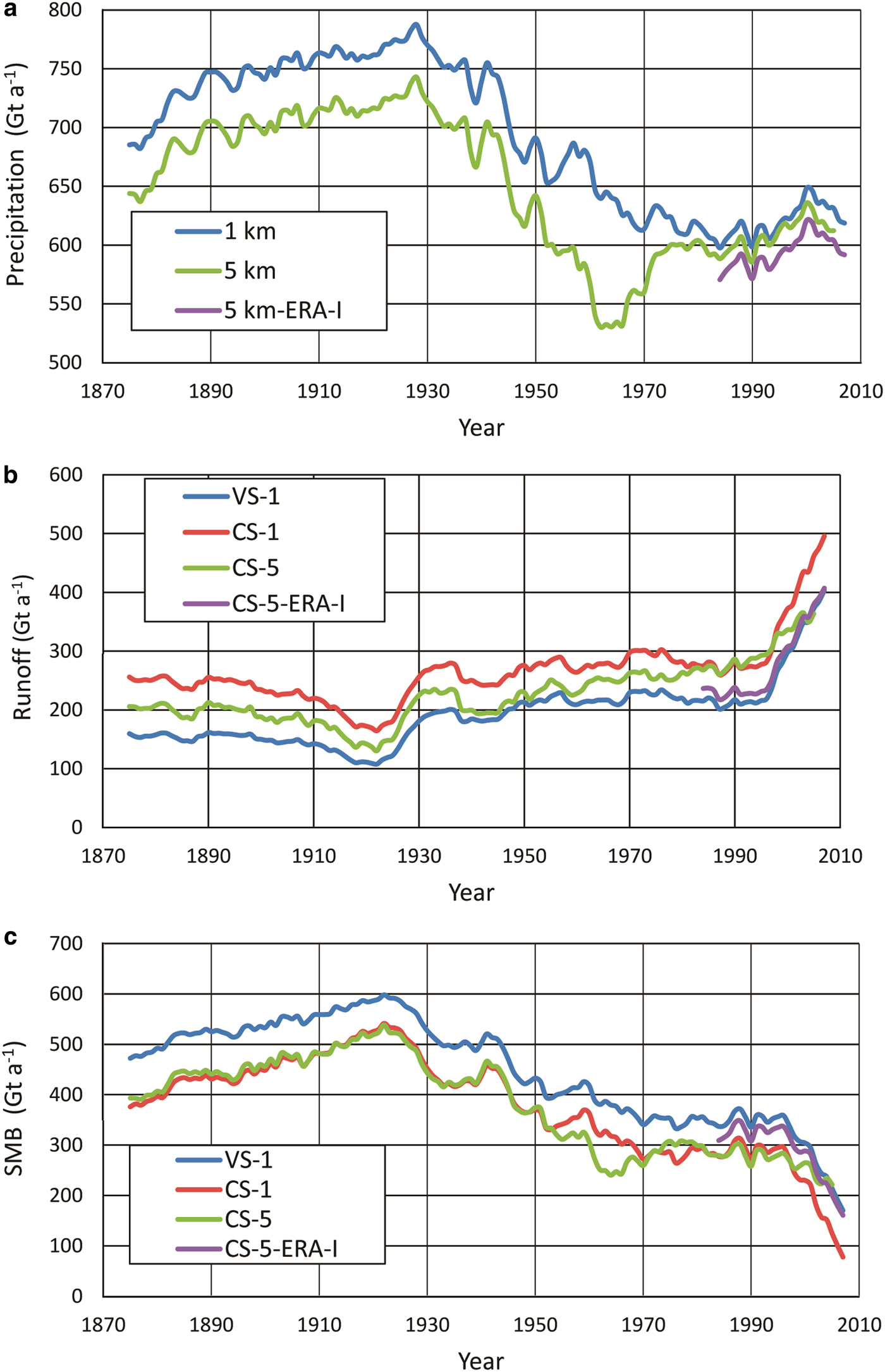
Fig. 3. The ±5 year moving averages of (a) precipitation, (b) runoff and (c) SMB, showing comparison of 1 km and 5 km spatial resolution. Models are as described in Table 1. For precipitation the values shown are simply downscaled re-analysis data that have been spatially calibrated against the in situ-based Bales and others (Reference Bales2009) Greenland accumulation map, as described in the main text Section 2.1. 1 km is that used with CS-1 and VS-1, 5 km is that used with CS-5 and 5 km-ERA-I is that used with CS-5-ERA-I.
The effect of changing from constant to variable σ alone is shown by the comparison of CS-1 and VS-I for runoff in Figure 3b. In agreement with the conclusions of Jowett and others (Reference Jowett, Hanna, Ng, Huybrechts and Janssens2015) and Rogozhina and Rau (Reference Rogozhina and Rau2014) we find that VS-1 gives consistently lower runoff and higher SMB than CS-1. This corresponds to fewer PDDs through less variable temperatures, therefore fewer relatively high temperature extremes and consequently, reduced melting and runoff in the ablation zone of the ice sheet.
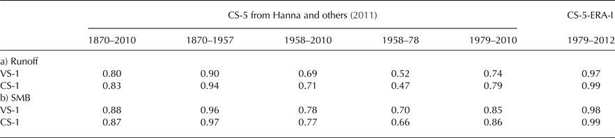
The 1 km runoff and SMB can be seen to be highly correlated with their 5 km equivalents, r = 0.80 and 0.88 respectively, for detrended data, but that correlation is clearly worse from ~1960 onwards. Table 2 shows an analysis of correlations over periods depending on the data used here and in Hanna and others (Reference Hanna2011). All correlations shown are statistically significant at the 95%, or higher, confidence level. However the correlation coefficients are clearly, and unsurprisingly, highest for the period 1870–1957 where both 1 km and 5 km results use the same 20CR data and lowest for 1958–78 where the 1 km use 20CR but the 5 km use ERA-40. The correlations are even higher for 1979–2012 if we compare with 5 km using just ERA-I data. Therefore the change in qualitative agreement between the 1 km and 5 km results post 1960 appears to be due to the difference in forcing data used.
Table 2. Correlation between 1 km and 5 km runoff or SMB. Pearson's correlation coefficient with de-trended data. The 1 km resolution results (this work) and 5 km equivalents are shown for different ranges of overlapping years. The data used vary over time. For 1870–1957 both use 20CR. For 1958–78 this work uses 20CR whereas Hanna and others (Reference Hanna2011) use ERA-40. For 1979–2008 this work uses ERA-I whereas Hanna and others (Reference Hanna2011) use ERA-40 plus ECMWF operational analysis data. Additional comparison is made between our 1 km results and 5 km (CS) using ERA-I data. The 1 km dataset is either the principal version with runoff code using actual standard deviations of temperature (VS) or that with assumed constant value of standard deviations of temperature (CS). The 5 km results all use the latter
As discussed earlier, just changing from the 5 km to 1 km resolution grid increases runoff, as shown in Figure 3b when considering the 1 km (CS) results in relation to either set of 5 km (CS) results. Plots of the average annual runoff for the period 1990–2010, zoomed into two specific areas of Greenland, for our 1 km (CS) and Hanna and others (Reference Hanna2011) 5 km (CS) resolution results are shown in Figure 4. It shows the far southern tip of the GrIS, ~61°N 44°W, and the mid west area ~72°N 52°W. The ability of the 1 km grid to show individual glaciers that are below the resolution of the 5 km grid is clear in these examples. These glaciers, at lower elevation, and therefore higher temperature than the surrounding ice sheet, will have higher rates of runoff. The 1 km grid can resolve these whereas for the 5 km those glaciers will be averaged into a 5 km× 5 km pixel, which will tend to have a higher elevation and hence a lower runoff from the ice sheet. This can be clearly seen by the deeper red coloured, i.e. higher runoff, pixels on Figures 4a, c as compared with equivalent places on Figures 4b, d. For example this is particularly notable in Figure 4c where we can clearly see three well-resolved, high-runoff, glaciers in the centre of the figure whereas in Figure 4d the same glaciers are poorly resolved and have lower runoff. It is also clear that there are some areas defined as GrIS on the 1 km grid ice mask that are not on the 5 km, as can be seen by lobes of ice sheet in Figure 4a on the east of the ice sheet that are clearly not present on Figure 4b. However, while these additional areas of ice sheet will have the potential to raise the overall runoff significantly for the 1 km results, it can again be seen that it is only on the edges of the ice sheet, where the 1 km grid is able to resolve much finer detail, that additional runoff is found. It is therefore the enhanced level of detail in the 1 km grid that must be the factor leading to the difference that changing the resolution alone produces.
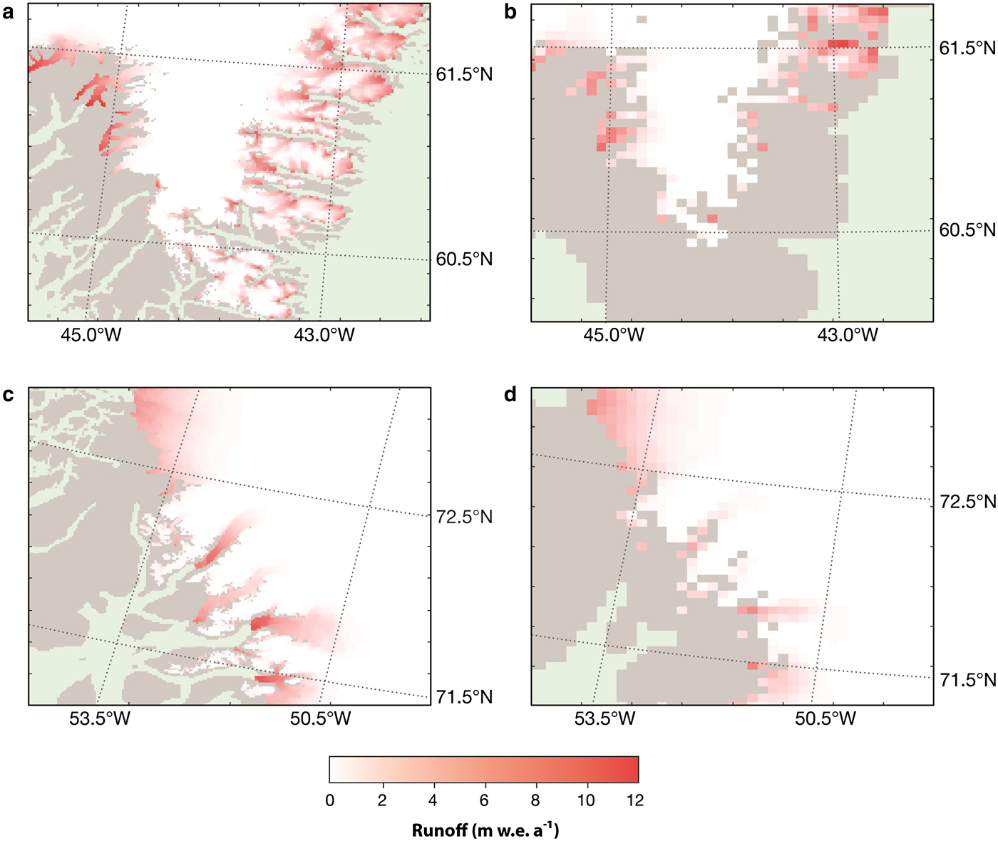
Fig. 4. Mean annual runoff 1990–2010, for specific parts of the south of the GrIS, (a) CS-1 and (b) CS-5, and the mid west of the GrIS, (c) CS-1 and (d) CS-5. Abbreviations as described in Table 1. Grey areas are ice-free land and green areas ocean.
3.1.2. Comparison with RCM results for whole ice sheet SMB and in situ observations
We now compare the VS-1 results with those from the RCMs, MARv3.5.2 and RACMO2.1, as described in Section 2.4, from 1979 to 2012, the period for which all three models have the same ERA-I forcing. Note that the purpose here is to evaluate VS-1 in the context of RCM results, rather than assess the two RCMs, which undergo frequent updates. The RCMs have significantly different ice masks to the 1 km mask we have used for our PDD results. Therefore in order to eliminate differences in ice mask as the potential cause of difference in results, we have derived a common ice mask that is used for all results discussed in this section. This is shown in Figure 1. It was achieved by interpolating the RCM ice masks to the 1 km grid and then keeping as GrIS only those pixels classed as GrIS for all three masks.
Figure 5 shows the annual total GrIS precipitation, runoff and SMB and Figure 6 shows the mean for 1979–2012 of these three variables over the whole common mask GrIS for VS-1, RACMO2.1 and MARv3.5.2. The precipitation used for VS-1 is always lower than that from either RCM but is highly correlated with them: the detrended correlation coefficient r for PDD vs MARv3.5.2 is 0.95 and for PDD vs RACMO2.1 is 0.94, both statistically significant at the 99% confidence level. We would expect a difference in precipitation since that used for the PDD model is statistically downscaled reanalysis data (calibrated against a map derived from in situ data interpolated to the 1 km grid) whereas for the others it is from a RCM, i.e. dynamically downscaled, in line with previous results in Vernon and others (Reference Vernon2013). There remains considerable uncertainty over what is the ‘real’ mean precipitation over Greenland, due to lack of adequate in situ validation data, especially in southeast Greenland (Bales and others, Reference Bales2009; Hanna and others, Reference Hanna2011; Box and others, Reference Box2013). Ettema and others (Reference Ettema2009) hypothesized that the inherently high spatial resolution of the RACMO2.1 RCM may simulate high-intensity precipitation in the southeast coastal mountains more realistically than previous model simulations. GrIS annual total runoff for VS-1 is also in agreement with the RCMs, Figure 5b: de-trended r for PDD vs MARv3.5.2 is 0.78 and for PDD vs RACMO2.1 is 0.77, again both significant at the 99% confidence level. VS-1 gives the lowest annual runoff and RACMO2.1 the highest. Figure 5c shows that SMB for the VS-1 is quite similar to that from both RCMs. The respective annual means of SMB from 1979 to 2012 are 382, 379 and 425 Gt a−1 respectively, for VS-1, RACMO2.1 and MARv3.5.2. Again the values of de-trended r also show high correlations between VS-1 and both RCMs: 0.87 for MARv3.5.2 and 0.89 for RACMO2.1. The gradients of the linear trends for SMB and its main constituent parts for the three models, Table 3, do show some differences. The negative trend in SMB is lower for VS-1 (−3.65 Gt a−2) than for either of the two RCMs (−5.74 and −5.34 Gt a−2 for RACMO2.1 and MARv3.5.2 respectively), mainly due to a lower positive trend in runoff. If we just consider the last 15 years all models show a much more negative SMB trend: −11.38 Gt a−2 for VS-1 compared with −14.01 and −15.44 Gt a−2 for the RCMs. However, none of the differences in any pairs of gradient are statistically significant. Given the standard errors, also shown in Table 3, the probabilities that the gradients of two different models for the same variable are significantly different are all <0.05. It is clear from Figure 5c that the most significant change in SMB has occurred in the last 10–12 years. Prior to that SMB fluctuated significantly for some years but remained relatively stable on average. However, from 2000 to 2012 all three models agree that there has been a significant and sustained decrease.
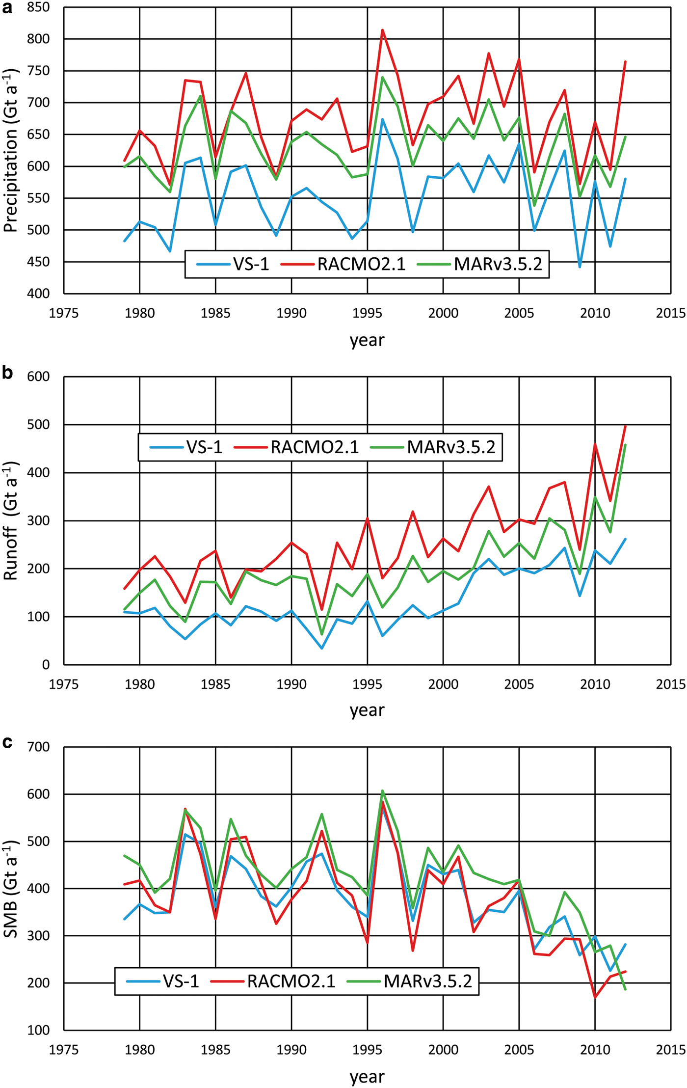
Fig. 5. Annual GrIS (a) precipitation, (b) runoff and (c) and SMB for VS-1 compared with RACMO2.1 (Van Angelen and others, Reference Van Angelen, van den Broeke, Wouters and Lenaerts2014) and MARv3.5.2 (Fettweis and others, Reference Fettweis2013), 1979–2012.
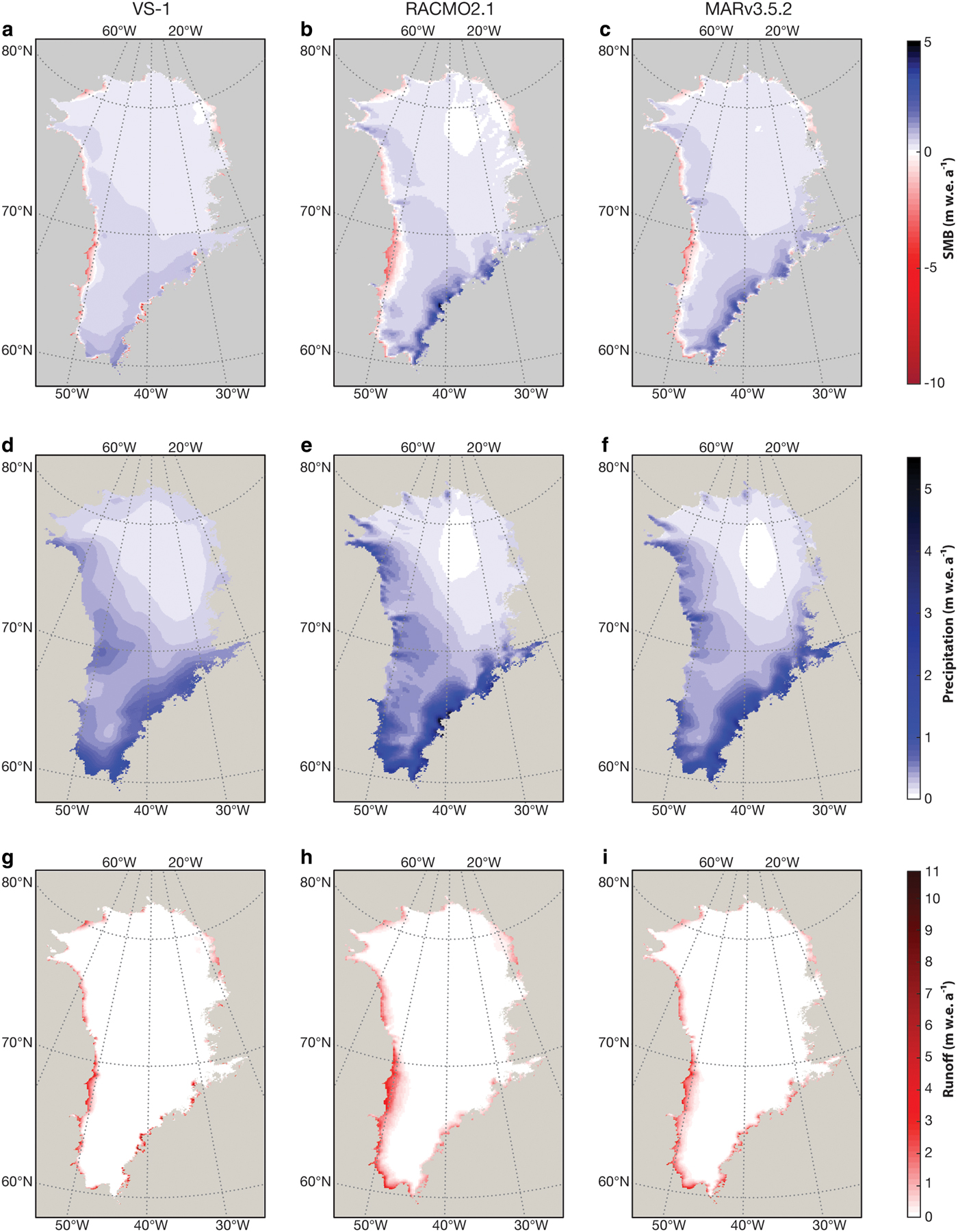
Fig. 6. Mean GrIS 1979–2012 SMB for (a) VS-1, (b) RACMO2.1 (Van Angelen and others, Reference Van Angelen, van den Broeke, Wouters and Lenaerts2014) and (c) MARv3.5.2 (Fettweis and others, Reference Fettweis2013) on 1 km ice mask common to all three models. Similar means for each model's precipitation (d) VS-1, (e) RACMO2.1 and (f) MARv3.5.2, and runoff (g) VS-1, (h) RACMO2.1 and (i) MARv3.5.2.
Table 3. Gradients (Gt a−2) of linear fits to precipitation, runoff and SMB. Standard errors are given in brackets. VS-1 compared with RACMO2.1 (Van Angelen and others, Reference Van Angelen, van den Broeke, Wouters and Lenaerts2014) and MAR version 3.5.2 (Fettweis and others, Reference Fettweis2013), for 1979–2012 and 1998–2012, calculated on a common ice mask
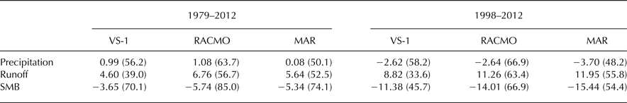
Figure 6 shows the mean 1979–2012 SMB, precipitation and runoff at each point on the 1 km common grid for VS-1, RACMO2.1 and MARv3.5.2. We can see that in the west, north and northeast of the GrIS the three models are in good agreement. The SMB is generally a small positive value over these regions, other than at the edges where all three models show clear regions of negative SMB stretching many kilometres inwards. The extent of the negative SMB region in the mid west and southwest is clearly greatest for RACMO2.1 and least for VS-1. In the southeast of the GrIS all three models agree that SMB is significantly positive away from the very eastern edges, but that the magnitude of the positive SMB region is clearly greater for the RCMs than for VS-1. We can also see clear areas of positive SMB on the eastern edges of the southeast part of the GrIS for VS-1 and MARv3.5.2 but not for RACMO2.1. The greater positive SMB for the RCMs compared with VS-1 in the southeast will be due to the greater precipitation for the RCMs, clear from Figures 7d–f, and this region of the GrIS is known to experience the highest rates of precipitation (Bales and others, Reference Bales2009). The clearly more negative SMB in the mid west and southwest for the RCMs can be attributed to their greater runoff (Fig. 6g–i), as this part of the GrIS has experienced strong warming in recent years (Hanna and others, Reference Hanna, Mernild, Cappelen and Steffen2012, Reference Hanna2014). As we have noted that overall VS-1 and the RCMs give similar SMB over 1979–2012, it must be the case that the more positive SMB the RCMs show in the southeast is cancelled out by the more negative SMB in the mid to southwest when we sum over the whole ice sheet.
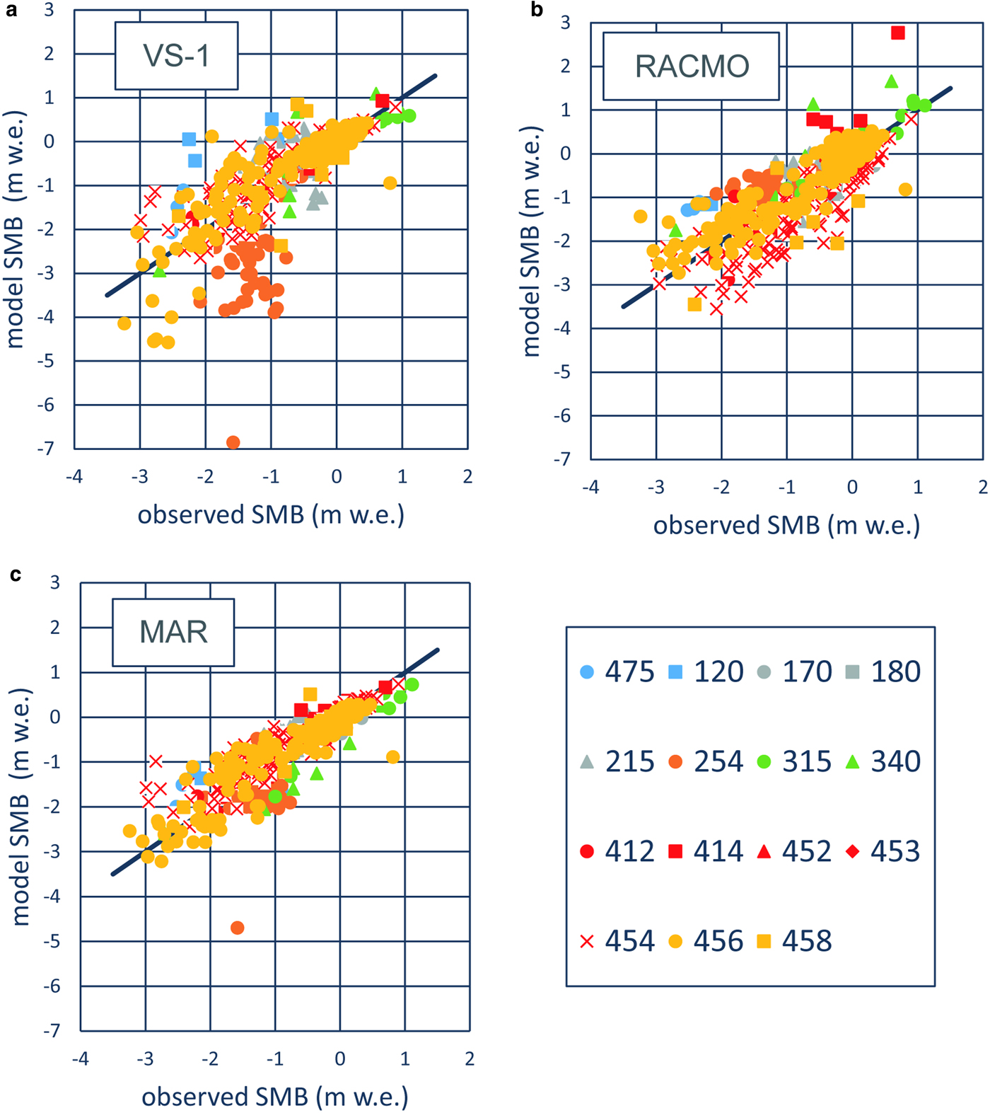
Fig. 7. Scatter plots of model vs measured SMB for PROMICE observations at sites on the common ice mask, (a) VS-1, (b) RACMO2.1 (Van Angelen and others, Reference Van Angelen, van den Broeke, Wouters and Lenaerts2014), (c) MARv3.5.2 (Fettweis and others, Reference Fettweis2013). Each glacier is indicated by a specific marker colour – shape combination given in the legend by their PROMICE glacier numbers. The colour of the markers indicates the region of the GrIS: blue is northwest, grey northeast, brown southeast, green south, red southwest and yellow mid west. The solid black line corresponds to model = observed.
We also assess the VS-1 and RCM results with respect to observations. The Programe for the Monitoring of the Greenland ice sheet (PROMICE), (Machguth and others, Reference Machguth2016) is a data base of SMB measurements in the ablation zone of the GrIS and other local glaciers. It includes sites from 18 different glaciers or areas that have observations starting and finishing on dates between January 1979 and December 2012 and that are within the GrIS as defined by our full 1 km ice mask. Each site then has observations at multiple locations, many of which are not within our ice mask, and multiple dates. Of the original 2947 observations between 1979 and 2012 there are 1158 classed as GrIS, of which 929 are on the full 1 km ice mask and 467 on the common ice mask. The latter is the total number of observations with which we can assess and intercompare the model results. These are summarized in Table 4. We compare each PROMICE observations with that for the model pixel closest to it and starting and finishing at approximately the same dates; the models all run on a monthly time step whereas the observations are given as calendar dates. As VS-1 is run at 1 km resolution the model SMB values will usually be from a point closer to the observations than those of the RCMs run at ~10 km resolution. Model SMB is taken as the sum of monthly values for the whole months the observations are taken over, plus the appropriate fractions of the start and end months. Figure 7 shows scatter plots for each model against the PROMICE observations. The scatter plots are colour coded by the region of the GrIS they come from and different marker shapes indicate different glaciers. For the three models Pearson's correlation coefficient, r, and RMSE are shown in Table 5. This demonstrates that when considering all observations the PDD method does not match them as well as more sophisticated RCMs, having higher error and lower, but still clearly positive, correlation. As Figure 7a shows there are more outliers for the VS-1 model than for either of the RCMs. Two glaciers stand out as clear outliers for VS-1, 254 (Helheim) in the southeast and 475 (Tuto Ramp) in the northwest, although there are only three observations for the latter. In both cases this is almost certainly due to the lower values of precipitation leading to lower SMB for VS-1 in the southeast and, to a lesser extent, northwest, as discussed previously.
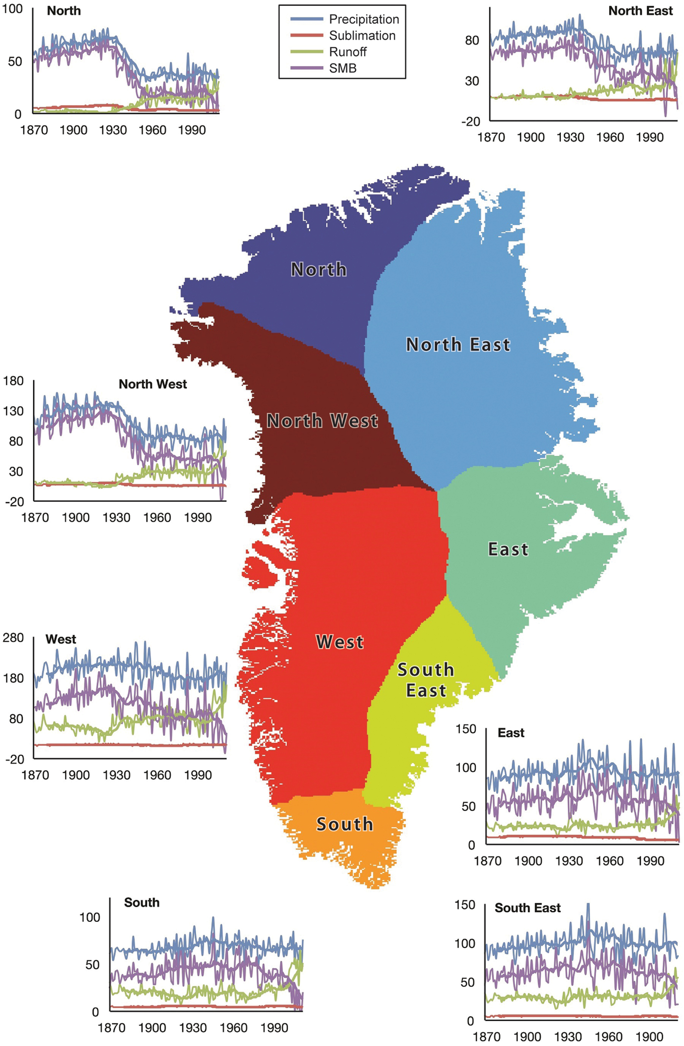
Fig. 8. The 1 km resolution SMB, in Gt a−1, and component parts for seven drainage basins of GrIS (Barletta and others, Reference Barletta, Sorensen and Forsberg2013).
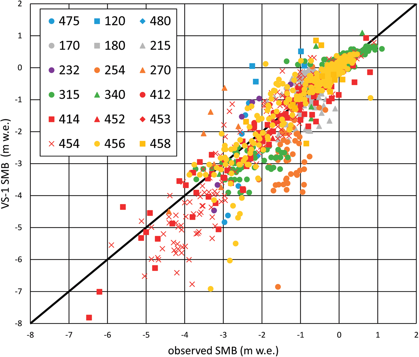
Fig. 9. Scatter plot of VS-1 model vs measured SMB for PROMICE observations at sites on the full 1 km ice mask. Each glacier is indicated by a specific marker colour – shape combination given in the legend by their PROMICE glacier numbers. The colour of the markers indicates the region of the GrIS: blue is northwest, grey northeast, brown southeast, green south, red southwest and yellow mid west. The solid black line corresponds to model = observed.
Table 4. Summary of PROMICE GrIS SMB observations with which model results are compared
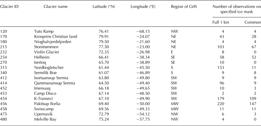
The number of observations refers to those both within the time span (1979–2012) during which the VS-1 and RCMs models overlap and within the GrIS as defined by the full 1 km ice mask and the common ice mask. Glacier ID is that used in Machguth and others (Reference Machguth2016). The region of GrIS is essentially the same as the drainage basins shown in Figure 8 other than that for clarity on the scatter plots (Figs 7, 9) we split the glaciers from the west basin into south west and mid west.
Table 5. RMSE and Pearson's correlation coefficient of model vs measured SMB for PROMICE observations at sites on the common ice mask
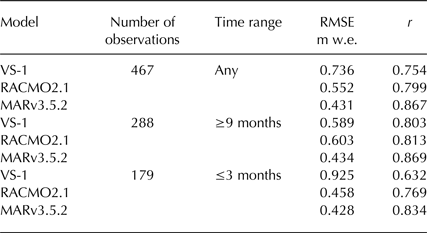
The observations are not all taken over the same amount of time. Almost all of them can be split into one of two groups in terms of their start and end dates. Around 56% of the sites have an August or September start date and an end date in May–September the following year. These observations correspond to around a year and include most or all of that year's melt. Another ~36% of the observations start in May–July and finish in the same year's July–August. These therefore correspond to a couple of months in the melt season only. The remainder either have observations over more than 2 years or less than a whole month. We can split the observations into two sets and calculate correlation separately. As shown in Table 5, for all models correlations are poorer with respect to those observations over just a couple of months. This includes all but one of the observations at Helheim glacier. But with respect to observations over at least 9 months VS-1 has r and RMSE close to that of RACMO2.1 while that for MARv3.5.2 remains clearly the highest. This therefore gives us confidence that at least with respect to annual SMB values the PDD method is broadly comparable, though not quite as good, as the RCMs.
3.2. Drainage basin scale runoff and SMB
Plots of annual SMB, precipitation, runoff and sublimation for seven Greenland drainage basins (Barletta and others, Reference Barletta, Sorensen and Forsberg2013) are shown in Figure 8. Again, sublimation is shown for completeness but makes only small contributions to trends in SMB. As some basins show very similar trends, they are discussed in four groups as follows.
3.2.1. The north, northeast and northwest basins
These show very low values of annual runoff of <10 Gt a−1 up to ~1930, which then increases to 30 Gt a−1 before rising sharply after 2000, to peak values of 20–60 Gt a−1 dependent upon the specific basin. Relatively low runoff is to be expected here due to the high latitude resulting in lower temperatures. Precipitation rises gently from 1870 to 1930, to an annual peak of ~80–100 Gt a−1 or more depending upon the basin, then drops more steeply until 1960 after which it levels out ~30–50 Gt a−1 lower than the peak value. The reason for the change in precipitation ~1930 is unknown but could be related to a warm peak in Greenland around the same period (Box and others, Reference Box, Yang, Bromwich and Bai2009; Hanna and others, Reference Hanna, Mernild, Cappelen and Steffen2012). The SMB for these basins is therefore influenced almost entirely by precipitation before 1930, being ~10–20 Gt a−1 lower than the corresponding value of precipitation, and thereafter becomes more influenced by runoff with SMB values of 20–50 Gt a−1 up to 2000. We see a sharp drop in SMB from 2000 onwards with some years even having negative SMB.
3.2.2. The east and southeast basins
These areas both show fairly low runoff, 20–30 Gt a−1, with small interannual variability and then a sharp increase from 2000 onwards to peak values of 40–50 Gt a−1. Precipitation gradually rises from 1870 to the 1940s, to peaks ~120 Gt a−1, before decreasing and levelling out at 90–100 Gt a−1 from ~1970 onwards. The SMB for these basins therefore gradually rises, as precipitation does, to an annual peak of 70–80 Gt a−1 in the 1940s before dropping after that with a noticeably sharp drop from 2000 onwards. However SMB never falls below 0 Gt a−1 in these regions because precipitation is always significantly greater than runoff. This is due to steep coastal topography and the resulting relatively high mean elevation severely restricting the runoff zone in these regions (Janssens and Huybrechts, Reference Janssens and Huybrechts2000; Hanna and others, Reference Hanna2005, Reference Hanna2011).
3.2.3. The south basin
Precipitation remains fairly constant throughout the time period considered, rising slowly to a peak of ~80 Gt a−1 in the 1940–50s. Runoff is also fairly constant ~20 Gt a−1 and does not change significantly until increasing sharply to 40–60 Gt a−1 in the 2000s, although a much gentler gradual increase can be seen from the 1970s onwards. SMB is therefore also fairly constant, rising to a small peak of ~50 Gt a−1 in the early 1970s and decreasing significantly from then on, with negative values seen for 2 years in the last decade.
3.2.4. The west basin
Annual precipitation remains fairly constant ~210 Gt a−1 up to 1950 and gradually drops to a minimum of 180 Gt a−1 ~1990 before slightly increasing. Runoff shows a step change from a value of ~60 Gt a−1 to one ~80 Gt a−1 in the 1920–30s, following a decade or so of gradual decrease, and like all the other areas then rises sharply in the 2000s, to a peak of ~120 Gt a−1. SMB therefore shows a gradual rise to a peak of 150–160 Gt a−1 in the 1920s followed by decrease, initially quite steep, to ~100 Gt a−1 in the 1990s followed by a decrease in the 2000s with annual values approaching, and in 1 year dropping below, 0 Gt a−1.
3.2.5. Comparison with observed SMB
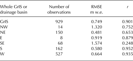
The PROMICE observations (Machguth and others, Reference Machguth2016) have again been used to assess the VS-1 model results on the full 1 km ice mask and for the glaciers in each drainage basin. These are shown in Figure 9 with RMSE and r in Table 6. Figure 9 shows broadly as strong a correlation between VS-1 and observed as we obtained for just those observations on the common ice mask, Figure 7a. Table 6 shows that the error for all observations on the 1 km ice mask is slightly worse, 0.749 m w.e., than it was for just the common mask, 0.736 m w.e., and the correlation is higher, 0.901 m w.e., on the full 1 km mask compared with 0.754 m w.e. on the common mask. We can therefore be confident that VS-1 is modelling SMB well over as much of the GrIS as we can assess. Looking at a more regional level there are naturally differences. Some drainage basins have few observations and so are difficult to draw conclusions from, but for all basins with more than 100 observations RMSE is 0.664 m w.e. or lower, i.e. better than that for the whole GrIS. It is the northwest, east and southeast basins that have poorer RMSE. As discussed previously in Section 3.1.2, glaciers 254 (Hellheim) in the southeast and 475 (Tuto Ramp) in the northwest are outliers almost certainly due to the precipitation used in VS-1. Glacier 232 (Violin Glacier) in the east is likely to be similarly affected. Therefore in those drainage basins where there is a large amount of data from multiple glaciers errors are low for VS-1, adding to our confidence in this method.
Table 6. RMSE and Pearson's correlation coefficient of VS-1 model vs measured SMB for PROMICE observations at sites on the full 1 km ice mask, for all data and by drainage basin as shown in Figure 8
3.3. Glacier scale runoff
Using the 1 km resolution PDD method, we now focus on specific glaciers or groups of glaciers. We take two examples: Jakobshavn Isbræ on the west coast and the region around Helheim Glacier on the east coast of Greenland. Possible relationships between runoff and iceberg calving for the GrIS as a whole with multi-year averaged data have previously been proposed (Bamber and others, Reference Bamber, van den Broeke, Ettema, Lenaerts and Rignot2012; Box and Colgan, Reference Box and Colgan2013). Increased runoff may potentially increase calving rates via a number of mechanisms (Box and Colgan, Reference Box and Colgan2013). Meltwater penetration to the glacier bed may increase lubrication and glacier speed, contribute to the undercutting of calving fronts when meltwater enters the ocean, decrease glacier structural integrity through increased crevasse extent and over many years may soften the ice by warming it. Conversely there may also be a negative effect of runoff on calving since ice that melts as runoff is removed from the glacier before it reaches the calving front (Goelzer and others, Reference Goelzer2013), and there may also be a decrease in iceflow after an initial meltwater increase once subglacial drainage becomes more efficient (Sundal and others, Reference Sundal2011). Therefore we use our high spatial resolution results to investigate possible correlations between runoff and calving in these two areas.
The locations of the two regions considered here are indicated in Figure 1 and in Figure 10 we show the specific areas, with elevation contours, over which runoff has been calculated for correlation with calving. The Jakobshavn Isbræ area is defined as between 68.8–69.5°N and 48.3–50.5°W. The Helheim glacier area is defined as between 66.2–67.0°N and 36.4–39.0°W. In Figure 11a we compare local annual runoff for Jakobshavn Isbræ with the variation in the up-glacier position of the summer (May–September) calving front from Csatho and others (Reference Csatho, Schenk, van der Veen and Krabill2008) (when multiple measurements were quoted for a single year, we take the mean). While iceberg calving is not the only process responsible for change in the calving front position, with glacier speed and thickness also contributing, a steady calving front position might intuitively be expected to be consistent with stable rates of annual iceberg discharge, while rapid retreat/advance should correspond to an increase/decrease in calving, respectively. The calving front data date back to 1946 but there are many years without data. In Figure 11b we compare local annual runoff for Helheim Glacier with a calving flux proxy derived from sedimentary deposits in Sermilik Fjord (Andresen and others, Reference Andresen2012). We take an area that includes Helheim, Fenris and Midgard glaciers, although Helheim Glacier is the major source of icebergs in the fjord (Andresen and others, Reference Andresen2012). The calving flux data are from 1890 with some missing years. For both glaciers there appear to be correlations between runoff and calving, as shown in Figure 11. For Jakobshavn Isbræ, Figure 12a, r = 0.48, and for Helheim Glacier, Figure 12b, r = 0.33. If these data are detrended the correlations are reduced to r = 0.43 for Jakobshavn Isbræ and r = 0.15 for Helheim Glacier. The former is statistically significant at the 95% confidence level but the latter only at 86%. Higher de-trended correlations may be found if, rather than considering runoff over the entire areas, we restrict attention to lower elevations, as shown in Table 7. Intuitively one might expect better correlation between calving and runoff for lower elevation range runoff since the ice at the lowest elevations is that closest to the calving front. However we only see this for Helheim Glacier where the correlation becomes statistically significant with 95%, or higher, confidence level when runoff is restricted to below 750 m. For Jakobshavn Isbræ the correlation gets less significant with a lower range of elevation runoff. The reasons why the statistical correlations for the two glaciers differ in this respect are not obvious and while this may be of interest for further work the important result here is that for both glaciers a positive correlation between local runoff and calving flux can be found, albeit in one case only if we restrict runoff to lower elevations. However it is clear from Figure 10 that in both cases runoff and calving data show significant increase from the mid-1990s onwards and are less well correlated beforehand. For Jakobshavn Isbræ there are many years with no calving front data prior to 1985: therefore we cannot be sure how well discharge is correlated with runoff, and we can also see a retreat (positive change) in calving front position of 2.3 km from 1988 to 1992 at the same time as annual runoff decreases by 315 Gt a−1, and again from 1992 to 1997 the calving front advances (negative change) by 3.8 km while runoff increases by 421 Gt a−1. Similarly for Helheim Glacier we can see periods of sharp increases in calving flux without corresponding increases in runoff around 1939 and 1978 and it is only from 1996 onwards that both quantities increase consistently. Therefore any overall high correlation between runoff and calving flux or front retreat could be unduly influenced by corresponding high values in both variables after the mid to late 1990s and high correlation between two variables does not necessarily imply a causal link. Our results could be an indication of a possible nonlinear link between runoff or SMB and GrIS iceberg discharge, the nature of which may have changed over time, as found by Bigg and others (Reference Bigg2014) and Zhao and others (Reference Zhao2016), whereby SMB, or in our case runoff, has been a factor influencing GrIS calving throughout the 20th century but with varying importance, becoming more significant in recent years.
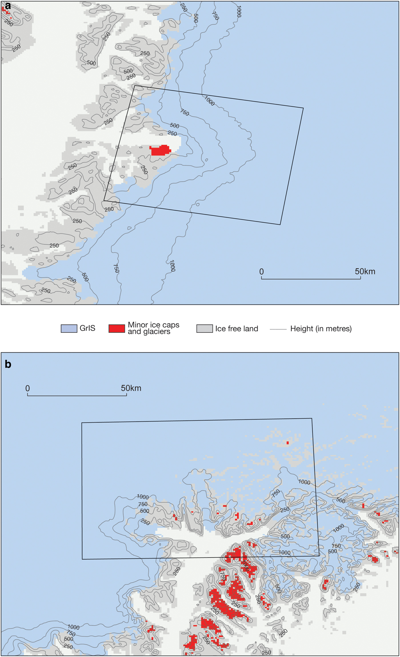
Fig. 10. The 1 km ice mask zoomed in onto the area around (a) Jakobshavn Isbræ and (b) Helheim Glacier with contour lines showing elevation in m and the areas used to calculate average runoff in Section 3.3 indicated within the boxes.
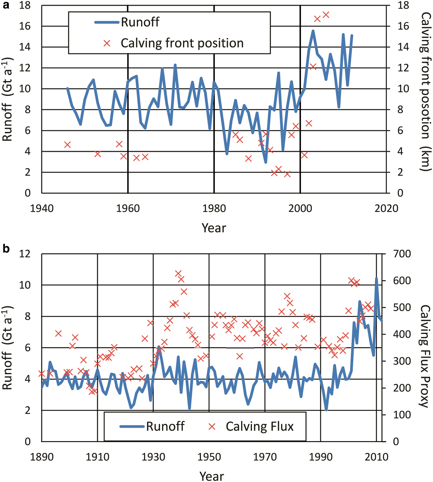
Fig. 11. Correlation between annual runoff and calving data for the areas around specific glaciers, as defined in main text. a) Jakobshavn Isbræ, compared to calving front position measured up glacier, (Csatho and others, 2008), and b) Helheim Glacier compared to calving flux proxy, sand deposition rate (g m−2 a−1) (Andresen and others, 2012).
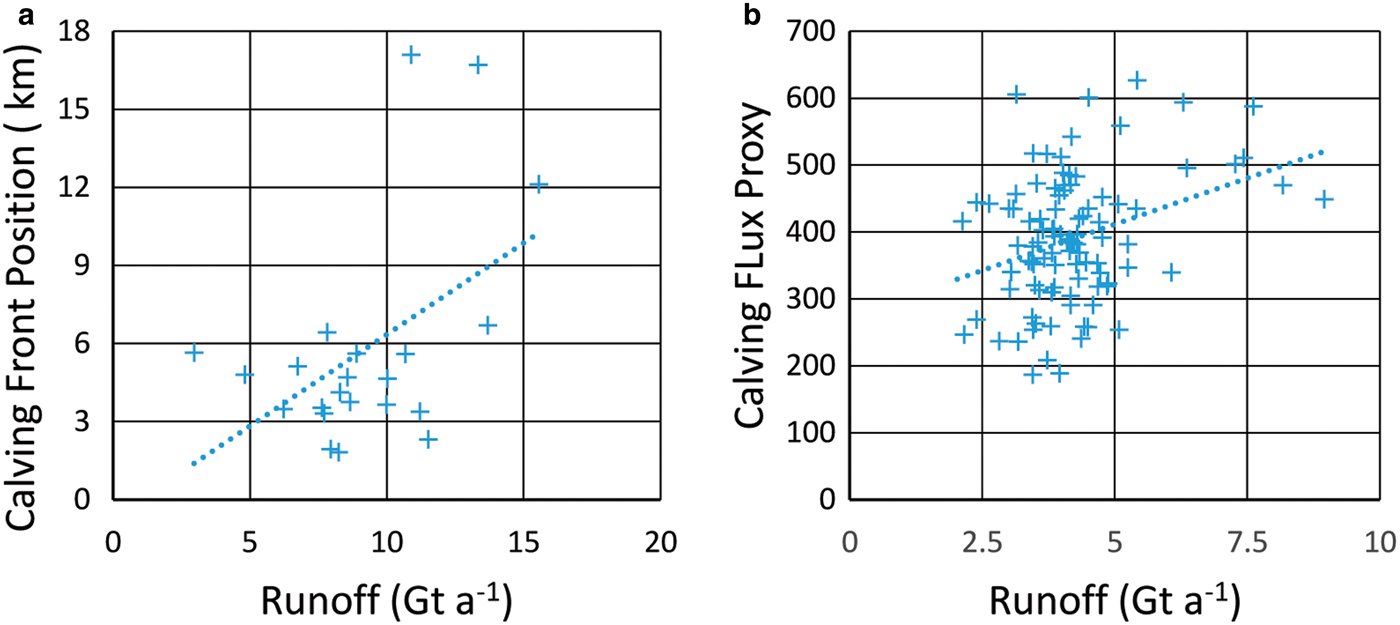
Fig. 12. Scatter plots, with linear trend lines, showing the correlation between annual runoff and calving data for the areas around specific glaciers, as defined in main text. (a) Jakobshavn Isbræ, compared with calving front position (Csatho and others, Reference Csatho, Schenk, van der Veen and Krabill2008) and (b) Helheim Glacier, compared with calving flux proxy, sand deposition rate (g m−2 a−1) (Andresen and others, Reference Andresen2012).
Table 7. Correlation and statistical significance between runoff and calving
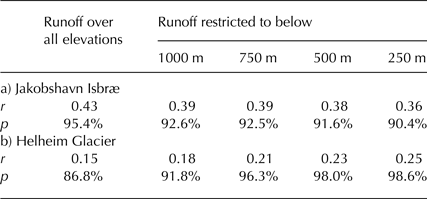
Pearson's correlation coefficient, r, and level of statistical confidence, p, between annual runoff and calving data for the areas around specific glaciers, as defined in main text. (a) Jakobshavn Isbræ, compared with calving front position, (Csatho and others, Reference Csatho, Schenk, van der Veen and Krabill2008), and (b) Helheim Glacier, compared with calving flux proxy, (Andresen and others, Reference Andresen2012). Runoff is measured over the entire area defined and restricted to a maximum elevation as shown. Data are detrended and are for the range of years covered by the appropriate calving data. That is for (a) 1946–2006 and (b) 1890–2008.
4. SUMMARY AND CONCLUSIONS
We have shown that using a PDD model to calculate SMB of the GrIS at a high spatial resolution of 1 km × 1 km compared with a previous work at 5 km × 5 km spatial resolution leads to higher runoff and therefore lower SMB due to lower-elevation areas on the edge of the ice sheet being better resolved. Conversely, employing a more realistic parameterization of daily temperature variation than one that assumes a constant standard deviation leads to lower runoff and therefore higher SMB, in line with previous work (Rogozhina and Rau, Reference Rogozhina and Rau2014; Jowett and others, Reference Jowett, Hanna, Ng, Huybrechts and Janssens2015). In comparison with RCMs on an identical ice mask our PDD model shows similar SMB values for most years, and all three models show statistically similar SMB declines for the whole period since 1979 and the subperiod of strong Greenland warming from 1998. The main components of SMB, precipitation and runoff, are both lower for our model than the corresponding values from RCMs, and so we call for further concerted efforts to collect key in situ validation data from across the ice sheet to resolve these model differences, as some key regions (e.g. interior southeast Greenland) are still largely lacking such data. The results of the comparison of modelled SMB with in situ (PROMICE) observations suggest that the RCMs may be more accurate at local level, in some areas, than the PDD model approach. However, the generally robust PROMICE comparison with the VS-1 model gives confidence in the long timescales presented here for the VS-1 model, for which RCMs are impractical at such a high, 1 km × 1 km, spatial resolution. When we examine the GrIS SMB at the drainage basin scale over 1870–2012 we see that all parts of the ice sheet are experiencing increased runoff and therefore decreased SMB over the last decade, with some years and drainage basins even showing a negative SMB. Basins in the north show a clear drop in SMB ~1930. The south and eastern basins have a more constant SMB but peak around the 1940s with the former basin having a sharper decrease post 1970. The west basin's SMB peaks in the 1920s and thereafter decreases with that decrease accelerating after 2000. We have also examined runoff at the glacier scale. For the Jakobshavn Isbræ and Helheim glaciers we show that correlations can be found between runoff and either calving front retreat or calving flux, respectively, for these two glaciers, but this trend is most noticeable from the mid-1990s.
Further work will go beyond using downscaled meteorological reanalyses to combine our optimized statistical downscaling/SMB modelling with an RCM-based approach. An advantage of the SMB modelling approach presented here is that it enables us to examine GrIS SMB changes on the relatively long, multi-decadal timescale at a reasonable (monthly) temporal resolution across a wide range of spatial scales, compared with what is presently possible for purely RCM-based studies at spatial resolutions of ~10 km × 10 km. For example the PDD approach could be more easily used in conjunction with multiple future climate scenarios. Therefore our SMB model output should help shed light on the evolution and sensitivity of GrIS SMB in response to multiple climatic forcing factors over the past few years to more than a century. Also, in accordance with earlier work (e.g. Vernon and others, Reference Vernon2013), our results clearly show that more detailed and rigorous SMB intercomparison studies are essential to help narrow the uncertainty in absolute SMB values and Greenland's overall recent ice mass change.
ACKNOWLEDGEMENTS
Funding was provided by the Natural Environment Research Council (NERC) grant NE/H023402/1. 20th Century Reanalysis V2 data were provided by the NOAA/OAR/ESRL PSD, Boulder, Colorado, USA, from their Web site at http://www.esrl.noaa.gov/psd/. Support for the 20th Century Reanalysis Project dataset is provided by the U.S. Department of Energy, Office of Science Innovative and Novel Computational Impact on Theory and Experiment (DOE INCITE) program, and Office of Biological and Environmental Research (BER), and by the National Oceanic and Atmospheric Administration Climate Program Office. We thank the British Atmospheric Data Centre, and through them, ECMWF, for allowing us to access the ECMWF reanalyses. Data from the Programme for Monitoring of the Greenland ice sheet (PROMICE) were provided by the Geological Survey of Denmark and Greenland at http://www.promice.dk. We also thank Jonathan Bamber for providing the 1 km resolution ice mask and DEM used, Valentina Barletta for the drainage basin mask and Camilla Andresen for providing us with the Helheim calving flux data. We also thank the anonymous referees for their advice in improving this manuscript.


 Open access