


1. Introduction
Fluid–structure interactions lead to many important phenomena in engineering applications, including the vortex-induced vibrations (VIVs) and vortex-induced rotations (VIRs). Both VIVs and VIRs are simplified but fundamental models for understanding the mechanisms of fluid–structure interactions. In this section we will briefly revisit the literature to explain the related concepts, and to clarify the motivation of the present study.
There have been extensive experimental and numerical investigations on VIVs in past years (Sarpkaya Reference Sarpkaya2004; Williamson & Govardhan Reference Williamson and Govardhan2004). In these studies, circular cylinder is the simplest model but can already lead to typical VIV phenomena. Griffin (Reference Griffin1985) and Williamson & Roshko (Reference Williamson and Roshko1988) investigated systematically the fluctuating lift and drag forces on a two-dimensional cylinder in a uniform cross-flow, coupled with the alternate vortex shedding with three typical patterns, i.e. the 2S mode, 2P mode and P+S mode, respectively. These results were validated by using numerical simulations (Minewitsch, Franke & Rodi Reference Minewitsch, Franke and Rodi1994; Taylor & Vezza Reference Taylor and Vezza1999). As one of the most interesting phenomena of VIVs, the frequency lock-in has been systematically studied. As an example, considering the transverse oscillation of a circular cylinder, discussions on the parameter influences can be found in Bearman (Reference Bearman2011). Towards complicated reality, there have also been many studies on the VIVs of square cylinders (Cheng, Zhou & Zhang Reference Cheng, Zhou and Zhang2003; Amandolèse & Hémon Reference Amandolèse and Hémon2010; Bao, Wu & Zhou Reference Bao, Wu and Zhou2012; Jiang et al. Reference Jiang, Andreopoulos, Lee and Wang2016; Zhang et al. Reference Zhang, Mao, Song, Ding and Tian2018; Han & de Langre Reference Han and de Langre2022; Qiu et al. Reference Qiu, Xu, Du, Zhao and Lin2022) and multiple objects (Mittal, Kumar & Raghuvanshi Reference Mittal, Kumar and Raghuvanshi1997; Assi, Bearman & Meneghini Reference Assi, Bearman and Meneghini2010). By comparing with a single circular cylinder, these results reveal more complicated VIVs, where the responses of objects are affected by additional setting parameters.
On the other hand, the investigations on VIRs are not so broad by comparison with VIVs. There exist some investigations on the VIRs of typical shapes of freely rotating cylinders, such as circular cylinders (Juarez et al. Reference Juarez, Scott, Metcalfe and Bagheri2000), triangular cylinders (Wang et al. Reference Wang, Zhu, Zhang and He2011, Reference Wang, Yan, Chen, Ji and Zhai2019) and rectangular cylinders (Robertson et al. Reference Robertson, Li, Sherwin and Bearman2003). However, the most common model for studying VIRs is to use square cylinders. Early experimental and numerical studies by Zaki, Sen & Gad-El-Hak (Reference Zaki, Sen and Gad-El-Hak1994) recognized four typical modes of square cylinder response, i.e. static stability, oscillation, reverse rotation and autorotation, respectively. A systematic study was performed by Ryu & Iaccarino (Reference Ryu and Iaccarino2017) and enriched the response modes into six characteristic regimes through a parameter investigation, i.e. stable, small-amplitude oscillation,  ${\rm \pi} /2$-limit oscillation, random rotation, ${\rm \pi}$-limit oscillation and autorotation regimes, respectively. Comparing with Zaki et al. (Reference Zaki, Sen and Gad-El-Hak1994), this classification showed more details and complexities at moderate Reynolds numbers, by discussing the phase synchronization/differences between the moment generation and angle of rotation in different regimes. There also exist other studies considering more complicated cases, such as the combination of square cylinders (Shao et al. Reference Shao, Shu, Liu and Zhao2019) and rotation in a microchannel (Pan, Chen & Wu Reference Pan, Chen and Wu2019). Similar to the VIVs, these complicated settings lead to different response of the square cylinder, but the responses were not beyond the classification of Ryu & Iaccarino (Reference Ryu and Iaccarino2017). In the present paper we will show more complicated response of a single cylinder by expanding the parameter space. In fact, Ryu & Iaccarino (Reference Ryu and Iaccarino2017) remarked that the rotational inertia of a square cylinder, which can also be dimensionlessly parameterized to the density ratio between cylinder and fluid, might also affect the dynamics responses of a square cylinder, but almost all existing studies used a constant rotational inertia. Expanding the parameter space by considering the change of rotational inertia will then be performed in the present paper, aiming at revealing new response modes and underlying mechanisms in VIRs.
Some phenomena of VIRs are analogous to VIVs, for example, the small-amplitude oscillation regime of square cylinders can also be considered as an angular vibration and analytically predicted by introducing a free-streamline boundary-layer model (Luo et al. Reference Luo, Mou, Huang, Huang and Fang2023), where the elastic force is not generated by a solid property, but is the result of a flow field. In this sense, the autorotation regime shows its particularity by comparing with the phenomena in VIVs and has attracted many investigations, for example Lugt (Reference Lugt1980, Reference Lugt1983), Ryu (Reference Ryu2018) and Xia et al. (Reference Xia, Lin, Ku and Chan2018). In the present paper, we will also contribute to this understanding. Specifically, we will show a ‘wavy rotation’ regime, which is similar to the autorotation regime but contains periodically short-time back swing.
This paper is organized as follows: the problem formation and computational method are described in § 2; the results and discussion are presented in § 3; finally, in § 4 we give the conclusions.
2. Problem description and numerical method
In the present paper, we consider a two-dimensional case that a uniform incompressible flow passes and interacts with a freely rotatable rigid square cylinder, as sketched in figure 1. The streamwise and normal directions are denoted as  $x$ and $y$, respectively. The square cylinder, with side length $L$, can freely rotate around its centre $O$, which is located $8.5L$ from the inlet in the streamwise direction, and in the centre in the normal direction. The computational domain size is $32L\times 16L$, with all boundaries having the free stream velocity condition, i.e. $\boldsymbol {u}=(u_\infty,0)$ with $\boldsymbol {u}$ being the flow velocity. The flow field is governed by the incompressible Navier–Stokes equations,
 $$\begin{gather} \boldsymbol{\nabla}\boldsymbol{\cdot}\boldsymbol{u}=0, \end{gather}$$
 $$\begin{gather}\rho_0\left(\frac{\partial \boldsymbol{u}}{\partial t}+\boldsymbol{u}\boldsymbol{\cdot}\boldsymbol{\nabla}\boldsymbol{u}\right)={-} \boldsymbol{\nabla} p+\mu\Delta\boldsymbol{u}+\boldsymbol{f}, \end{gather}$$
with flow parameters  $\rho _0$ the fluid density and $\mu$ the dynamics viscosity. Here $t$ is the time, $p$ is the pressure and $\boldsymbol {f}$ is the momentum forcing applied to enforce the no-slip boundary condition along the immersed boundary.

Figure 1. Schematic diagram of rigid square cylinder moving in a uniform flow with velocity  $u_{\infty }$.
According to the theorem of angular momentum, the governing equation for a freely rotatable rigid body is
 \begin{equation} I\frac{\mathrm{d}^2\theta}{\mathrm{d}\kern 0.06em t^{2}}=T, \end{equation}
where  $I$ is the moment of inertia about the centre of the cylinder, $\theta$ is the rotation angle and $T = |\boldsymbol {T}|$ is the torque exerted on the mass by the fluid. For the case of a square cylinder we can write
 $$\begin{gather} I=\rho_s{L^{4}}/6, \end{gather}$$
 $$\begin{gather}\boldsymbol{T}=\int_{\varGamma}\boldsymbol{F}\times\boldsymbol{X}_{r}\,\mathrm{d}\kern 0.06em s, \end{gather}$$
where  $\rho _s$ is the density of the cylinder, $\varGamma$ is the boundary of the cylinder, $\boldsymbol {F}$ is the Lagrangian force exerted on the cylinder surface and $\boldsymbol {X}_{r}$ is the displacement vector with the centre of the cylinder. Substituting (2.4) into (2.3) leads to
 \begin{equation} T=\frac{1}{6}\rho_s{L^4}\frac{\mathrm{d}^2\theta}{\mathrm{d}t^{2}}. \end{equation}
The non-dimensionalization on the above equations is performed by introducing the following characteristic scales:  $u_{\infty }$ for velocity; $L$ for length; $\rho _0$ for fluid density; $L/u_{\infty }$ for $t$;
$t$;  ${\rho _0}u^2_{\infty }$ for $p$;
$p$;  ${\rho _0}u^2_{\infty }/L$ for $\boldsymbol {f}$; ${\rho _0}{u^2_{\infty }}$ for $\boldsymbol {F}$; ${\rho _0}{L^4}$ for $I$;
$I$;  ${\rho _0}{u^2_{\infty }}L^2$ for $\boldsymbol {T}$. The non-dimensional governing equations are therefore
 $$\begin{gather} \frac{\partial\boldsymbol{u}^*}{\partial t^* }+\boldsymbol{u}^*\boldsymbol{\cdot}\boldsymbol{\nabla}^*\boldsymbol{u}^*={-}\boldsymbol{\nabla^*}{p^*}+ \frac{1}{Re}\varDelta^*{\boldsymbol{u}^*}+\boldsymbol{f^*}, \end{gather}$$
 $$\begin{gather}\frac{1}{6}\rho\frac{\mathrm{d}^2\theta}{\mathrm{d}t^{*2}}=T^*, \end{gather}$$
where  ${Re}={\rho _0 u_{\infty }L}/{\mu }$ is the Reynolds number, and $\rho =\rho _s/\rho _0$ is the non-dimensional solid density. The initial condition of the cylinder is set as $\theta |_{t=0}=\theta _0$ and ${\rm d}\theta /{\rm d}t|_{t=0}=0$.
The interaction between the fluid and the immersed boundary is described by introducing the Lagrangian force, calculated as
 \begin{equation} \boldsymbol{F}^*=\alpha \int_{0}^{t^*} (\boldsymbol{U}_{ib}^*-\boldsymbol{U}_s^*)\,\mathrm{d}t'-\beta (\boldsymbol{U}_{ib}^*-\boldsymbol{U}_s^*), \end{equation}
where  $\alpha$ and $\beta$ are negative constants, $\boldsymbol {U}_s^*$ is the velocity of the cylinder boundary and $\boldsymbol {U}_{ib}^*$ is the fluid velocity obtained by interpolation at the immersed boundary, which is expressed as
 \begin{equation} \boldsymbol{U}_{ib}^* (s,t)= \int_{\varOmega} \boldsymbol{u}^* (\boldsymbol{x},t)\delta{ (\boldsymbol{X}(s,t)-\boldsymbol{x})}\,\mathrm{d}\kern 0.06em \boldsymbol{x} \end{equation}
with  $\delta ()$ the Dirac delta function (in calculations we use a smoothed delta function instead). The relation between Lagrangian force and Eulerian force is
 \begin{equation} \boldsymbol{f}^* (\boldsymbol{x},t)=\int_{\varGamma} \boldsymbol{F}^* (s,t)\delta (\boldsymbol{x}-\boldsymbol{X} (s,t))\,\mathrm{d}\kern 0.06em s. \end{equation}
The details on the immersed boundary method and numerical discretizations can be found in Huang, Shin & Sung (Reference Huang, Shin and Sung2007).
In order to verify the correctness of the calculation, we calculate the case where flow passes a fixed square cylinder. The Reynolds number is  ${Re}=100$. Mesh and calculation domain independence is verified in table 1. It is shown that when the calculation domain is larger than $16L\times 32L$, and the grid number is more than $512\times 1024$, the aerodynamic performances, including the mean drag coefficient $C_D$, root-mean-square (r.m.s.) lift coefficient $C_{L,rms}$ and Strouhal number ${St}$, can converge.
Table 1. Comparison of mean drag coefficient  $C_D$, r.m.s. lift coefficient $C_{L,{rms}}$ and Strouhal number ${St}$ under different computational domains and grid numbers. Reynolds number ${Re}=100$.

To assess the accuracy of the code, we select the case with  $512\times 1024$ grids, in a ${16L\times 32L}$ calculation domain, and simulate a fixed, rigid square cylinder in a two-dimensional uniform cross-flow. Compared with the results in the literature, as shown in table 2, a good agreement can be observed to support the present calculations.
Table 2. Comparison of mean drag coefficient  $C_D$, r.m.s. lift coefficient $C_{L,{rms}}$ and Strouhal number ${St}$ with reference results, for the case that flow passes a fixed square cylinder. Reynolds number ${Re}=100$. The present calculation is performed with $512\times 1024$ grids, in a $16L\times 32L$ calculation domain.

Further validations by comparing with Ryu & Iaccarino (Reference Ryu and Iaccarino2017) are performed at different Reynolds numbers, respectively, as shown in figure 2. In the insets we plot the relative differences between them, which are always less than 4 %. This value is small by comparison with the literature (see table 2), indicating the correctness of the present results.

Figure 2. Comparison of (a) drag coefficient (b) lift coefficient with Ryu & Iaccarino (Reference Ryu and Iaccarino2017) at Reynolds number from 45 to 150, respectively. The insets show the relative difference between the present study and the reference work.
In the following parts, we perform calculations on the freely rotatable square cylinder under various parameters of  $0.1\leqslant \rho \leqslant 10$ and $40\leqslant Re\leqslant 150$.
3. Results
In order to better describe and analyse the phenomena, here we first define two terms. Following Park et al. (Reference Park, Min, Ha and Yoon2015), Ryu & Iaccarino (Reference Ryu and Iaccarino2017), Pan et al. (Reference Pan, Chen and Wu2019) and Shao et al. (Reference Shao, Shu, Liu and Zhao2019), we use ‘regime’ to refer to the dynamic responses of the square cylinder; by contrast, the term ‘region’ is used to describe an area in the  $(\rho, {Re})$ phase plane, for the ease of following discussions. As will be shown in the following parts, ‘region’ and ‘regime’ are not a bijection. We will discuss the regimes in § 3.1 and show the regime map by defining the regions in § 3.2.
3.1. Regimes of dynamic responses of a square cylinder
In this subsection we will summarize and classify the regimes we observed in calculations. We follow Ryu & Iaccarino (Reference Ryu and Iaccarino2017) to define six regimes, i.e. stable, small-amplitude oscillation,  ${\rm \pi} /2$-limit oscillation, random rotation, ${\rm \pi}$-limit oscillation and autorotation regimes. Note that these definitions are not exactly the same as Ryu & Iaccarino (Reference Ryu and Iaccarino2017), for example, we observe different dynamic responses in the ${\rm \pi}$-limit oscillation regime. Besides, we will show two new regimes, i.e. wavy rotation and transition regimes, which, to our knowledge, have not been reported in the literature.
These typical regimes are presented in figure 3, by selecting some typical combinations  $(\rho, {Re})$. Their descriptions are listed as follows.
(a) The stable regime indicates that the initial perturbation is damped, and the square cylinder reaches a stable equilibrium point.
(b) The small-amplitude oscillation regime indicates that the square cylinder oscillates monoharmonically with small amplitudes less than $10^{-2}$. This threshold value is consistent with Ryu & Iaccarino (Reference Ryu and Iaccarino2017).
(c) The
${\rm \pi} /2$-limit oscillation regime indicates that the amplitude of the rotation angle is close to $\pm {\rm \pi}/4$. In addition, multiharmonic oscillations can be observed.(d) The transition regime can be considered as a mixture of the
${\rm \pi} /2$-limit oscillation and random rotation regimes. Specifically, the regime randomly switches between different quasi-${\rm \pi} /2$-limit oscillation regimes with different quasiequilibrium angles.(e) The random rotation regime indicates intermittent oscillations and rotations in a temporally random fashion. Comparing with the transition regime, no quasi-
${\rm \pi} /2$-limit oscillation can be observed.(f) The
${\rm \pi}$-limit oscillation regime indicates another temporal oscillation of the cylinder with a rotation limit ${\rm \pi}$. The cylinder may oscillate or rotate in a random fashion at the beginning, and then oscillates periodically. Note that Ryu & Iaccarino (Reference Ryu and Iaccarino2017) reported that the ${\rm \pi}$-limit oscillation regime always contains a single bell-like curve in each period, but we also find other subregimes with multiple peaks and valleys in a period (see the dashed line in figure 3f as an example). The details of these phenomena will be analysed in § 3.4.3.(g) The wavy rotation regime indicates that in a period, the cylinder rotates for a large angle in a certain direction and then reverses for a small angle. According to symmetry, the rotation direction of the cylinder can be clockwise or anticlockwise. In addition, we also find another subregimes of this regime which reverses two times in one period (see discussions later in § 3.4.2).
(h) The autorotation regime indicates that the cylinder undergoes random rotations at the beginning and then autorotates in one direction without reversal. According to symmetry, the rotation direction of the cylinder can be clockwise or anticlockwise.


Figure 3. Time histories of rotation angle of typical regimes: (a) stable regime ( ${Re}=40,\rho =2$); (b) small-amplitude oscillation regime ( ${Re}=70,\rho =10$); (c) ${\rm \pi} /2$-limit oscillation regime ( ${Re}=80,\rho =2$); (d) transition regime (solid line, ${Re}=90,\rho =4$; dashed line, ${Re}=100,\rho =1$); (e) random rotation regime ( ${Re}=100,\rho =2$); (f) ${\rm \pi}$-limit oscillation regime (solid line (1-peak subregime), ${Re}=130,\rho =1$; dashed line (2-peak subregime), ${Re}=140,\rho =3.1$); (g) wavy rotation regime (solid line, ${Re}=140,\rho =2.5$; dashed line, ${Re}=140,\rho =2.6$); (h) autorotation regime (solid line, ${Re}=150,\rho =2$; dashed line, ${Re}=150,\rho =0.1$).
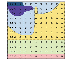
3.2. Overview of the region map of regimes
Based on our calculations, we summarize the regimes under different Reynolds numbers and density ratios in figure 4. Each symbol corresponds to a numerical test case, while the different symbol styles are used to represent different regimes. Based on these results, we further divide the  $(\rho, {Re})$ phase plane into six regions (contours in figure 4). Their descriptions are listed as follows.

Figure 4. Overview of regimes on the  $(\rho, {Re})$ phase plane. According to the regimes, the phase plane is further divided into six regions. The cases with $\rho =2$ correspond to the set-up of Ryu & Iaccarino (Reference Ryu and Iaccarino2017).
Region (1) corresponds to the stable regime at  ${Re}=40$. Changing the value of $\rho$ does not affect the regime.
Region (2) corresponds to the small-amplitude oscillation regime. Again, changing the value of  $\rho$ does not affect the regime.
Region (3) corresponds to the  ${\rm \pi} /2$-limit oscillation regime. According to figure 4, it is interesting that an irregular tooth-like shape is observed at $\rho =5$ and ${Re}=130, 140$. This phenomenon will be explained later in § 3.3.
Region (4) corresponds to both the transition and random rotation regimes. We classify these two regimes in the same region since both of them correspond to unstable motions of the cylinder.
Region (5) is complicated since there exists four regimes chaotically, i.e. random rotation,  ${\rm \pi}$-limit oscillation, wavy rotation and autorotation regimes. In figure 4 we present seven test cases as ‘multiple regimes’, but indeed we have calculated many more cases in this region and found that the results are quite uncertain. For instance, in figure 5 we show the regimes of 40 test cases for ${Re}=140$ and $\rho \leqslant 4$. It can be observed that regimes are chaotic. In addition, we can observe different dynamics for the ${\rm \pi}$-limit oscillation and wavy rotation regimes in this region, in which one period can contain multiple peaks. These different dynamics have not been discussed in the literature, and they will be named as ‘subregimes’ in the present study. The complexity in this region is also reflected from the fact that different initial angles of the cylinder can lead to different regimes (see discussions in § 3.5).

Figure 5. Regimes and subregimes for the cases of  ${Re}=140, \rho \leqslant 4$. Initial angle is selected as $\theta _0=0.1$.
Region (6) corresponds to the autorotation regime.
We remark that Ryu & Iaccarino (Reference Ryu and Iaccarino2017) have defined a classification for the  $\rho =2$ cases. Here our classifications are principally consistent with Ryu & Iaccarino (Reference Ryu and Iaccarino2017), while the differences are mainly due to the slight differences in the definition of regimes.
In the following subsections, we will first discuss the tooth-like shape of the  ${\rm \pi} /2$-limit oscillation regime, and then visit in detail the typical regions in figure 4.
3.3. Tooth-like shape in the regime map
As summarized in § 3.2, an interesting phenomenon in the region map of regimes is the irregular tooth-like shape of region (3), which is located at  $\rho =5$ and ${Re}=130, 140$. In order to understand why these parameters lead to the ${\rm \pi} /2$-limit oscillation regime instead of the transition or random rotation regimes, an analysis of the frequency spectrum on the dynamic responses of the square cylinder is carried out.
At Reynolds number  ${Re}=120$, we select two typical cases with $\rho =5$ and $6$. It can be found from figure 4 that both cases lead to ${\rm \pi} /2$-limit oscillation, hence it is possible to transfer the time evolution of the lift coefficient (shown in figures 6a and 6b, respectively) to frequency space. As seen from figures 6(c) and 6(d), both cases have two main frequencies. This is qualitatively consistent with the observations of Ryu & Iaccarino (Reference Ryu and Iaccarino2017) for lower Reynolds number ${Re}=90$, but here the two main frequencies have comparable amplitudes, rather than the quasimonofrequency responses in Ryu & Iaccarino (Reference Ryu and Iaccarino2017). In fact, in Ryu & Iaccarino (Reference Ryu and Iaccarino2017) the main frequency was shown to correspond to the vortex shedding frequency, while the small-amplitude small-frequency envelope was weak, and was not explained. By contrast, in our cases both frequencies have their amplitudes at the same order, leading to the transition to other complicated regimes.

Figure 6. Comparison between (a)  ${Re}=120,\rho =5$ and (b) ${Re}=120, \rho =6$, showing (i) the evolution of lift coefficient $C_L$ and (ii) its frequency spectrum.
Clearly, by naming the frequency of largest amplitude as ‘basic frequency’, and the other one as ‘subfrequency’, the comparison between figures 6(c) and 6(d) shows their different orders. We can perform the same operation on all cases with  ${\rm \pi} /2$-limit oscillation regime near the tooth-like shape in the regime map, as shown in table 3. It is interesting that for all the $\rho =5$ cases the basic frequency is always smaller than the subfrequency, while for other cases it is the opposite. In table 3 we also use the reference frequencies of the lift coefficient evolution in the flow past a fixed circular cylinder (denoted as RF1) and square cylinders (denoted as RF2 and RF3) as references, which could approximately represent the frequencies of natural vortex shedding. It can be found that for the $\rho =5$ cases the subfrequency is close to the reference frequencies, while for other cases the basic frequency is close to the reference frequencies. We can therefore explain that the transition from ${\rm \pi} /2$-limit oscillation regime to other unstable regimes can be related to the interaction between the cylinder and the natural vortex shedding. For the $\rho \ne 5$ cases, the basic frequency is close to the reference frequencies, indicating that the influence of natural vortex shedding is dominant. Hence, increasing the Reynolds number will lead to instability of natural vortex shedding and then a change of the regime of the cylinder. By contrast, for the $\rho =5$ cases the dominant factor for the cylinder response is a lower-frequency envelope, therefore the instability of natural vortex shedding will be more difficult to change the regime of the cylinder.
Table 3. Comparison of main frequencies of lift coefficient evolution in different cases. Here, RF1 refers to the reference frequency of lift coefficient evolution in the flow past a fixed circular cylinder (Williamson Reference Williamson1989); RF2 and RF3 refer to the reference frequency of lift coefficient evolution in the flow past a fixed square cylinder with angle  $0$ and ${\rm \pi} /4$, respectively. The sign * corresponds to transition or random rotation regimes without any main frequency.

In brief, the comparison of the frequency with that of vortex shedding can explain the formation of the tooth-like shape of the  ${\rm \pi} /2$-limit oscillation regime.
3.4. Moment-generating mechanisms of new regimes and subregimes
As summarized in § 3.1, in the present study we have observed new regimes and subregimes for the cylinder responses. In this section we will follow the analysis method of Ryu & Iaccarino (Reference Ryu and Iaccarino2017), to show the underlying moment-generating mechanisms of these regimes and subregimes.
3.4.1. Transition regime
As shown in figure 3(d), the typical dynamics of the transition regime indicates that the regime randomly switches between different quasi- ${\rm \pi} /2$-limit oscillation regimes with different quasiequilibrium angles. Since the dynamics of the ${\rm \pi} /2$-limit oscillation regime has already be analysed with substantial details in Ryu & Iaccarino (Reference Ryu and Iaccarino2017), here we will emphasize the switch procedure and the corresponding moment-generating mechanisms, as presented in figure 7. In the figure we show the time history of the rotation angle ( $\theta$), the non-dimensional angular velocity ${\omega }$ (defined as ${\omega }^*L/u_{\infty }$) and the moment coefficient $C_m$ (defined as $2{T^*}/{\rho _0}{u^2_{\infty }}L^2$). Seven typical instants (A–G) are marked. Between $A$ and $C$, the square cylinder is driven by the out-of-phase synchronized moments, as the same as the ${\rm \pi} /2$-limit oscillation regime described by Ryu & Iaccarino (Reference Ryu and Iaccarino2017). However, between $C$ and $F$ the behaviour is different, where ${\omega }$ and $C_m$ are close to zero and change slowly, corresponding to a quasiequilibrium point with instable properties. Finally, after $F$ the system switches to another ${\rm \pi} /2$-limit oscillation regime with a new quasiequilibrium angle.

Figure 7. Time histories of the rotation angle  $\theta$, angular velocity ${\omega }$ and moment coefficient $C_m$, in the switch procedure of transition regime ( ${Re}=90$, $\rho =4$).
Figure 8 shows the pressure and spanwise vorticity contours with streamlines at six instants ( $B$ to $G$) marked in figure 7. At $B$, two recirculation zones are observed on the leeward surfaces of the cylinder, the same as the ${\rm \pi} /2$-limit oscillation regime of Ryu & Iaccarino (Reference Ryu and Iaccarino2017). At $C$, the cylinder has rotated by approximately $\pm {\rm \pi}/4$ clockwise. The stagnation pressure pocket is now near corner ‘ $p$’, which produces an anticlockwise moment. As shown in figure 7, the moment reaches its maximum and the magnitude of angular velocity decreases rapidly as a consequence. The flow patterns in the downstream wake region in $A$ to $C$ fall into the 2S mode, and a regular von Kármán vortex street with uniform intensity of the shed vortices is observed, the same as the ${\rm \pi} /2$-limit oscillation regime of Ryu & Iaccarino (Reference Ryu and Iaccarino2017).

Figure 8. Pressure contours (a,c,e,g,i,k) and streamlines with spanwise vorticity contours (b,d,f,h,j,l) for the transition regime at six instants ( $B$ to $G$) marked in figure 7. The arrow inside the cylinder represents the angular velocity of cylinder.
At  $D$ we can clearly observe the vortex shedding. The position of the stagnation pressure pocket does not generate a significant rotational moment, so the moment at $D$ is close to zero. However, compared with $A$, the angular velocity at $D$ is stronger, leading to the vortex shedding by inertia.
From  $D$ to $E$, the rotation angle fluctuates around $-{\rm \pi} /4$, while the moment and angular velocity fluctuate around zero. At $E$ the recirculation zone is located near the lower part of the wake region. However, the net moment is in the clockwise direction and drives the cylinder towards clockwise rotation.
At  $F$, the cylinder overcomes the asymptotic limit ( $-{\rm \pi} /4$) and keeps rotating. The stagnation pressure pocket is now located near corner ‘ $q$’ and generates a clockwise moment that drives the cylinder towards clockwise rotation. The flow pattern is the asymmetric P+S mode from $D$ to $F$ (as displayed with red circles in figure 8h). By contrast, the flow patterns in the downstream wake region in $G$ return to the 2S mode, as displayed with red circles in figure 8(l).
Furthermore, we compare the transition regime with the  ${\rm \pi} /2$-limit oscillation regime in figure 9. Note that in order to better account for differences in the moments of inertia between the two regimes, here we present the angular acceleration $\alpha$ (which equals to $C_m/2I$) instead of the moment. We choose the similar starts and observe the difference afterwards. As shown in figure 9, between instants $A$ and $C$, the angle and angular acceleration of the two regimes are nearly synchronous. Between instants $C$ and $F$, the ${\rm \pi} /2$-limit oscillation repeats periodically while the transition regime switches to another quasi- ${\rm \pi} /2$-limit oscillation regime with a different quasiequilibrium angle. The initial difference happens from $B$ to $C$, in which the angular acceleration of the transition regime is lower than that of the ${\rm \pi} /2$-limit oscillation regime. This leads to a slower and clockwise variation of the angular velocity for the transition regime, and finally yields the inverse rotations between the two regimes at $C$. In the transition regime, the cylinder then continues to rotate and cross the $-{\rm \pi} /4$ asymptotic limit. We can also explain the transition if we compare the quasi- ${\rm \pi} /2$-limit oscillation of the transition regime with the ${\rm \pi} /2$-limit regime from $A$ to $B$. It can be observed that for the transition regime, the oscillation amplitude of the angle is larger, while at $A$ the angle is closer to the $-{\rm \pi} /4$ asymptotic limit. This larger-amplitude oscillation is accordingly more unstable.

Figure 9. Comparison of angle  $\theta$ and angular acceleration $\alpha$, between the ${\rm \pi} /2$-limit oscillation ( ${Re}=80$, $\rho =2$, denoted as ‘ ${\rm \pi} /2$-limit’) and transition regimes ( ${Re}=90$, $\rho =4$, denoted as ‘trans’).
3.4.2. Wavy rotation regime and the multipeak subregimes
As discussed in § 3.1, the wavy rotation regime indicates that the cylinder undergoes a large rotation in one direction followed by a slight reversal in the opposite direction periodically. The wavy rotation regime can be regarded as a mixture of the  ${\rm \pi}$-limit oscillation and autorotation regimes.
Similar to the last subsection, figure 10 represents the time history of typical quantities and marks six instants (A–F). The snapshots of the flow field are accordingly shown in figure 11.

Figure 10. Time histories of the rotation angle  $\theta$, angular velocity ${\omega }$ and moment coefficient $C_m$, in a time interval for the transition regime ( ${Re}=140$, $\rho =2.4$).

Figure 11. Pressure contours (a,c,e,g,i,k) and streamlines with spanwise vorticity contours (b,d,f,h,j,l) for wavy rotation regime at six instants ( $A$ to $F$) marked in figure 10. The arrow inside the cylinder represents the angular velocity of cylinder.
As the square cylinder rotates to its minimum angle at  $A$, a stagnation point is formed near corner ‘ $s$’, generating a clockwise moment. The cylinder approaches a symmetric diamond configuration, and two large recirculation regions are observed behind the two leeward faces. The pressure distributions on the two leeward faces are nearly symmetric, resulting in a net clockwise moment that drives the cylinder to rotate farther in the same direction.
At  $B$, the cylinder and the recirculation zones near the two leeward sides have similar positions as at $A$. However, the stagnation pressure pocket is symmetrically located, and the net moment approaches zero. Due to inertia, the rotation angle $\theta$ exceeds the asymptotic value $5{\rm \pi} /4$. It can be observed in figure 10 that $C_m$ is a small positive value from $B$ to $C$, resulting in the increasing angular velocity $\omega$. At $C$, it can be observed in figure 11 that a stagnation point pressure pocket is located near the midpoint of this edge, while the recirculation zone is located directly behind the cylinder. The position of the stagnation pressure pocket and recirculation zone does not generate a significant rotational moment, leading to approximately zero $C_m$ and consequently quasiconstant angular velocity from $C$ to $D$. This situation changes at $D$ since the stagnation pressure pocket moves closer to the corner ‘ $q$’, leading to a clockwise moment and consequently decreasing angular velocity. The cylinder then stays at this position from $D$ to $E$, corresponding to the fact that the stagnation pressure pocket remains similar, but vortex shedding happens on the leeward side. Finally, it can be observed in figure 10 that the kinetic quantities are very close between instants $A$ and $F$ (considering for a ${\rm \pi} /2$ rotation for $\theta$), indicating the start of another period. Note that the flow pattern in the downstream wake region is always the P+S mode, represented by the red circles in figure 11(d,l).
It is interesting to compare between the instants  $B$ and $F$ in figure 10, which should be two similar peak instants for the ${\rm \pi} /2$ regime (see figure 9 for example). We then put the evolution in time intervals [ $AB$] and [ $EF$] together for comparison, as shown in figure 12. As mentioned above, the time histories of $\theta$, ${\omega }$ and $C_m$ should all be symmetric between [ $AB$] and [ $EF$] if it is a ${\rm \pi} /2$-limit regime, but differences exist in figure 12. For example, a qualitative difference exists for $C_m$ between instants $B$ and $F$: in figure 12(c), the value of $C_m$ is nearly zero at $B$, but is non-zero at $F$. To dig a little more, in figure 13 we draw the distribution of pressure coefficient $C_p$, which is usually a dominant contribution for the moment (Ryu & Iaccarino Reference Ryu and Iaccarino2017). From figure 13, it can be observed that all leeward faces (i.e. $qs$ and $ps$) are affected by approximately constant pressure, leading to negligible contribution to the net moment. For the windward faces (i.e. $qr$ and $pr$), at $B$ the distributions are nearly symmetric, but at $F$ it is obviously asymmetric and yields a net moment. In brief, we can summarize that the peaks of wavy rotation regime are principally affected by the symmetry properties of the windward faces.

Figure 12. Comparison between the time intervals [ $AB$] and [ $EF$] in figure 10. (a) Rotation angle $\theta$; (b) angular velocity ${\omega }$; (c) moment coefficient $C_m$.

Figure 13. Distribution of pressure coefficient on the surface of cylinder, at (a) instant  $B$, and (b) instant $F$, respectively. The instants are defined in figure 10.
The above analysis describes the motion of the wavy rotation regime, in which we observe one peak and one valley of angular velocity in each period. However, this is not the only subregime of the wavy rotation regime. In fact, as indicated in figure 5, for  ${Re}=140,\rho =3.6, 3.7$, we can observe another subregime of the wavy rotation regime, with two peaks and two valleys in each period (see figure 14). We will denote this as ‘2-peak subregime’ as a specific response dynamics of the wavy rotation regime, while the case in figure 10 is denoted as ‘1-peak subregime’ for clarity. The time histories of the dynamic quantities are shown in figure 15. The maximum angular velocity in this subregime is $0.250$, which is lower than the value $0.269$ in figure 10.

Figure 14. Time history of rotation angle of the 2-peak subregime in the wavy rotation regime ( ${Re}=140,\rho =3.6$).

Figure 15. Time histories of rotation angle  $\theta$, angular velocity ${\omega }$ and moment coefficient $C_m$, in a time interval for the 2-peak subregime ( ${Re}=140, \rho =3.6$) in the wavy rotation regime.
Comparison of angle  $\theta$ and angular acceleration $\alpha$ between the 2-peak and 1-peak subregimes is shown in figure 16. The dynamics for these two subregimes is quite similar from $A$ to $C$. The evolution of the 2-peak subregime is slightly slower than the 1-peak subregime, and $\theta$ reaches its peak value (at $C$) slightly later than the 1-peak subregime. This difference is accumulated, finally at $E$ the 2-peak subregime does not have enough angular acceleration to switch to an autorotation state.

Figure 16. Comparison of angle  $\theta$ and angular acceleration $\alpha$, between the 2-peak subregime ( ${Re}=140, \rho =3.6$) and the 1-peak subregime ( ${Re}=140, \rho =2.4$) in the wavy rotation regime. Instants are defined as the same as figure 15.
Further examinations can be performed by looking at the snapshots in figure 17. We can compare the instant  $C$ of figure 17 with the instant $E$ of figure 11 since the positions of the cylinder are similar. A difference exists for the recirculation zone, which is quasisymmetric for instant $C$ of the 2-peak subregime but asymmetric for instant $E$ of the 1-peak subregime. The instant $D$ of figure 17 is comparable to the instant $F$ of figure 11 as the angle evolutions are both in a valley; however, differences in the recirculation zone are more obvious. Finally, the instant $E$ of figure 17 is comparable to the instant $B$ of figure 11, while evident differences in the recirculation zone leads to different dynamics. To summarize, the difference between the 2-peak and 1-peak subregimes is caused by a gradual accumulation of angle difference from $C$ to $E$ (instants defined in figure 15).

Figure 17. Pressure contours (a,c,e) and streamlines with spanwise vorticity contours (b,d,f) for the 2-peak subregime in the wavy rotation regime at three instants ( $C, D, E$) marked in figure 15. The arrow inside the cylinder represents the angular velocity of cylinder.
3.4.3. Multipeak subregimes in the ${\rm \pi}$-limit oscillation regime

As a complement to the observations in Ryu & Iaccarino (Reference Ryu and Iaccarino2017), we observed multipeak subregimes in the  ${\rm \pi}$-limit oscillation regime, as indicated in figure 5, namely the 2-peak and 3-peak subregimes. Typical time histories of these subregimes are shown in figures 18 and 19, respectively. For clarity, the dynamics of ${\rm \pi}$-limit oscillation reported in Ryu & Iaccarino (Reference Ryu and Iaccarino2017) is specified as the 1-peak subregime. In this subsection the 2-peak subregime will be selected as an example to analyse, while for the 3-peak subregime the mechanism is similar.

Figure 18. Time history of rotation angle of 2-peak subregime ( ${Re}=140,\rho =3.1$) in the ${\rm \pi}$-limit oscillation regime.

Figure 19. Time history of rotation angle of 3-peak subregime ( ${Re}=140,\rho =3.9$) in the ${\rm \pi}$-limit oscillation regime.
Regarding the 2-peak subregime, the time histories of rotation angle  $\theta$, angular velocity ${\omega }$ and moment coefficient $C_m$ in a period are shown in figure 20. This figure is comparable to the 1-peak subregime shown in figure 12 of Ryu & Iaccarino (Reference Ryu and Iaccarino2017). A difference between them is the maximal angular velocity, which is $0.253$ for the 2-peak subregime and $0.318$ for the 1-peak subregime. Qualitatively, this global lack of kinetic energy yields the generation of a second peak at instant $D$ in figure 20. A detailed comparison can be found in figure 21.

Figure 20. Time histories of rotation angle  $\theta$, angular velocity ${\omega }$ and moment coefficient $C_m$, in a time interval for the 2-peak subregime ( ${Re}=140, \rho =3.1$) in the ${\rm \pi}$-limit oscillation regime.

Figure 21. Comparison of angle  $\theta$ and angular acceleration $\alpha$, between the 2-peak subregime ( ${Re}=140, \rho =3.1$) and the 1-peak subregime ( ${Re}=140, \rho =1$) in the ${\rm \pi}$-limit oscillation regime.
The snapshots of the flow field at different instants (from  $A$ to $F$), defined in figure 21, are accordingly shown in figure 22. At $A$, the cylinder is close to a symmetric diamond shape, and there are two symmetrical large recirculation zones near the two leeward sides. The stagnation pressure pocket is located near the corner ‘ $r$’ and the pressure distribution around the cylinder is nearly symmetrical. Therefore, the net moment at $A$ is small but positive (anticlockwise) and drives the cylinder to rotate anticlockwise. At $B$, the angular velocity of the cylinder reaches a local minimum, but it is still positive. The moment approaches zero due to the symmetrical location of the stagnation pressure pocket. However, the moment after $B$ becomes positive, which drives the cylinder to cross over the asymptotic limit $-{\rm \pi} /4$. At $C$, the stagnation pressure pocket is near the corner ‘ $p$’, while the recirculation zone is near the leeward side, leading to a clockwise net moment. The moment reaches a local minimum and causes the cylinder to reverse its rotation to a clockwise direction. At $D$, the moment is anticlockwise, which differs from the case of the 1-peak subregime, and yields a second peak. Compared with the 1-peak subregime, the clockwise angular acceleration of the 2-peak subregime from $C$ to $A$ is weak. This prevents the cylinder from crossing over the $-{\rm \pi} /4$ asymptotic limit.

Figure 22. Pressure contours (a,c,e,g,i,k) and streamlines with spanwise vorticity contours (b,d,f,h,j,l) for the 2-peak subregime in the  ${\rm \pi}$-limit oscillation regime at six instants ( $A$–
$A$– $F$) indicated in figure 20. The arrow inside the cylinder represents the angular velocity of cylinder.
3.5. Multistable states
The phenomenon of bistability has been observed in various problems of fluid–structure interactions, such as the forward and inverted flapping flags (Zhang et al. Reference Zhang, Childress, Libchaber and Shelley2000; Zhu & Peskin Reference Zhu and Peskin2002; Hao et al. Reference Hao, Qin, Huang and Sun2012; Kim et al. Reference Kim, Huang, Shin and Sung2012; Lee, Huang & Sung Reference Lee, Huang and Sung2014; Tang, Liu & Lu Reference Tang, Liu and Lu2015; Jia, Fang & Huang Reference Jia, Fang and Huang2019). In numerical simulations, this phenomenon means that the regime of the structure response can be sensitive to initial conditions. In the present work, we use the similar strategy for the VIR of square cylinder. The initial angles are selected to be different values, i.e.  $\theta _0=0.001$, 0.01, 0.1 and $0.5$. Figure 23 shows the corresponding regimes around region (5) defined in figure 4. In fact, as illustrated in figure 5 with ${\theta _0=0.1}$, the region (5) can generate chaotic regimes and subregimes when the parameters are slightly changed. Here figure 23 further indicates that the responses are also sensitive to initial conditions. It is observed that for $\rho \leqslant 2$ in region (5), there exists bistable and multistable states. For example, for ${Re}=140$ and $\rho =1$, the four initial angles lead to three different regimes.

Figure 23. Regime distributions around region (5) defined in figure 4 with different initial angles:(a)  $\theta _0=0.001$; (b) $\theta _0=0.01$; (c) $\theta _0=0.1$; (d) $\theta _0=0.5$. For comparison, region (6) and a part of region (4) are also shown.
In order to further investigate the stability of these states, we select the case with  ${Re=140}$ and $\rho =1$ as an example. As shown in figure 23, three regimes were observed at different initial angles. Here these regimes are examined with short-time perturbations, respectively. Specifically, additional clockwise or anticlockwise torque is externally added as a perturbation to observe the response of the cylinder. The amplitude of this perturbation is set to one-quarter of the maximum torque, while the time duration of the perturbation is set as $0.5$.
For the autorotation regime ( $\theta _0=0.01$), perturbations are added at $t=40$, $t=100$ and $t=200$, respectively, as shown in figure 24. From the response without perturbation, we can observe that the autorotation regime is established at approximately $t=60$. Perturbations before this time (i.e. $t=40$ as shown in figure 24a) lead to the ${\rm \pi}$-limit oscillation regime, while perturbations after this time (i.e. $t=100$ and $200$ as shown in figure 24b,c) do not change the response of the autorotation regime. This indicates that the autorotation regime can be regarded as a phase-space region close to a stable attractive structure (for instance, a fixed point or a limit cycle). Early evolution ( $t=40$) corresponds to the stage that is not attracted to this structure yet, then small perturbations can turn to other attractive structures ( ${\rm \pi}$-limit oscillation regime here); by contrast, in later evolution ( $t=100$ and $200$) the motion is attracted and cannot be simply perturbed.

Figure 24. Time histories of the rotation angle of the autorotation regime ( ${Re}=140, \rho =1, \theta _0=0.01$) with clockwise or anticlockwise perturbation at (a) $t=40$, (b) $t=100$ and (c) $t=200$, respectively, comparing with the case without perturbation.
For the  ${\rm \pi}$-limit oscillation regime ( $\theta _0=0.1$), as shown in figure 25, the conclusion is similar. The anticlockwise perturbation before the establishment of the ${\rm \pi}$-limit oscillation regime (i.e. $t=100$ as shown in figure 25a) leads to a random rotation regime, while other perturbations do not change the response of the ${\rm \pi}$-limit oscillation regime. Again, this indicates that the ${\rm \pi}$-limit oscillation regime can also be regarded as a phase-space region close to a stable attractive structure.

Figure 25. Time histories of the rotation angle of the  ${\rm \pi}$-limit oscillation regime ( ${Re}=140, \rho =1, \theta _0=0.1$) with clockwise or anticlockwise perturbation at (a) $t=100$, (b) $t=200$ and (c) $t=300$, respectively, comparing with the case without perturbation.
For the random rotation regime ( $\theta _0=0.001$), as shown in figure 26, results are more complicated. It is observed that the anticlockwise perturbation at $t=100$ yields the autorotation regime, the clockwise perturbation at $t=200$ yields a random rotation regime, while all other perturbations lead to the ${\rm \pi}$-limit oscillation regime. A way to explain this fact is to consider the random rotation regime as a motion in phase space which is not attracted by any stable structure, and a perturbation can turn it to any stable structure. A similar sketch of this mechanism can refer to figure 4 of Kerswell (Reference Kerswell2018). In this sense, although the random rotation regime is regarded as a stable state since the regime can remain for enough of a long time, it differs from the concept of stable equilibrium defined in autonomous systems.

Figure 26. Time histories of the rotation angle of the random rotation regime ( ${Re}=140, \rho =1, \theta _0=0.001$) with clockwise or anticlockwise perturbation at (a) $t=50$, (b) $t=100$ and (c) $t=200$, respectively, comparing with the case without perturbation.
To summarize, we argue that the multistable states in region (5) are results of the existence of multiple stable attractive structures in phase space. This explanation indicates a different mechanism by comparing with the bistable states of flexible flags which were explained as a hysteresis process between two modes (Kim et al. Reference Kim, Huang, Shin and Sung2012; Lee et al. Reference Lee, Huang and Sung2014). An analogical phenomenon might be the bistable states of freely falling heavy plates (Lau, Huang & Xu Reference Lau, Huang and Xu2018), resulting from the competition of unsteady flow and object inertia.
4. Conclusion
In this paper, the VIR of a square cylinder under the influence of Reynolds number and density ratio is investigated by using numerical simulations. Regimes are summarized and classified in figure 4. Cases with a fixed density ratio show good agreement with Ryu & Iaccarino (Reference Ryu and Iaccarino2017), while changing the density ratio leads to more complicated distribution of regimes and subregimes. The main conclusions are listed as follows.
(a) A phenomenon related to the influence of density ratio is the tooth-like shape of the
${\rm \pi} /2$-limit oscillation regime, observed in the regime map. This phenomenon can be explained as a result of the imbalance relation between the main frequencies of rotation response and the vortex shedding frequency.(b) A transition regime is observed, behaving as a mixture of the
${\rm \pi} /2$-limit oscillation and random rotation regimes. Specifically, the regime randomly switches between different quasi-${\rm \pi} /2$-limit oscillation regimes with different quasiequilibrium angles.(c) A wavy rotation regime is observed, indicating that in a period, the cylinder rotates for a large angle in a certain direction and then reverses its rotation for a small angle. Moment-generating mechanisms suggest that the peaks of the wavy rotation regime are principally affected by the symmetry properties of the windward faces. In addition, the wavy rotation regime can be classified into subregimes, according to the number of peaks in a period.
(d) In the
${\rm \pi}$-limit oscillation regime, new subregimes are observed, which are defined according to the number of peaks in a period. The multipeak subregimes correspond to the process of accumulating kinetic energies.(e) The region (5) defined in figure 4 contains multiple regimes, which are generated without regularity with the same initial condition (see figure 5). Furthermore, changing initial conditions can also lead to multistable states for the same Reynolds number and density ratio. Comparing with existing observations of bistable states in other problems of fluid–structure interactions, with the same Reynolds number and density ratio, changing initial conditions can yield up to different regimes. These multistable states are probably results of the existence of multiple stable attractive structures in phase space.


Funding
We thank Z. Li for helpful discussions. This work was supported by the National Natural Science Foundation of China (project approval nos. 12372214, 52105083, 12272206, 92252204 and 12388101) and the Science Center for Gas Turbine Project (grant no. P2022-C-III-001-001).
Declaration of interests
The authors report no conflict of interest.


