


Introduction
Legacy pollutants leftover from decades of industrial dumping in the Great Lakes present a significant threat to human and environmental health. More than 30 million people live in the Great Lakes Basin, which includes major urban centers such as Toronto, Chicago, Cleveland, Detroit, and Milwaukee. This region relies on the lakes as a source of drinking water, shipping, and recreation. Although water quality across the lakes has improved significantly since the environmental regulatory boom in the 1970s, contaminants left behind by industry prior to regulations continue to burden many coastal communities. These legacy pollutants, which include polychlorinated biphenyls (PCBs) and other persistent organic pollutants, can degrade habitat and make coastal areas unsafe for body contact and fishing (Botts and Muldoon Reference Botts and Muldoon2005).
This paper presents research on the economic value of removing legacy pollutants, particularly PCBs, in Great Lakes Areas of Concern (AOCs). AOCs are environmentally degraded nearshore bodies of water prioritized for cleanup through the Great Lakes Water Quality Agreement (GLWQA) between the United States and Canada. Since the establishment of AOCs in the 1980s, the United States and Canada have spent nearly $23 billion on AOC cleanup (Hartig et al. Reference Hartig, Krantzberg and Alsip2020). Our study examines whether households are more likely to locate to and pay for locations near an AOC following remediation and restoration. To test this hypothesis, we develop a residential sorting model simulating location decisions in the Milwaukee metropolitan area near Lake Michigan, using data on neighborhood populations as well as the location and timing of a series of remediation projects in the Milwaukee Estuary AOC between 2008 and 2015. These actions have removed sediments contaminated with PCBs as well as polynuclear aromatic hydrocarbons (PAHs), which are among the most widespread legacy pollutants. Our identification strategy uses variation in where and when remediation occurred and panel data on neighborhood demand to estimate Milwaukee residents’ willingness to pay (WTP) for the remediation projects.
More broadly, this paper extends economic research on AOCs and the value of restoring water quality, which is crucial to evaluating the welfare consequences of water policy decisions. With respect to AOCs, this is one of the first studies to examine cleanup actions using a before-and-after comparison and panel data, rather than conducting an ex ante analysis with cross-sectional data. Prior research has either estimated the benefits of restoration ex ante using hedonic property value models that measure the disamenity effects of proximity to polluted water (McMillen Reference McMillen2017; Isely et al. Reference Isely, Isely, Hause and Steinman2018; Isely et al. Reference Isely, Nordman, Robbins and Cowie2019) or choice experiments that generate hypothetical variations in cleanup (Patunru et al. Reference Patunru, Braden and Chattopadhyay2007; Braden et al. Reference Braden, Taylor, Won, Mays, Cangelosi and Patunru2008a; Braden et al. Reference Braden, Won, Taylor, Mays, Cangelosi and Patunru2008b). Using panel data on neighborhood populations before and after remediation allows us to examine how cleanup actions may have actually affected the demand for residential locations near the water. We also use our empirical strategy to shine light on the distributional consequences of cleanup. By separating neighborhood populations by demographics, we can examine how remediation may have affected the locations of different groups. Income inequality, housing discrimination, and land use decisions can affect location decisions in ways that correlate strongly with demographics and contribute to environmental injustice (Banzhaf and McCormick Reference Banzhaf, McCormick and Banzhaf2012; Banzhaf et al. Reference Banzhaf, Ma and Timmins2019).
Background
Great Lakes AOCs
The GLWQA was created by the United States and Canada to restore water conditions in the Great Lakes. The original agreement was signed in 1972 and has been altered several times to address various Great Lakes issues. Forty-three Great Lakes AOCs were designated in the 1987 protocol to the GLWQA as priority areas for restoration. The protocol requires the development of Remedial Action Plans (RAPs) focused on the elimination of Beneficial Use Impairments (BUIs) (Botts and Muldoon Reference Botts and Muldoon2005). Currently, nine AOCs are delisted, six have completed management actions to restore BUIs, and twenty-eight are listed with continuing BUIs.
The 2002 Great Lakes Legacy Act (GLLA) and the 2010 Great Lakes Restoration Initiative (GLRI) provided substantial federal funding toward AOC restoration. The GLLA funds contaminated sediment removal projects aimed at removing BUIs and delisting AOCs (Botts 2005). The GLRI increased funding for the GLLA and other restoration programs, led by the Environmental Protection Agency. The GLRI, which is the largest source of funding, has supported over 4,800 projects since its initiation, through expenditures of over $700 million, not including state and local funds (US Environmental Protection Agency 2017).
In total, between 1985 and 2019, the United States and Canada spent $22.78 billion restoring AOCs, including $17.55 billion and $6.50 billion in the United States and Canada, respectively. Most expenditures went towards upgrading wastewater treatment plants and addressing combined sewer overflows and urban stormwater, with expenditures on contaminated sediment remediation, hazardous waste site and brownfield remediation, habitat rehabilitation, and agricultural nonpoint source pollution following (Hartig et al. Reference Hartig, Krantzberg and Alsip2020). Funding for AOC restoration has accelerated in the United States since the passage of the GLLA and GLRI. Most recently, a significant portion of the $1 billion investment in Great Lakes restoration from the Bipartisan Infrastructure Law will be directed towards cleanup of AOCs. This funding is expected to further expedite restoration efforts so that management actions at 22 of the remaining 25 U.S. AOCs are complete by 2030 (EPA Press Office 2022).
Milwaukee Estuary AOCs
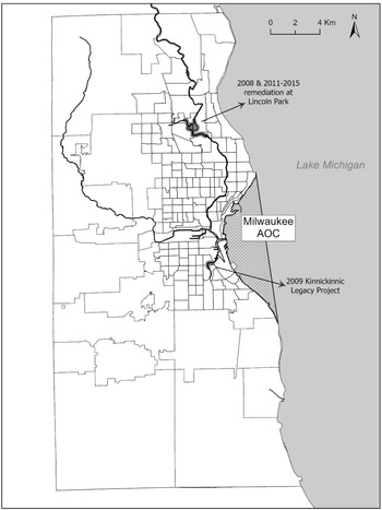
The Milwaukee Estuary AOC is located in Milwaukee, Wisconsin along the shore of Lake Michigan. Milwaukee is an urban and industrial center where municipal sewage, industrial waste, combined sewer overflow, and urban runoff contribute to water pollution (US EPA). The 2021 RAP progress report attributes seven BUIs in the AOC to contaminated sediments (Wisconsin Department of Natural Resources 2020). Studies since the 1970s have found high levels of PCBs in the Milwaukee River, which empties into Lake Michigan at the estuary and contributes to a large portion of the lake’s PCB contamination (Wethington and Hornbuckle Reference Wethington and Hornbuckle2005). Fish consumption advisories due to PCBs have been issued in the Milwaukee River since 1976 (Wisconsin Department of Natural Resources 2020). The original 1987 AOC boundaries included the harbor and nearshore area as well the lower portions of the Milwaukee, Menomonee, and Kinnikinnic Rivers, above their confluence in the city. The geographic boundaries were expanded in 2008 to include the upper portions of the rivers. Since that time, the WDNR and EPA have completed several remediation projects removing PCBs.
Public awareness of PCB concentrations in the water could have arisen as early as 1976 following the first fish advisories. Awareness likely increased when the Milwaukee Estuary was designated as an AOC in 1987 and with the expansion of the AOC’s boundaries to include the upper Milwaukee, Menominee, and Kinnickinnic Rivers in 2008. The expansion was specifically to address sources of contaminated sediment loads in the lower estuary (University of Wisconsin-Madison Division of Extension). The Wisconsin Department of Health Services (DHS) uses signage near the Milwaukee River to inform users about the conditions of the river and wildlife consumption advisories (Wisconsin Department of Natural Resources 2020).
This paper focuses on the effect of remediation actions that occurred between 2008 and 2015. The first action removed several hundred pounds of PCBs from the upper Milwaukee River at Lincoln Park in 2008. The second action removed 1,200 pounds of PCBs and 13,000 pounds of PAHs between Becher Street and KK Avenue on the Kinnickinnic River in 2009. This cleanup also made the river more navigable, by dredging the riverbed and removing objects and debris. The third and fourth actions removed contaminated sediments and restored wetland and riparian habitat in the upper Milwaukee River, upstream and downstream of Lincoln Park. The third action removed 5,028 pounds of PCBs and 4,035 pounds of PAHs in 2011 and 2012 (Wisconsin Department of Natural Resources & Office of the Great Lakes 2014), while the fourth action removed 2,330 pounds of PCBs and 12,683 pounds of PAHs in 2014 and 2015 (Environmental Quality Management 2016).
Economic research on Great Lakes AOCs
Previous research indicates that restoring AOCs provides economic benefits. Table 1 presents the list of papers on this topic and their study area, methodology, and results. Note that the table presents either one benefit estimate or a range of estimates from each paper and does not present a complete set of estimates, though we believe the values to be a fairly representative sample. The values range from $2,296 to $46,421 per household. As a percentage of house value, the range is 2% to 29%. These estimates imply that the value of restoring an AOC as a whole can range from a few million to several hundred million dollars. For example, McMillen (Reference McMillen2017) estimated that the aggregate benefit of restoring the Grand Calumet River AOC would be $5.92 million, and Braden et al. (Reference Braden, Won, Taylor, Mays, Cangelosi and Patunru2008b) estimated that the benefit of restoring the Sheboygan River AOC for homes within 5 miles would be either $158 million or $218 million, depending on whether one prefers estimates based on revealed or stated preference data.Footnote 1 Nearly all papers estimated benefits using property value hedonics, applied to either revealed or stated preference data, although sometimes both. However, Braden et al. (Reference Braden, Feng, L. Freitas and Won2010) used meta-analysis to estimate the benefits of restoring 23 U.S. AOCs, which they estimated would return $5.2 billion in lost residential property value.
Table 1. Prior economic research with selected estimates of willingness to pay to restore AOCs

* RP and SP indicate the authors used revealed preference and stated preference data, respectively.
Prior research has often found that the benefits of cleaning up are largest for households living closest to the water. McMillen (2006) estimated that restoring the Grand Calumet River AOC would increase values 27% for homes directly adjacent to the river and 18% for homes two and three blocks away. Braden et al. (Reference Braden, Taylor, Won, Mays, Cangelosi and Patunru2008a) estimated that restoring the Buffalo River AOC would increase home values within 1.5 miles of the AOC by 13%, and for homes within 5 miles of the AOC by 5%. Similarly, Braden et al. (Reference Braden, Won, Taylor, Mays, Cangelosi and Patunru2008b) estimated that restoring the Sheboygan River AOC would increase values by 12%–20% for homes immediately adjacent to the AOC and 3%–5% for homes 2 miles from the AOC.
Stoll et al. (Reference Stoll, Bishop and Keillor2002) and Melstrom (Reference Melstrom2022) are the only studies we are aware of that did not measure benefits within a hedonic framework. Stoll et al. (Reference Stoll, Bishop and Keillor2002) measured WTP directly using a survey with a referenda-style contingent valuation question based on removing the BUIs in the Lower Green Bay and Fox River AOC. Their research is important for two reasons: first, they examined whether WTP varies with the extent of cleanup, and, second, they compared differences in WTP between households living in and outside the vicinity of AOCs. They found diminishing marginal benefits as remediation increases from 20% to 100% of contaminated sediments. The estimates of partial to full remediation ranged from about $100 to $300 per household annually; their preferred estimate is $222 per household for 100% cleanup.Footnote 2 They also reported, based on responses to an open-ended follow-up question, that those adjacent to the AOC are willing to pay more for remediation than those living farther away. Melstrom (Reference Melstrom2022) used a residential sorting model to find that households in the Milwaukee Estuary AOC were willing to pay 29% of home value if they lived adjacent to cleanup and 12% of home value if they lived 1 mile from cleanup. Melstrom’s research contributes to questions about the distributional consequences of restoring AOCs because he does not find precise evidence that WTP varies between race and income groups, based on a time series cross section of home sales.
It should be pointed out that most prior research provides only partial information about the value of restoring AOCs. Prior research has largely focused on measuring use values, rather than both use and nonuse values. Nonusers can benefit from restoration because they may eventually use the water resource, or from simply knowing that the resource exists. Stoll et al. (Reference Stoll, Bishop and Keillor2002) are an exception because the effects of restoring the Green Bay AOC in their hypothetical remediation program were general rather than restricted to, for example, recreational activities. The distinction between use and nonuse is important because nonuse values can be substantial and prove to be a deciding factor in benefit-cost analysis (Loomis Reference Loomis2006; Kenney et al. Reference Kenney, Wilcock, Hobbs, Flores and Martínez2012). Thus, there is a pressing need for more research into restoring AOCs, such as Stoll et al. (Reference Stoll, Bishop and Keillor2002), that account for sources of cleanup value missed by most economic studies, and hedonic studies in particular.
Our research also captures only a portion of total restoration benefits in that we focus on a source of use value; however, our research design shines more light on the amount of this value. Most prior research has measured benefits based on individual home sales in a hedonic (e.g. Braden et al. Reference Braden, Taylor, Won, Mays, Cangelosi and Patunru2008a) or a sorting (e.g. Melstrom Reference Melstrom2022) framework, which provides insight into the values of owners but not renters. In contrast, our empirical strategy is based on geographically aggregated location decisions across demographic groups. Our research therefore shines new light on the use values of renters as well as owners. This is important because renters typically make up a large portion of households and environmental quality shocks can actually leave renters worse off, fostering environmental justice concerns (Melstrom et al. Reference Melstrom, Mohammadi, Schusler and Krings2022).
Methods
To look for evidence that households value restoring AOCs, we examine the location and move decisions of Milwaukee residents in response to remediation projects in the AOC between 2008 and 2015. We link location decisions to these projects using a two-stage sorting model. The /first stage consists of a system of equations that calculates the probability that a household in a neighborhood will move to another neighborhood. We separate households into six groups – including Black renters, Black owners, Hispanic renters, Hispanic owners, White renters, and White owners – to allow for tenure and race-specific differences in moves. We then use the system of equations to estimate the mean utility in a neighborhood for each group in 2000–2010 and 2010–2020. The idea behind modeling moves in these two decades is, if households value water quality improvements, then moves between 2010 and 2020, which occurred either during or after cleanup, should be significantly different than those between 2000 and 2010. The second stage measures the link between the value of residential locations, the AOC, and remediation by applying regression analysis to the mean utilities, expressed in terms of WTP, and proximity to the AOC.
Sorting model
The first stage of the sorting model simulates a household’s decision to move from location k to j. The decision is a function of the utility from living in each location, which can be written as
 $${U_{ikt}} = {\delta _{kt}} + {\eta _{ikt}}$$
which says household i’s utility from location k in decade t is equal to the mean utility ${\delta _{kt}}$
from the location and an idiosyncratic component
${\delta _{kt}}$
from the location and an idiosyncratic component ${\eta _{ikt}}$
unique to the household. The mean utility is a function of location attributes
${\eta _{ikt}}$
unique to the household. The mean utility is a function of location attributes ${X_{kt}}$
, the cost of housing
${X_{kt}}$
, the cost of housing ${P_{kt}}$
, unobservable attributes
${P_{kt}}$
, unobservable attributes ${\xi _{kt}}$
, and a vector of parameters
${\xi _{kt}}$
, and a vector of parameters ${\beta _t}$
,
${\beta _t}$
,
 $${\delta _{kt}} = f\left( {{X_{kt}},{P_{kt}},\;{\xi _{kt}};\;{\beta _t}} \right).$$
Following Depro et al. (Reference Depro, Timmins and O’Neil2015), we express the effect on utility of moving from k to j as
 $${U_{ijt}} - {U_{ikt}} = \left( {{\delta _{jt}} - {\delta _{kt}}} \right)\; - \;{\mu _t}M{C_{j,kt}} + ({\eta _{ijt}} - {\eta _{ikt}})$$
where $M{C_{j,kt}}$
is the cost of the move and
$M{C_{j,kt}}$
is the cost of the move and ${\mu _t}$
measures the marginal effect of moving cost on utility. When an individual does not move,
${\mu _t}$
measures the marginal effect of moving cost on utility. When an individual does not move, $M{C_{j,kt}}\;$
= 0. As we describe below,
$M{C_{j,kt}}\;$
= 0. As we describe below, ${\mu _t}$
is a parameter to be estimated that identifies the marginal utility of income, which we use to convert estimates of mean utility into WTP.
${\mu _t}$
is a parameter to be estimated that identifies the marginal utility of income, which we use to convert estimates of mean utility into WTP.
The probability of a move from k to j equals the share of residents that actually move from k to j, which we refer to as ${s_{j,k}}$
. Assuming that
${s_{j,k}}$
. Assuming that ${\eta _{ikt}}$
is i.i.d. Type I extreme value, then the share who move can be written as a logit that is a function of the difference in mean utilities and moving cost,
${\eta _{ikt}}$
is i.i.d. Type I extreme value, then the share who move can be written as a logit that is a function of the difference in mean utilities and moving cost,
 $${s_{j,kt}} = {{{e^{\left( {{\delta _{jt}} - {\delta _{kt}} - {\mu _t}M{C_{j,kt}}} \right)}}} \over {\mathop \sum \nolimits_{l = 1}^{N + 1} {e^{\left( {{\delta _{lt}} - {\delta _{kt}} - {\mu _t}M{C_{l,k}}} \right)}}\;}}.$$
where l is a location alternative and N+1 is the number of location alternatives in Milwaukee plus a catch-all location that accounts for moves to and from Milwaukee.
To estimate the mean utilities and the moving cost parameter, we set up a system of equations that predicts the share of households living in each location at the end of a decade using the observed populations at the start of the decade and equation (4). To see this, note that the population living in j in t+10 can be written as
 $$pop_j^{t + 10} = \;\mathop \sum \nolimits_{k = 1}^{N + 1} {s_{j,kt}}\;pop_k^t.$$
Dividing the equation above by the total population, $TOTPOP = \;\mathop \sum \nolimits_{k = 1}^{N + 1} \;pop_k^t = \;\mathop \sum \nolimits_{k = 1}^{N + 1} {s_{j,k}}\;pop_k^{t + 10}$
, we have
$TOTPOP = \;\mathop \sum \nolimits_{k = 1}^{N + 1} \;pop_k^t = \;\mathop \sum \nolimits_{k = 1}^{N + 1} {s_{j,k}}\;pop_k^{t + 10}$
, we have
 $$\sigma _j^{t + 10} = \mathop \sum \nolimits_{k = 1}^{N + 1} \left( {{{{e^{\left( {{\delta _{jt}} - {\delta _{kt}} - {\mu _t}M{C_{j,k}}} \right)}}} \over {\mathop \sum \nolimits_{l = 1}^N {e^{\left( {{\delta _{lt}} - {\delta _{kt}} - {\mu _t}M{C_{l,k}}} \right)}}}}} \right)\sigma _k^t.$$
which says the share living in j at the end of the decade, $\sigma _j^{t + 10}$
, is the sum of the shares moving to j from alternative locations k over the preceding decade, plus those who do not move away from j, multiplied by the population shares living in the locations at the start of the decade. We also include an equation for the percentage of Milwaukee population that did not move between t and t+10,
$\sigma _j^{t + 10}$
, is the sum of the shares moving to j from alternative locations k over the preceding decade, plus those who do not move away from j, multiplied by the population shares living in the locations at the start of the decade. We also include an equation for the percentage of Milwaukee population that did not move between t and t+10,
 $$\% Stay = \;{{\mathop \sum \nolimits_{k = 1}^N {s_{k,k}}pop_k^{t + 10}} \over {\mathop \sum \nolimits_{l = 1}^N pop_k^{t + 10}}}.$$
Using N+1 equations (6), which includes one equation for each location alternative, and equation (7), we have a system of N+2 equations to estimate the N+1 mean utilities ${\delta _{jt}}$
and the moving cost parameter
${\delta _{jt}}$
and the moving cost parameter ${\mu _t}$
.
${\mu _t}$
.
We solve for ${\delta _{jt}}$
and
${\delta _{jt}}$
and ${\mu _t}$
as follows: First, we fill in the
${\mu _t}$
as follows: First, we fill in the $pop_j^t$
using census tracts in the Milwaukee metropolitan area (i.e. Milwaukee County) as locations and group-specific tract populations from decennial census data. For the catch-all location, we follow Depro et al. (Reference Depro, Timmins and O’Neil2015) by setting the population to two times the absolute value of the difference between the group population in t and t+10 in Milwaukee. Second, we calculate the percentage of residents who do not move (i.e. those who stay) over the last decade using responses to the 2010 and 2019 American Community Survey. Third, we estimate move costs between all locations, expressed as an annualized cost; we describe calculating these costs below. Fourth, after normalizing one of the mean utilities to zero, we take an initial guess of
$pop_j^t$
using census tracts in the Milwaukee metropolitan area (i.e. Milwaukee County) as locations and group-specific tract populations from decennial census data. For the catch-all location, we follow Depro et al. (Reference Depro, Timmins and O’Neil2015) by setting the population to two times the absolute value of the difference between the group population in t and t+10 in Milwaukee. Second, we calculate the percentage of residents who do not move (i.e. those who stay) over the last decade using responses to the 2010 and 2019 American Community Survey. Third, we estimate move costs between all locations, expressed as an annualized cost; we describe calculating these costs below. Fourth, after normalizing one of the mean utilities to zero, we take an initial guess of ${\delta _{jt}}$
and
${\delta _{jt}}$
and ${\mu _t}$
, and then update the guess for
${\mu _t}$
, and then update the guess for ${\delta _{jt}}$
following the contraction mapping procedure described in Depro et al. (Reference Depro, Timmins and O’Neil2015) until
${\delta _{jt}}$
following the contraction mapping procedure described in Depro et al. (Reference Depro, Timmins and O’Neil2015) until $\left| {\delta _{jt}^{m + 1} - \delta _{jt}^m} \right| \lt {10^{ - 7}}\;\forall \;j$
, where m counts the number of updates after the initial guess. We use the bisection method to search over the values of
$\left| {\delta _{jt}^{m + 1} - \delta _{jt}^m} \right| \lt {10^{ - 7}}\;\forall \;j$
, where m counts the number of updates after the initial guess. We use the bisection method to search over the values of ${\mu _t}$
that match the predicted and actual
${\mu _t}$
that match the predicted and actual $\% stay$
, re-solving for the
$\% stay$
, re-solving for the ${\delta _{jt}}$
s at each step. We follow this procedure twice for each group, first using 2000–2010 data and second using 2010–2020 data.
${\delta _{jt}}$
s at each step. We follow this procedure twice for each group, first using 2000–2010 data and second using 2010–2020 data.
Partial aggregation of the location alternatives
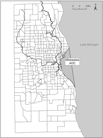
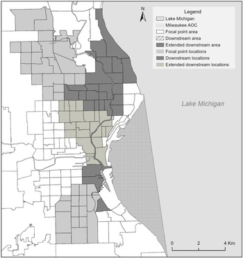
We combine several of the tracts into grouped alternatives to address changing boundaries and reduce the computational burden of estimation. Census tract boundaries can change from census to census, so to define location alternatives with stable boundaries, we group tracts that were split or combined between 2000, 2010, and 2020. For example, to account for the fact that tract 1 was split into 1.01 and 1.02 after 2000, we combine the demographics of 1.01 and 1.02 into a single location in 2010 and 2020. This procedure produces 13 aggregated locations. Next, we group tracts farther than four kilometers from the AOC into aggregated locations. Figure 1 shows the 2020 tract boundaries while Figure 2 shows the aggregated locations. We do not expect this procedure to create bias (i.e. as a result of the ecological fallacy; see Banzhaf and Walsh (Reference Banzhaf and Walsh2008)) because the boundaries of these aggregated locations align closely with the boundaries of relatively homogenous suburbs, which are unlikely to be affected by distant water quality improvements. Research finds that partially aggregated choice models that leave the alternatives of primary interest disaggregated can approximate the results of fully disaggregated models, as long as one includes the term $\ln \left( {{M_i}} \right)$
in the regression, where
$\ln \left( {{M_i}} \right)$
in the regression, where ${M_i}$
is the number of elemental alternatives (tracts) in each alternative (Lupi and Feather Reference Lupi and Feather1998), as we do here. Including the catch-all, this aggregation process produces a choice set of 154 locations.
${M_i}$
is the number of elemental alternatives (tracts) in each alternative (Lupi and Feather Reference Lupi and Feather1998), as we do here. Including the catch-all, this aggregation process produces a choice set of 154 locations.

Figure 1. The Milwaukee Estuary AOC and census tracts in the Milwaukee metropolitan area.

Figure 2. Restoration actions in the Milwaukee Estuary AOC and the residential locations used in the study.
Regression analysis
We estimate WTP in the second stage by applying regression to the estimates of ${\delta _{jt}}$
and
${\delta _{jt}}$
and ${\mu _t}$
produced in the first stage. Let
${\mu _t}$
produced in the first stage. Let $\delta _{jt}^g$
and
$\delta _{jt}^g$
and $\mu _t^g$
refer to the mean utilities and the move cost parameter (marginal utility of income) in decade t for each demographic group g. To convert the mean utilities into comparable dollar values, we divide
$\mu _t^g$
refer to the mean utilities and the move cost parameter (marginal utility of income) in decade t for each demographic group g. To convert the mean utilities into comparable dollar values, we divide $\delta _{jt}^g$
by
$\delta _{jt}^g$
by $\mu _t^g$
. Now, consider the regression of
$\mu _t^g$
. Now, consider the regression of $\delta _{jt}^g/\mu _t^g$
on
$\delta _{jt}^g/\mu _t^g$
on ${X_{jt}}$
,
${X_{jt}}$
, ${P_{jt}}$
,
${P_{jt}}$
, ${\rm{ln}}\left( {{M_j}} \right)$
and
${\rm{ln}}\left( {{M_j}} \right)$
and $\xi _{jt}^g$
:
$\xi _{jt}^g$
:
 $${{\;\delta _{jt}^g} \over {\mu _t^g}} = \tilde \beta _X^g{X_{jt}} + \tilde \beta _P^g{P_{jt}} + {{{\rm{ln}}\left( {{M_j}} \right)} \over {\mu _t^g}} + {{\xi _{jt}^g} \over {\mu _t^g}}.$$
where a tilde indicates that $\beta $
is divided by the move cost parameter, that is,
$\beta $
is divided by the move cost parameter, that is, $\tilde \beta _l^g = \beta _l^g/\mu _t^g$
for l = X, P. In the regression,
$\tilde \beta _l^g = \beta _l^g/\mu _t^g$
for l = X, P. In the regression, ${X_{jt}}$
includes location attributes important to households including neighborhood demographics, proximity to the AOC, and any remediation actions.
${X_{jt}}$
includes location attributes important to households including neighborhood demographics, proximity to the AOC, and any remediation actions.
We estimate a modified version of equation (8). First, we fix $\tilde \beta _P^g = - 1$
because in theory utility measured in dollars should decrease by one dollar when the price of housing increases by a dollar. Second, we move
$\tilde \beta _P^g = - 1$
because in theory utility measured in dollars should decrease by one dollar when the price of housing increases by a dollar. Second, we move ${P_{jt}}$
to the left-hand side. Next, to account for the panel nature of our data, we include the variable
${P_{jt}}$
to the left-hand side. Next, to account for the panel nature of our data, we include the variable $pos{t_{jt}}$
, which equals one if the mean utility occurs in the 2010–2020 decade. We then separate
$pos{t_{jt}}$
, which equals one if the mean utility occurs in the 2010–2020 decade. We then separate ${X_{jt}}$
between variables measuring proximity to the AOC and other attributes
${X_{jt}}$
between variables measuring proximity to the AOC and other attributes ${Z_{jt}}$
. We measure proximity using the gravity index
${Z_{jt}}$
. We measure proximity using the gravity index $1/{d_j}$
, where
$1/{d_j}$
, where ${d_j}$
is the distance in kilometers from the centroid of a location to the nearest point on the AOC. This index allows the AOC to have a larger effect on utility in near than far locations, consistent with prior research (McMillen 2006; Braden et al. Reference Braden, Taylor, Won, Mays, Cangelosi and Patunru2008a). Finally, to account for the effect of the four remediation projects between 2008 and 2015, let
${d_j}$
is the distance in kilometers from the centroid of a location to the nearest point on the AOC. This index allows the AOC to have a larger effect on utility in near than far locations, consistent with prior research (McMillen 2006; Braden et al. Reference Braden, Taylor, Won, Mays, Cangelosi and Patunru2008a). Finally, to account for the effect of the four remediation projects between 2008 and 2015, let $cleanu{p_{jt}}$
equal one for locations whose closest point to the AOC was affected by remediation. We then estimate the following equation:
$cleanu{p_{jt}}$
equal one for locations whose closest point to the AOC was affected by remediation. We then estimate the following equation:
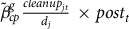
 $$\matrix{
{{P_{jt}} + {{\;\delta _{jt}^g} \over {\mu _t^g}} = \tilde \beta _p^gpos{t_t} + \tilde \beta _d^g{1 \over {{d_j}}} + \tilde \beta _c^g{{cleanu{p_{jt}}} \over {{d_j}}} + \tilde \beta _{cp}^g{{cleanu{p_{jt}}} \over {{d_j}}} \times pos{t_t} + \tilde \beta _Z^g{Z_{jt}} + {{{\rm{ln}}\left( {{M_j}} \right)} \over {\mu _t^g}}} \hfill \cr
{\quad \quad \quad \quad + {{\xi _{jt}^g} \over {\mu _t^g}}.} \hfill \cr } $$
$$\matrix{
{{P_{jt}} + {{\;\delta _{jt}^g} \over {\mu _t^g}} = \tilde \beta _p^gpos{t_t} + \tilde \beta _d^g{1 \over {{d_j}}} + \tilde \beta _c^g{{cleanu{p_{jt}}} \over {{d_j}}} + \tilde \beta _{cp}^g{{cleanu{p_{jt}}} \over {{d_j}}} \times pos{t_t} + \tilde \beta _Z^g{Z_{jt}} + {{{\rm{ln}}\left( {{M_j}} \right)} \over {\mu _t^g}}} \hfill \cr
{\quad \quad \quad \quad + {{\xi _{jt}^g} \over {\mu _t^g}}.} \hfill \cr } $$
where $\tilde \beta _d^g{1 \over {{d_j}}}$
measures the effect of AOC proximity on the desirability of living in location j, and
$\tilde \beta _d^g{1 \over {{d_j}}}$
measures the effect of AOC proximity on the desirability of living in location j, and $\tilde \beta _c^g{{cleanu{p_{jt}}} \over {{d_j}}}$
measures any difference in the proximity effect between locations near the remediation area and those nearer other points on the AOC. If households dislike living close to the AOC, as prior research suggests, then
$\tilde \beta _c^g{{cleanu{p_{jt}}} \over {{d_j}}}$
measures any difference in the proximity effect between locations near the remediation area and those nearer other points on the AOC. If households dislike living close to the AOC, as prior research suggests, then $\tilde \beta _d^g$
will be negative. The term
$\tilde \beta _d^g$
will be negative. The term $\tilde \beta _{cp}^g{{cleanu{p_{jt}}} \over {{d_j}}} \times pos{t_t}$
measures the change in the proximity effect caused by remediation. If, other things equal, households prefer living near restored water conditions, then
$\tilde \beta _{cp}^g{{cleanu{p_{jt}}} \over {{d_j}}} \times pos{t_t}$
measures the change in the proximity effect caused by remediation. If, other things equal, households prefer living near restored water conditions, then $\tilde \beta _{cp}^g$
will be positive.
$\tilde \beta _{cp}^g$
will be positive.
To account for group-level differences, we estimate equation (9) using the following functional form for $\beta _l^g$
, where l = d, c, cp, Z:
$\beta _l^g$
, where l = d, c, cp, Z:
 $$\beta _l^g = \beta _{l,0}^{} + \sum \beta _{l,k}^{}{z_k}$$
where $\beta _{l,0}^{}$
measures the effect on the base group and
$\beta _{l,0}^{}$
measures the effect on the base group and $\beta _{l,k}^{}{z_k}$
measures the effect in group k relative to the base group. We define the base group as White owners and
$\beta _{l,k}^{}{z_k}$
measures the effect in group k relative to the base group. We define the base group as White owners and ${z_k}$
as an indicator for k = renter, Black and Hispanic. Expressed this way,
${z_k}$
as an indicator for k = renter, Black and Hispanic. Expressed this way, $\beta _{l,k}^{}{z_k}$
measures any WTP disparity or premium for households that belong to a historically marginalized group.
$\beta _{l,k}^{}{z_k}$
measures any WTP disparity or premium for households that belong to a historically marginalized group.
The extent that the four remediation projects reduced PCB concentrations and improved downstream water quality is unknown, so we explore several different area definitions of $cleanu{p_{jt}}$
. The first definition, which we refer to as the focal point area, includes only the locations whose nearest point on the AOC had contaminated sediments removed. This includes one mile of the Milwaukee River at Lincoln Park and one half-mile of the Kinnickinnic River. The second definition, which we refer to as the downstream area, includes locations nearest the upper (but not the lower) Milwaukee River running from Lincoln Park and the Humboldt Avenue Bridge, and locations nearest the Kinnickinnic River running from Becher Street to the confluence with the Milwaukee River. The third definition, which we refer to as the extended downstream area, covers the previous definition plus the lower Milwaukee River, which includes the remaining downstream portion above Lake Michigan. See Figure 3 for a map of these areas. Comparing results across these definitions allows us to empirically assess the geographic extent that households responded to the remediation projects.
$cleanu{p_{jt}}$
. The first definition, which we refer to as the focal point area, includes only the locations whose nearest point on the AOC had contaminated sediments removed. This includes one mile of the Milwaukee River at Lincoln Park and one half-mile of the Kinnickinnic River. The second definition, which we refer to as the downstream area, includes locations nearest the upper (but not the lower) Milwaukee River running from Lincoln Park and the Humboldt Avenue Bridge, and locations nearest the Kinnickinnic River running from Becher Street to the confluence with the Milwaukee River. The third definition, which we refer to as the extended downstream area, covers the previous definition plus the lower Milwaukee River, which includes the remaining downstream portion above Lake Michigan. See Figure 3 for a map of these areas. Comparing results across these definitions allows us to empirically assess the geographic extent that households responded to the remediation projects.

Figure 3. The treated area definitions used in the study.
Data
The primary data set in the first stage comes from the U.S. Census Bureau’s tract-level cross-tabulations from the 2000 and 2010 decennial censuses and the 2020 5-year American Community Survey (ACS), which we use to measure tract populations for each demographic group.Footnote 3 We then turn to 1-year ACS microdata to construct the metro-area stay percentages for each group. Table 2 provides summaries of these data.
Table 2. Data used in the Milwaukee residential sorting model

Panel A presents the first-stage data from the U.S. Census Bureau’s tract-level cross-tabulations from the 2000 and 2010 decennial censuses and 2020 5-year American Community Survey (ACS). Panel B presents the second-stage data from the decennial censuses for data from 2000 and 2010. Median home values and rents for 2005 and 2015 are from 5-year ACS data. 2005 rent and home value are the average of 2000 and 2010 ACS values because data from the year 2005 were not available. All dollar values have been adjusted to 2020$ values.
The first stage also requires moving costs, which we measure as the sum of the physical, financial and search costs of moving in 2000–2010 and 2010–2020. We calculate these costs separately for owners and renters to account for differences in spending and move frequency. For physical moving costs, we use $2,033 for owners, which is the midpoint of the range provided by moving.com to move a three-bedroom household in Milwaukee County. We use $1,323.50 for renters, which is the midpoint provided by moving.com to move a two-bedroom household. Next, we add the time value of moving. We assume two adult packs and unpack for four hours each and then travel from the origin location to the destination location at a speed of forty-five miles per hour. This assumption does not have a large effect on our results; in an appendix, we show that results are similar if we use a higher time value, based on a driving speed of fifteen miles per hour. We assume a time value of $23.30 and $25.58, based on the median wage in Milwaukee in 2005 and 2015, respectively. The sum of all of these values is the total physical costs for owners and renters. For moves to and from the catch-all location, we assume a fixed physical moving cost of $5,000 for owners and $4,000 for renters (Bieri et al. Reference Bieri, Kuminoff and Pope2014).
For financial costs, we use data on the median home value and rent in each tract. For 2000–2010 moves, we use the average of median home values and rents reported by the Census in 2000 and 2010. For the 2010–2020 moves, we use median home values and rents reported in 2015. For the catch-all location, we assume a home value of $149,750 and rent of $728.50 in 2005, and a home value of $194,500 and rent of $959 in 2015, which are the median U.S. values in those years. We assume homeowners pay 3.5% of median home value in both the original location and new location, which includes a 6% realtor commission split between the buyer and seller and 1% closing costs. For renters, we assume financial costs are half of the median rent in a location, which represents a non-refundable deposit. Finally, we assume a search cost for a new residence of $20 per mile, based on the distance between the old and new location. Our results are largely insensitive to modest variations in this cost; in the appendix, we show that replacing it with a fixed $500 or dropping it altogether has little effect on the estimates.
We sum the physical, financial, and search costs for owners and renters, and then annualize these sums using a 5% discount rate and a time horizon of eight years for owners and two years for renters (Melstrom et al. Reference Melstrom, Mohammadi, Schusler and Krings2022), which represent the time owners and renters typically reside in a home before relocating. We go through these calculations twice, first for the 2000–2010 moves and second for the 2010–2020 moves. We adjust moving costs to 2020$ using the consumer price index.
For the second stage, we collect tract-level data on educational attainment, income, location demographics, and geographic features. The 2000 and 2010 Decennial Censuses are sources for the percent of people over 25 years old with a bachelor’s degree, median household income, and percentages of Black, White, and Hispanic residents. Geographic features include proximity to Lake Michigan, nearest freeway, Superfund sites, and the AOC. Proximity to Lake Michigan, nearest freeway, and Superfund sites are simply dummy variables equal to one if a tract has shoreline on Lake Michigan, has a freeway running through it, or is located within one kilometer of a Superfund site. We measure proximity to the AOC using the gravity index based on the distance between a tract and the closest part of the AOC.
Before turning to the results, we should note that, depending on the group and decade, the populations of some locations are zero. In total, 15.9% of locations have no Black owners, 2.9% of locations have no Black renters, 14.6% have no Hispanic owners, 4.9% have no Hispanic renters, 5.8% have no White owners, and 3.6% have no White renters. This makes identifying the group and decade-specific mean utilities in these locations challenging, because first-stage estimation cannot determine how desirable or undesirable these locations are. It is also possible that these locations have zero population because they are inaccessible or omitted from a groups’ choice set. Our solution is to simply exclude these group and decade-specific mean utilities from second-stage estimation. The appendix includes results if we instead calculate these mean utilities by “patching” the zeros with a small, artificial population of 0.1.
Results
First-stage estimates
The first stage produces 1,668 mean utilities and moving cost parameters when we exclude the group-decade-location combinations with a population of zero. The moving cost parameters reported in Table 3 show that, across most groups, the effect of moving cost declined between 2000–2010 and 2010–2020. This could be due to rising average incomes or a change in tastes about moving (see Table 2).
Table 3. Moving costs parameter (marginal utility of income) estimates from the first stage of the model

Second-stage estimates
The model coefficients associated with AOC proximity and cleanup are shown in Table 4. The complete set of model coefficients is available in the appendix. The first column lists the proximity measures and the interactions for renters, Black households and Hispanic households. The second column shows the coefficient estimates when we assume remediation only affects locations in the focal point area, that is, where contaminated sediments were removed. The third and fourth columns show the results when we allow the effect to occur in the downstream area and extended downstream area, respectively. Recall that the coefficients can be interpreted as the marginal WTP per year for an attribute.
Table 4. AOC proximity effects estimated in the second stage of the model for three different areas that could have been affected by remediation
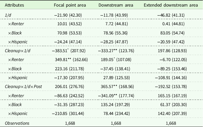
*and **indicate significantly different from zero at the 10% and 5% levels, respectively.
The results provide evidence that remediation affects location choice and WTP in the downstream area, rather than the focal point or extended downstream areas. The coefficient on the gravity index 1/d is not significantly different from zero in any of the three columns, so we cannot say whether White owners (the base group) prefer to live near the AOC or not before remediation. The insignificant coefficients on the demographic interactions provide little evidence that the mobility patterns of renters, Black or Hispanic households are different from White owners with respect to AOC proximity. This could be because most households value the esthetics of living near the water about as much as they dislike the BUIs. In the second and third columns, the coefficient on cleanup×1/d indicates that owner WTP is significantly lower to live near the focal point and downstream areas relative to other parts of the AOC. The demographic interactions provide no evidence Black or Hispanic WTP is different than White WTP; however, there is evidence of a difference between renter and owner WTP. These results imply that renters are significantly more likely to live near the focal point and downstream areas relative to owners, prior to cleanup. Turning to the variables of primary interest – cleanup×1/d×post and the interactions with renter, Black and Hispanic – none of coefficients are significant in the second column. In the third column, the coefficient on cleanup×1/d×post is significantly positive, and the interaction with renter is significantly negative. This indicates that WTP to live in the downstream area increased after the remediation projects for owners more than it did for renters. Finally, in the fourth column the coefficient on cleanup×1/d×post is not significantly different from zero.Footnote 4
Table 5 presents the change in group-specific WTP to live in the downstream area after remediation, using the average gravity index and the estimates in the third column of Table 4. Owner WTP for remediation is positive with small and insignificant differences between race groups. Renter WTP is also positive, though not significantly so. Average WTP is $268.08 (90% CI of 90.29 to 722.78) per year across all groups located near the downstream area. Averaging this across all households in Milwaukee County, including those not located near the cleanups, per-household WTP is $45 per year. Given confidence interval sizes, it is important not to take this or the group-specific WTP estimates at face value. Nevertheless, based on Table 5, the difference between owner and renter WTP – $384 – is large enough that it deserves attention. The differences between race group WTP – $152 more for Black households and $88 more for Hispanic households, relative to Whites – appear modest by comparison, though actual racial WTP disparities could be quite a bit smaller or larger than these estimates. So, while the estimates in Table 5 provide strong evidence that remediation increased WTP and hence affected decisions to live near the AOC for some if not most demographic groups, there is also evidence that the value of remediation was greater for owners than for renters.
Table 5. Group-specific increase in annual willingness to pay to live in downstream area after remediation
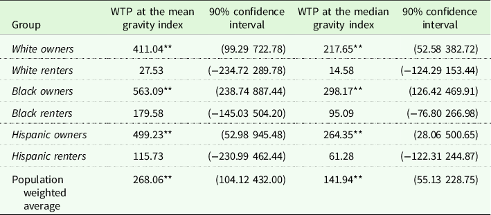
*and **indicate significantly different from zero at the 10% and 5% levels, respectively.
Table 5 also presents WTP estimates using the median gravity index. Locations adjacent to the AOC have very high gravity indexes that skew the average to the right of the median – 1.12 vs 0.60 – so WTP at the median may better reflect a typical household’s WTP in the downstream area. Comparing the two sets of estimates makes clear that the lower the gravity index – that is, the farther a location is from the AOC – the lower is WTP.
We can use these results to estimate the benefits of the remediation projects in the Milwaukee and Kinnickinnic Rivers. Multiplying the group-specific average WTP in Table 5 by the number of households living near the downstream area, the annual benefits of cleanup in each group are $5.18 million for White owners, $3.35 thousand for White renters, $5.37 million for Black owners, $3.12 million for Black renters, $1.85 million for Hispanic owners, and $769 thousand for Hispanic renters. Adding these benefits together and assuming other race-tenure groups (e.g. Asian and Native American), WTP equals the average in Table 5, and using a 5% discount rate, the present value aggregate benefits are $349.52 million. The total cost of remediation is $81.62 million: the 2008 remediation at Lincoln Park cost $1.59 million, while Phase 1 and Phase 2 of the 2011–2015 remediation at Lincoln Park cost $31.78 million and $20.88 million, respectively; and the 2009 Kinnickinnic Legacy Project cost $27.37 million.Footnote 5 The benefit-cost ratio of remediation is therefore about four, with a net benefit of $251 million.
These estimates are comparable with prior research on the benefits of cleaning up AOCs. Depending on how close a household lives, the effect of cleanup on WTP per household ranges from a few thousand dollars to more than $40,000 in the literature. Using a discount rate of 5%, our average WTP per-year estimate indicates that total WTP per household is $5,362 in the affected area. McMillen (2006) and Isely et al. (Reference Isely, Isely, Hause and Steinman2018) report similar values in restoring the Grand Calumet and Muskegon Lake AOCs, both of which are on Lake Michigan, similar to the Milwaukee Estuary AOC. Our value is lower than the per-household WTP estimates reported in Melstrom (Reference Melstrom2022) for Milwaukee; however, Melstrom focuses on owners, while our estimate includes the experiences of renters, which make up 59% of households in the city.Footnote 6
It is important to keep in mind that these WTP estimates only include benefits through home purchases, although there are many potential sources of benefits from AOC remediation, including values from non-residents. Thus, our benefit-cost ratio may severely underestimate the benefit of cleaning up the AOC. Nevertheless, our estimated aggregate WTP of $350 million does align with prior research on AOCs, which reports aggregate benefits ranging from $5.92 million to $875 million.
How sensitive are the estimates to changes in modeling assumptions? To help answer this question, we ran several additional regressions after revising either the set-up in the first stage or the specification in the second stage. One potential concern is that the large difference in renter and owner WTP could be driven by differences in renter and owner moving costs rather than by differences in moving behavior. We explore this issue by running the model again after equating renter and owner moving costs, using a weighted average of the renter and owner costs, similar to Depro et al. (Reference Depro, Timmins and O’Neil2015). These results are reported in Table 6. Focusing on the estimates for the downstream area in column three, the coefficient of cleanup×1/d×post is now slightly lower (365.57 vs 353.22), while the coefficient of cleanup×1/d×post×renter is slightly higher in absolute value (−341.09 vs. −335.31). These differences do not appear large enough to suggest that the disparity in WTP between renters and owners is due to assumptions about moving costs.
Table 6. AOC proximity effects when the model uses the same moving cost for owners and renters

Standard errors in parentheses below coefficients. *and **indicate significance at the 10% and 5% levels, respectively.
Another potential concern is that unobservables correlated with the location and timing of remediation actions could bias the parameters of interest. The AOC is located near the core of the metropolitan area, so perhaps the cleanup benefits estimated above are simply due to improvements in school quality, reductions in crime, etc. near the downtown area. To address this concern, we ran the regressions including a set of municipal fixed effects to control for city-specific (i.e. the city of Milwaukee and surrounding communities) unobservables, which are reported in Table 7. Focusing on the estimates for the downstream area in column three, we once again see that the coefficient of cleanup×1/d×post is positive and significant. The estimate on cleanup×1/d×post×renter also changes little, remaining negative and significant, while the other interaction effects are essentially unchanged. This suggests that the results are not biased due to municipal-level, correlated unobservables. We also estimated the second stage with tract fixed effects (results not shown but available upon request). Although the magnitudes of the 1/d and cleanup×1/d coefficients appear sensitive to controlling for tract-level unobservables, the sign and significance level of the cleanup×1/d×post coefficient is unchanged; the same is true for the interaction effects.
Table 7 AOC proximity effects when the second stage includes municipality fixed effects

Standard errors in parentheses below coefficients. *and **indicate significance at the 10% and 5% levels, respectively.
Four analyses probing the sensitivity of the estimates to modeling assumptions in the first stage can be found in the appendix. Many assumptions factor into our moving cost calculations, but our results appear robust. We also examined replacing zeros with 0.1 in tracts with group-specific populations of zero, which had little effect on White WTP but produced lower Black and Hispanic WTP.
Conclusion
Using a residential sorting model to simulate the moving behavior of households before and after several remediation projects in the Milwaukee Estuary AOC, we found WTP increased significantly to live near parts of the Milwaukee and Kinnikinnic Rivers after remediation. WTP scaled with distance from the AOC, so benefits appear to be concentrated around households that live near the water, particularly those downstream of where remediation took place. This proximity effect is consistent with prior research on AOCs (e.g. Braden et al. Reference Braden, Taylor, Won, Mays, Cangelosi and Patunru2008a; Isely et al. Reference Isely, Isely, Hause and Steinman2018). Benefits appear to attenuate as one moves downstream, though, because we found no evidence that demand and WTP increased when we allowed the affected area to include in the lowest part of the estuary. This does not mean that residents in this part of Milwaukee did not benefit from remediation, but it may suggest that at a far enough distance, residents do not take upstream water quality into account when deciding where to locate. There are many potential sources of benefits from water quality restoration besides improved property values that our analysis does not include, so our results necessarily underestimate of the value of remediation in the AOC. Additionally, only one of the eleven BUIs has been restored, and full cleanup may result in more benefits for Milwaukee residents.
We did not find any significant differences in WTP between race groups, although we did find an important difference between tenure groups. Owner WTP for cleanup appears much larger than renter WTP, by up to several hundred dollars per year, for the remediation projects that have occurred in the AOC since 2008. This suggests that cleanup disproportionately benefited owners. The lack of significant WTP disparities between race groups is consistent with prior research (Melstrom Reference Melstrom2022). This is important because improvements in environmental quality have the potential to drive out low-income and minority groups due to income disparities or discrimination. While all households may benefit from neighborhood improvements, changes that benefit (i.e. are associated with a larger WTP) some groups more than others can contribute to demographic turnover. The results in this paper suggest that owners have disproportionately moved into neighborhoods affected by remediation. This outcome lends support for claims in the environmental justice literature that working-class households – who are disproportionately renters – are least likely to benefit from environmental improvements due to competition and discrimination in the housing market. Restoring AOCs may be desirable for most households, but conditions in areas like Milwaukee allow homeowners to benefit the most from remediation.
Supplementary material
To view supplementary material for this article, please visit https://doi.org/10.1017/age.2023.10
Data availability statement
The data that support the findings of this study are available from the corresponding author.
Funding statement
Donnelly and Melstrom declare none.
Competing interests
Donnelly and Melstrom declare none.


 Open access