


1. Introduction
Transition to turbulence in wall-bounded shear flows is a classical problem of both fundamental and practical interest, which, however, has not yet been fully understood. The current state of knowledge can be found in recent reviews (Pomeau Reference Pomeau2015; Barkley Reference Barkley2016; Manneville Reference Manneville2017; Eckhardt Reference Eckhardt2018; Tuckerman, Chantry & Barkley Reference Tuckerman, Chantry and Barkley2020). Here, we experimentally investigate the transitional range of Reynolds numbers in plane Couette–Poiseuille flow, an example of a shear flow, which has received little attention up to now (see Klotz et al. (Reference Klotz, Lemoult, Frontczak, Tuckerman and Wesfreid2017) and references therein). Specifically, the Couette–Poiseuille velocity profile with zero-mean advection velocity (similar to our case) was investigated by Huey & Williamson (Reference Huey and Williamson1974) and Tsanis & Leutheusser (Reference Tsanis and Leutheusser1988), who concentrated mainly on fully developed turbulence. In addition, Tsanis & Leutheusser (Reference Tsanis and Leutheusser1988) stated that the transition from the laminar to the turbulent state occurs at  $Re\approx 900$, but without discussing this result.
In this context Klotz & Wesfreid (Reference Klotz and Wesfreid2017) reported the first and detailed measurements of the response of shear flow to an impulsive well-controlled perturbation that triggers localized turbulent spots. Two possible types of evolution were observed. The first is characterized by an initial growth of a localized spot, which is eventually followed by an exponential decay. This type of evolution was quantitatively compared with linear transient growth theory (see also Schmid & Henningson Reference Schmid and Henningson2001) calculated for plane Couette–Poiseuille flow. The second type of behaviour corresponds to a self-sustained turbulent spot with postponed decay that results in a non-deterministic lifetime. However, in either of these two different behaviours, localized spots can eventually decay. We call the second type of evolution ‘self-sustained’ because streaks within the turbulent spot show non-trivial and nonlinear behaviour (including waviness of the streaks), which is similar to a self-sustained cycle described by Waleffe (Reference Waleffe1997) and experimentally observed by Duriez, Aider & Wesfreid (Reference Duriez, Aider and Wesfreid2009); see also the recent work of Dessup et al. (Reference Dessup, Tuckerman, Wesfreid, Barkley and Willis2018) for an analogous process in Taylor–Couette flow.
However, we recall that Waleffe's original model can describe only the temporal dynamics of a local turbulent structure (temporal aspect of transition to turbulence). Results obtained in long pressure-driven pipes in the transitional range of Reynolds numbers demonstrated that the characteristic lifetime of a single turbulent spot (called a puff) increases exponentially or even superexponentially (Hof et al. Reference Hof, de Lozar, Kuik and Westerweel2008; Avila, Willis & Hof Reference Avila, Willis and Hof2010; Kuik, Poelma & Westerweel Reference Kuik, Poelma and Westerweel2010; Mukund & Hof Reference Mukund and Hof2018) as the Reynolds number is increased, which implies that a single puff is a transient structure with finite characteristic lifetime. An explanation for truly self-sustained turbulence for an asymptotically large time horizon in the transitional range of Reynolds numbers requires one also to take into account the spatial aspect of the transition to turbulence (Pomeau Reference Pomeau1986). This point has been further elucidated by Manneville (Reference Manneville2009), who showed that the transformation from local temporal chaos to global sustained spatiotemporal chaos occurs independently of whether the lifetime of the local structures diverges or not.
Based on the single-puff statistics in pipe flow, Avila et al. (Reference Avila, Moxey, de Lozar, Avila, Barkley and Hof2011) proposed that an asymptotically self-sustained turbulence can be reached at a Reynolds number at which the puff decay is compensated by puff splitting (representing a spatial proliferation of the turbulent phase into the laminar flow). Recently, Mukund & Hof (Reference Mukund and Hof2018) generalized this argument based on single-puff statistics to the case of fully intermittent flow, in which several puffs can mutually interact. In addition, Lemoult et al. (Reference Lemoult, Shi, Avila, Jalikop, Avila and Hof2016) reported for one-dimensional Couette flow that, in the vicinity of the threshold of asymptotically self-sustained turbulence, a turbulent phase follows a continuous phase transition and can be described by the directed percolation statistical model. Chantry, Tuckerman & Barkley (Reference Chantry, Tuckerman and Barkley2017) observed similar critical behaviour in the domain extended in the two wall-parallel dimensions using a simplified model of shear flow reduced to only four modes along the wall-normal direction.
One important spatial aspect of the transition to turbulence in wall-bounded shear flows is the existence of large-scale flow induced around turbulent structures. This large-scale flow is related to the flow generated by the Reynolds stresses induced by nonlinearity of the Navier–Stokes equation, as postulated by Hayot & Pomeau (Reference Hayot and Pomeau1994). The modification of the laminar flow around a turbulent spot was observed by Henningson & Alfredsson (Reference Henningson and Alfredsson1987), Henningson (Reference Henningson1989), Henningson & Kim (Reference Henningson and Kim1991), Lundbladh & Johansson (Reference Lundbladh and Johansson1991) and Tillmark (Reference Tillmark1995). However, at the time, the main attention was focused on the linear stability of the modified laminar flow (Henningson & Alfredsson Reference Henningson and Alfredsson1987), which possibly might explain the spanwise growth of the turbulent spot (called growth by destabilization by Gad-El-Hak, Blackwelderf & Riley (Reference Gad-El-Hak, Blackwelderf and Riley1981) and Riley & Gad-El-Hak (Reference Riley and Gad-El-Hak1985)).
It is now known that the large-scale flow generated around a localized spot has a quadrupole topology and extends far into the laminar region (Schumacher & Eckhardt Reference Schumacher and Eckhardt2001; Lagha & Manneville Reference Lagha and Manneville2007; Duguet & Schlatter Reference Duguet and Schlatter2013; Brand & Gibson Reference Brand and Gibson2014; Wang et al. Reference Wang, Guet, Monchaux, Duguet and Eckhardt2020). For plane Couette flow, it has been demonstrated that the front between the laminar and turbulent regions is oblique along the wall-normal direction, where nearly laminar flow near one wall faces locally turbulent flow on the opposite wall (Coles Reference Coles1965; Lundbladh & Johansson Reference Lundbladh and Johansson1991; Barkley & Tuckerman Reference Barkley and Tuckerman2007; Duguet & Schlatter Reference Duguet and Schlatter2013). These are overhang regions, where the streamwise velocity profile averaged over the wall-normal direction is non-zero. For a localized turbulent spot, these regions lead to streamwise flow through upstream and downstream fronts towards the spot (Rolland Reference Rolland2014). Furthermore, measurements in boundary layer flow established that the wall pressure within the turbulent spot is lower than that in the laminar region at some distance upstream and downstream (Mautner & Van Atta Reference Mautner and Van Atta1982). By assuming scale separation between the large and small scales of the shear flow, the incompressibility of both scales can be considered independently (Duguet & Schlatter Reference Duguet and Schlatter2013). The incompressibility of the large scales implies that the streamwise flow through the laminar–turbulent interface towards the spot must be accompanied by a spanwise velocity component from the spot. This flow topology induces the quadrupolar large-scale flow.
The first experimental evidence of quadrupolar large-scale flow in shear flows was reported for plane Poiseuille flow by Lemoult, Aider & Wesfreid (Reference Lemoult, Aider and Wesfreid2013) and its full inclined three-dimensional structure was measured by Lemoult et al. (Reference Lemoult, Gumowski, Aider and Wesfreid2014). Other examples of experimental measurements in plane Couette flow were shown by Couliou & Monchaux (Reference Couliou and Monchaux2015, Reference Couliou and Monchaux2017), where the role of large-scale flow in spanwise spreading of the turbulent spot was investigated. In addition, a similar quadrupolar topology was numerically observed around localized exact coherent structures in both plane Couette and plane Poiseuille flows (Brand & Gibson Reference Brand and Gibson2014; Zammert & Eckhardt Reference Zammert and Eckhardt2014), as well as around the nearly optimal wavepacket after the streak's breakdown and transition to turbulence (Cherubini et al. Reference Cherubini, Robinet, Bottaro and De Palma2010).
We note that the large-scale flow (equivalently drift flow) around hydrodynamic structures was first widely studied in Rayleigh–Bénard convection. Motivated by the concept of phase turbulence in convection at low Prandtl number, many studies investigated the influence of defects and deformations in periodic structures (Cross & Hohenberg Reference Cross and Hohenberg1993). Croquette & Pocheau (Reference Croquette and Pocheau1984) and Croquette et al. (Reference Croquette, Le Gal, Pocheau and Guglielmetti1986) observed experimentally a large-scale flow generated by distortions of the basic parallel rolls structure. Such a velocity field is driven by inhomogeneities in the wavevector, and tends to convect the roll pattern. Furthermore, Siggia & Zippelius (Reference Siggia and Zippelius1981a) observed that the defects induce wall-normal vorticity with a dipole structure localized around the dislocation core. This wall-normal vorticity (associated with the large-scale flow) was then included as an additional dynamical variable in the coupled nonlinear amplitude equations governing the slow dynamics of the pattern (Siggia & Zippelius Reference Siggia and Zippelius1981b; Greenside, Cross & Coughran Reference Greenside, Cross and Coughran1988). In addition, Newell, Passot & Lega (Reference Newell, Passot and Lega1993) proposed another theoretical description based on the heuristic model that incorporates a non-local mean velocity generated by the gradient of the phase perturbation, which was then confirmed by a few quantitative experiments (Pocheau & Daviaud Reference Pocheau and Daviaud1997; Chen Reference Chen2004).
For the case of the transitional wall-bounded shear flows in a cell extended in two directions (i.e. pipe flow is excluded), the turbulent phase shows a tendency to form oblique turbulent bands over a finite range of Reynolds numbers (Manneville Reference Manneville2016; Tuckerman et al. Reference Tuckerman, Chantry and Barkley2020). This was first observed experimentally in Taylor–Couette (equivalently circular Couette) configuration with the outer cylinder rotating faster than the inner one (Coles Reference Coles1965), where the turbulent region took the form of a helix embedded in an otherwise laminar flow. Subsequently, a substantial part of the parameter space spanned by two independent parameters (Reynolds numbers based on the inner and outer cylinders) was investigated in detail by Andereck, Liu & Swinney (Reference Andereck, Liu and Swinney1986). Later, Prigent et al. (Reference Prigent, Grégoire, Chaté, Dauchot and van Saarloos2002, Reference Prigent, Grégoire, Chaté and Dauchot2003) observed similar oblique structures in plane Couette flow, which demonstrated the similarity between plane and circular Couette flows. The oblique orientation of the turbulent band can be explained by the incompressibility of the large-scale flow as shown by Duguet & Schlatter (Reference Duguet and Schlatter2013). Recently, Manneville (Reference Manneville2018) also proposed to include into the original Waleffe model the influence of the large-scale flow on the small scales, which in turn can break the spanwise symmetry of the modified model and allows one to account for the oblique structures.
In fact, oblique bands have been observed for a large number of shear flow examples, such as plane Couette (Prigent et al. Reference Prigent, Grégoire, Chaté, Dauchot and van Saarloos2002, Reference Prigent, Grégoire, Chaté and Dauchot2003; Barkley & Tuckerman Reference Barkley and Tuckerman2005, Reference Barkley and Tuckerman2007; Duguet, Schlatter & Henningson Reference Duguet, Schlatter and Henningson2010; Philip & Manneville Reference Philip and Manneville2011; Tuckerman & Barkley Reference Tuckerman and Barkley2011; Lu et al. Reference Lu, Tao, Zhou and Xiong2019), plane Poiseuille (Tsukahara et al. Reference Tsukahara, Seki, Kawamura and Tochio2005; Hashimoto et al. Reference Hashimoto, Hasobe, Tsukahara, Kawaguchi and Kawamura2009; Fukudome, Iida & Nagano Reference Fukudome, Iida and Nagano2010; Fukudome & Iida Reference Fukudome and Iida2012; Tuckerman et al. Reference Tuckerman, Kreilos, Schrobsdorff, Schneider and Gibson2014; Xiong et al. Reference Xiong, Tao, Chen and Brandt2015; Horii et al. Reference Horii, Sagawa, Miyazaki and Matsubara2017; Tao, Eckhardt & Xiong Reference Tao, Eckhardt and Xiong2018; Shimizu & Manneville Reference Shimizu and Manneville2019; Gomé, Tuckerman & Barkley Reference Gomé, Tuckerman and Barkley2020; Xiao & Song Reference Xiao and Song2020), plane Couette–Poiseuille (Klotz et al. Reference Klotz, Lemoult, Frontczak, Tuckerman and Wesfreid2017), Taylor–Couette (Coles Reference Coles1965; Hegseth et al. Reference Hegseth, Andereck, Hayot and Pomeau1989), Taylor–Dean (Mutabazi et al. Reference Mutabazi, Hegseth, Andereck and Wesfreid1990) and annular Poiseuille (Ishida, Duguet & Tsukahara Reference Ishida, Duguet and Tsukahara2016, Reference Ishida, Duguet and Tsukahara2017b) flows. The same organization persists if the system is subjected to rotation (Tsukahara, Tillmark & Alfredsson Reference Tsukahara, Tillmark and Alfredsson2010), rotation combined with stratification (Deusebio et al. Reference Deusebio, Brethouwer, Schlatter and Lindborg2014), wall roughness (Ishida et al. Reference Ishida, Brethouwer, Duguet and Tsukahara2017a) and other effects as well (Brethouwer, Duguet & Schlatter Reference Brethouwer, Duguet and Schlatter2012). Similar oblique structures were also reported in the simplified model of shear flow by Chantry, Tuckerman & Barkley (Reference Chantry, Tuckerman and Barkley2016). In addition, Reetz, Kreilos & Schneider (Reference Reetz, Kreilos and Schneider2019) recently reported on the oblique invariant solution to the Navier–Stokes equation with the structure resembling turbulent bands. In contrast, oblique bands could not be observed in boundary layer flow due to the lack of confinement in the wall-normal direction (Khapko et al. Reference Khapko, Schlatter, Duguet and Henningson2016; Tuckerman et al. Reference Tuckerman, Chantry and Barkley2020).
In this paper, we present a detailed experimental investigation of the large-scale flow (LSF) generated around localized turbulent structures triggered by a strong impulsive perturbation in plane Couette–Poiseuille flow. We note that, in general, such experimental measurements are very demanding, which is caused by the weak amplitude of the large-scale flow. As, in our case, the advection speed of the flow is greatly reduced, we are able to precisely measure both the spatial structuring and temporal evolution of the large-scale flow. Herein, § 2 contains the description of our experimental set-up. In § 3 we present our results, which include the scale separation of the measured particle image velocimetry (PIV) velocity fields, the extraction and description of the small- and large-scale flows, and characterization of the initial dynamics of the turbulent spot. Finally, in §§ 5 and 6 we discuss and conclude our results.
2. Experimental set-up
The experimental set-up is presented in figure 1. It consists of two tanks filled with water and the test section in between, with one moving and one stationary bounding wall. The moving wall imposes a linear velocity profile (Couette component) that pushes the fluid in the test section from one tank to the other. At the same time, this driving force induces, by mass conservation, the parabolic back-flow (Poiseuille component) in the opposite direction. The superposition of these two components generates plane Couette–Poiseuille flow with nearly zero mean flux (for details see Klotz & Wesfreid (Reference Klotz and Wesfreid2017) and Klotz et al. (Reference Klotz, Lemoult, Frontczak, Tuckerman and Wesfreid2017)).

Figure 1. Experimental configuration: (a) perspective view; (b) cross-section in  $x,y$ plane showing the base flow in the channel. The red dashed line in the inset corresponds to the location $y=0$ at the centre of the test section along the wall-normal direction. The green dashed line in the inset indicates the location of the laser sheet. Reprinted from Klotz & Wesfreid (Reference Klotz and Wesfreid2017).
Hereafter, we will refer to ensemble and time-averaged quantities as  $\langle {~}\rangle _N$ and $\langle {~}\rangle _t$, respectively. We denote the streamwise, wall-normal and spanwise directions as $x$,
$x$,  $y$ and $z$, respectively. Unless otherwise stated, all quantities are non-dimensionalized by an appropriate combination of belt speed $U_{belt}$ and half-gap $h$. Non-dimensionalized quantities are marked by $*$ subscript. Reynolds number is defined using belt speed $U_{belt}$, half-gap $h$ and the kinematic viscosity of water $\nu$, such that $Re=U_{belt}h/\nu$.
The experimental configuration is analogous to that presented in Klotz & Wesfreid (Reference Klotz and Wesfreid2017), i.e. the test-section gap is  $2h = 10.8$ mm and the aspect ratios of the test section in the streamwise and spanwise directions are $L_x/h \approx 370$ and $L_z/h \approx 96$, respectively. The turbulent spots are triggered by an impulsive (of approximately one advection time unit $\Delta T_*\simeq 1$) water jet in the wall-normal direction through a hole of $\phi =0.3h$ located on the stationary wall. The point-like character of the perturbation is assured by the small hole of the jet injector (compare with $\phi =0.24h$ in Klingmann & Alfredsson (Reference Klingmann and Alfredsson1991)). The ratio between the injected volume and the total volume within the test section is very low (compare also with Darbyshire & Mullin (Reference Darbyshire and Mullin1995) and Peixinho & Mullin (Reference Peixinho and Mullin2007)) and can be estimated as $Q_{injected} / Q_{test\,section} \simeq A \Delta T_* \times 10^{-6}$, where $A\in (2\text {--}82)$ is the normalized jet amplitude, defined as the ratio of the time-averaged bulk speed of the jet $\langle V_{jet} \rangle _t$ and the belt speed $U_{belt}$. We also note that this jet configuration (i.e. jet ejecting normally to the bounding wall into the shear flow) is able to generate longitudinal vortices (rolls) as shown by Klotz, Gumowski & Wesfreid (Reference Klotz, Gumowski and Wesfreid2019).
Our base flow is slightly affected by the belt phase motion due to the joining of two extremities of the belt (see Klotz et al. (Reference Klotz, Lemoult, Frontczak, Tuckerman and Wesfreid2017) for quantitative analysis), which introduces weak three-dimensionality. In order to filter out the dependence of the base flow on the belt phase motion, we first measure the reference base flow (without triggering the turbulent spot) and then we subtract it for each actual realization (with a turbulent spot), keeping the same phase of belt motion as in the reference flow. Variation of the streamwise velocity component of the reference base flow is estimated using standard deviation and is lower than  $3.6\,\%$ and $0.4\,\%$ for the streamwise and spanwise velocity components, respectively.
We present the velocity fluctuations acquired with two-dimensional PIV. The laser sheet, of around 1 mm thickness, was located parallel to the bounding walls in the plane  $y_*=0.33$ ( $y_*=0$ corresponds to the centre of the channel and locations $(-1,1)$ indicate the bounding walls; see also the inset of figure 1b). The position $y_*=0.33$ is the wall-normal location at which maximal amplification of the streaks and the maximum streamwise fluctuations occur. The same criterion was already successfully used in Klotz & Wesfreid (Reference Klotz and Wesfreid2017) for plane Couette–Poiseuille flow and in Lemoult et al. (Reference Lemoult, Aider and Wesfreid2013) for plane Poiseuille flow. The sequence of acquired images was cross-correlated by the Dantec Dynamic Studio 4.0 software using rectangular interrogation windows 64 pixels $\times$ 8 pixels with 50 % overlap. Velocity fields were measured with an acquisition frequency of $f=10$ Hz. The streamwise ( $u^{\prime }$) and spanwise ( $w^{\prime }$) velocity fluctuations are obtained in the same way as described in Klotz & Wesfreid (Reference Klotz and Wesfreid2017). We acquire 15 different realizations for Reynolds numbers $Re \in (380,480,520)$, which make up most of the results presented in this paper. In addition, in § 4, we present results for $Re\in (570,610)$ in order to illustrate qualitatively the structure of the large-scale flow at higher Reynolds numbers.
In our plane Couette–Poiseuille configuration, two layers of the counter-moving plastic belt are required to set the moving boundary condition close to the moving wall. This is in contrast to the classical plane Couette configuration (Daviaud, Hegseth & Bergé Reference Daviaud, Hegseth and Bergé1992; Tillmark & Alfredsson Reference Tillmark and Alfredsson1992), in which only one layer of the plastic belt is needed close to each wall of the test section. This difference imposes much greater technical difficulties for plane Couette–Poiseuille experiment, such as stability of the wall-normal dimension and substantial friction between the two layers of the plastic belt moving in opposite directions. However, the present configuration enables us to study the flow with a global streamwise pressure gradient imposed. Moreover, we also note that the characteristic size of the streaks is slightly smaller in plane Couette–Poiseuille configuration when compared to plane Couette. This implies that, for the same physical size of the test section, the effective aspect ratio in plane Couette–Poiseuille flow is larger when compared to the classical plane Couette configuration.
3. Results
3.1. Premultiplied spectra and scale separation
In figure 2 we illustrate the evolution of the streamwise ( $u^{\prime }_*$) and spanwise ( $w_*^{\prime }$) velocity fluctuations for the jet amplitude $A=60$ and Reynolds number $Re=520$. The instant $t_*=0$ corresponds to the moment of injection of water. Streamwise-elongated streaks are a dominant feature in $u^{\prime }_*$ fields for all investigated Reynolds numbers. In comparison, the magnitude of the $w_*^{\prime }$ component is weaker and small-scale features of $w_*^{\prime }$ (rolls) are less pronounced. Instead, the spanwise velocity component is dominated by the large-scale flow organized along the $z$ direction. The amplitude of the spanwise component of the large-scale flow reaches its maximal value at the streamwise location close to the centre of the turbulent spot and acts outwards from the turbulent spot (expanding direction). On the upstream and downstream sides of the turbulent spot, the spanwise component of the large scales is weaker and pointed inwards to the $z_*=0$ axis (contracting directions). We define the energy evolution of the streamwise and spanwise velocity fluctuations as
 \begin{equation} \left.\begin{gathered} E_{u^{\prime}_*}(t_*) = \frac{E_{u^{\prime}}}{U_{belt}^2} = \frac{\Delta x\,\Delta z}{S_m} \underset{x}{\overset{}{\sum}}\underset{z}{\overset{}{\sum}} \frac{(u^{\prime}_*(x_*,z_*,t_*))^2}{2},\\ E_{w_*^{\prime}}(t_*) = \frac{E_{w^{\prime}}}{U_{belt}^2} = \frac{\Delta x\,\Delta z}{S_m} \underset{x}{\overset{}{\sum}}\underset{z}{\overset{}{\sum}} \frac{(w_*^{\prime}(x_*,z_*,t_*))^2}{2}, \end{gathered}\right\}\end{equation}
where  $S_m=L_x \times L_z$ in the measurement area, and where $L_x\in (-19.6h,41.2h)$ and $L_z \in (-20.0h,20.0h)$. The energy evolutions of $u^{\prime }_*$ and $w_*^{\prime }$ for $Re=520$ and $Re=380$ for all realizations are shown in figures 3 and 4. Interestingly, the $w_*^{\prime }$ component (corresponding to the perturbation or the rolls) decays faster than the $u^{\prime }_*$ component (representing the response of the shear flow or the streaks). Here, the energy is normalized with the squared belt speed and not with the initial perturbation energy, as in Klotz & Wesfreid (Reference Klotz and Wesfreid2017). The red dashed line corresponds to the energy averaged over all realizations ( $\overline {E_*}$).

Figure 2. Sequence of eight pairs of images illustrating the evolution of the streamwise ( $u_\ast^\prime$) and spanwise ( $w_\ast^\prime$) velocity fluctuations measured with two-dimensional PIV at $y_*=0.33$ for $Re=520$ and $A=60$. The instant $t_*=0$ corresponds to the injection of the water jet. The presented fields are smoothed in time with $\Delta t=3.6$ advective time units ( $U_{belt}/h$), and along the spanwise direction with $\Delta z=0.6h$.

Figure 3. Energy evolution of (a) streamwise  $(u^\prime_*)$ and (b) spanwise $(w^\prime_*)$ velocity fluctuations for $Re = 520$ and $A=60$. The red dashed curve represents the energy evolution $\overline {E_*}$ averaged over all realizations. In (a) eight subsequent instants are marked by black vertical lines and denoted by $t_{i*}$, where $i=1,2,\ldots ,8$. The maximal energy gain $\overline {E_{u^{\prime }_*}}$ is reached at $t_{6*}$. Other instants have been selected such that $\bar {E}_{u^{\prime }_*}(t_{1*})=0.2\max (\bar {E}_{u^{\prime }_*})$, $\bar {E}_{u^{\prime }_*}(t_{2*})=0.4\max (\bar {E}_{u^{\prime }_*})$, $\bar {E}_{u^{\prime }_*}(t_{3*})=0.6\max (\bar {E}_{u^{\prime }_*})$, $\bar {E}_{u^{\prime }_*}(t_{4*})=\bar {E}_{u^{\prime }_*}(t_{8*}) =0.75\max (\bar {E}_{u^{\prime }_*})$ and $\bar {E}_{u^{\prime }_*}(t_{5*})=\bar {E}_{u^{\prime }_*}(t_{7*}) =0.95\max (\bar {E}_{u^{\prime }_*})$. The instants $t_{1*}$– $t_{8*}$ correspond to the instantaneous velocity fields presented in figure 2. The green solid curve represents the realization during which some additional small patch of turbulence that travelled from the test section was located within the area of measurements. The green dotted curve corresponds to the same realization as the solid green curve but after removing this additional patch of turbulence. The red semi-transparent area on each plot indicates the region bounded by $\overline {E_*}(t_*)\pm \textrm {std}(E_*(t_*))$.

Figure 4. Energy evolution of (a) streamwise  $u^\prime_*$ and (b) spanwise $w^\prime_*$ velocity fluctuations for $Re = 380$ and $A=82$. The red dashed curve represents the energy evolution $\overline {E_*}$ averaged over all realizations. The red semi-transparent area on each plot indicates the region bounded by $\overline {E_*}(t_*)\pm \textrm {std}(E_*(t_*))$.
During the initial stage shortly after jet injection, both  $E_{u^{\prime }_*}$ and $E_{w^{\prime }_*}$ increase monotonically in a similar way for each realization, as shown in figures 3 and 4. Small variations of the energy between different realizations can be explained by the turbulence within the spot and by the residual velocity fluctuations of the background. The main difference between $Re=380$ (figure 4) and $Re=520$ (figure 3) can be observed at later stages: for $Re=380$ all realizations follow typical transient growth behaviour, i.e. initial amplification followed by subsequent decay. In contrast, for $Re=520$ the turbulent spots do not decay immediately and the energy evolution for different realizations gradually diverges once the maximal energy gain is reached. The divergence rate is illustrated using the standard deviation over all realizations for the energy of velocity fluctuations (shown by the red semi-transparent area in figures 3 and 4). In addition, $Re=380$ can be characterized with lower variability when compared to $Re=520$, which can be explained by the growing sensitivity of the shear flow to the initial perturbation with increasing Reynolds number.
In figure 3 we mark one realization with the green colour. For this specific realization, a small additional patch of the turbulence advected through the test section from the water tank of the experimental set-up was initially present within the measuring area. The same realization with this initial patch removed (by considering smaller spanwise extent) is marked by the green dotted curve.
To show that  $u^{\prime }_*$ and $w_*^{\prime }$ can be decomposed into different scales, we calculate the spectral premultiplied energy density, defined as
 \begin{equation} \left.\begin{gathered} S_{u_*^\prime}(k_{x*},k_{z*},t_*) = \frac{S_{u^\prime}}{U_{belt}^2} = |\hat{u_*}(k_{x*},k_{z*},t_*)|^2 \cdot |k_*|,\\ S_{w_*^\prime}(k_{x*},k_{z*},t_*) = \frac{S_{w^\prime}}{U_{belt}^2} = |\hat{w_*}(k_{x*},k_{z*},t_*)|^2 \cdot |k_*|. \end{gathered}\right\}\end{equation}
Here  $\hat {u}_*(k_{x*},k_{z*},t_*)$ and $\hat {w}_*(k_{x*},k_{z*},t_*)$ are the instantaneous two-dimensional Fourier transforms (with rectangular window and without zero padding) of the streamwise and spanwise velocity fluctuation fields calculated for a single realization, and $|k_*|=\sqrt {k_{x*}^2 + k_{z*}^2}$, where $k_{x*}$ and $k_{z*}$ are the streamwise and spanwise wavenumbers, respectively. The spectral range of our measurements spans over $k_{x*}\in (-1.83,1.83)$ and $k_{z*}\in (-15.26,15.26)$, with spectral resolutions of $\Delta k_{x*}=0.08$ and $\Delta k_{z*}=0.10$. In terms of wavelength, these spectral ranges correspond to $\lambda _{x}\in (3.4h,78.5h)$ and $\lambda _{z}\in (0.4h,62.8h)$. The premultiplied spectra defined in (3.2) are then time- and ensemble-averaged over all realizations in order to increase the signal-to-noise ratio:
 \begin{equation} \left.\begin{gathered} \langle S_{u^{\prime}_*}(k_{x*},k_{z*}) \rangle_{t,N} = \frac{1}{N} \underset{n=1}{\overset{N}{\sum}} \left[\frac{1}{t_{8*} - t_{4*}}\,\underset{t_{4*}}{\overset{t_{8*}}{\sum}}\,S_{u^{\prime}_*}(k_{x*},k_{z*},t_*)\Delta t_*\right],\\ \langle S_{w^{\prime}_*}(k_{x*},k_{z*}) \rangle_{t,N} = \frac{1}{N} \underset{n=1}{\overset{N}{\sum}} \left[\frac{1}{t_{8*} - t_{4*}}\,\underset{t_{4*}}{\overset{t_{8*}}{\sum}}\,S_{w^{\prime}_*}(k_{x*},k_{z*},t_*)\Delta t_*\right]. \end{gathered}\right\}\end{equation}
Here  $t_{4*} < t_{8*}$ are selected based on the streamwise velocity fluctuation energy criterion, such that $\bar {E}_{u^{\prime }_*}(t_{4*})= \bar {E}_{u^{\prime }_*}(t_{8*})=0.75\max (\bar {E}_{u^{\prime }_*})$. This enables us to omit any initial effects during seed time during which the localized perturbation unpacks. Examples of time-averaged premultiplied spectra for ( $Re=520, A=60$) are presented in figure 5. Almost all of the spectral energy is contained close to the $k_{x*}=0$ axis.

Figure 5. Time- and ensemble-averaged premultiplied spectra for streamwise (a,c) and spanwise (b,d) velocity fluctuations for  $Re=520$, $A=60$, with data presented using linear (a,b) and logarithmic (c,d) scales. Each premultiplied spectrum is normalized with the squared belt speed. The green dotted lines mark the axis $k_{z*}=0$. The blue dashed-dotted and magenta dashed curves represent $|k_{*}|=0.32$ and $|k_{*}|=0.86$, which correspond to $|\lambda |=19.4h$ and $|\lambda |=7.3h$, respectively (where $|\lambda |/h=2{\rm \pi} / |k_*| =2{\rm \pi} / \sqrt {k_{x*}^2+k_{z*}^2}$). Only half ( $k_{x*} \geqslant 0$) of the premultiplied spectra are shown. The yellow dashed line represents $|\lambda |=12.8h$ and $|\lambda |=15.2h$ in panels (a) and (b), respectively. The red thin lines are superposed to facilitate tracking the $k_{x*}$ and $k_{z*}$ values on the axes. Note that the scale range of $\langle S_{w^{\prime }_*}\rangle _{t,N}$ in panel (b) is 40 times smaller than for $\langle S_{u^{\prime }_*}\rangle _{t,N}$ in panel (a). In addition, the scale range of $\log _{10}(\langle S_{w^{\prime }_*}\rangle _{t,N})$ in panel (d) is one order of magnitude lower than for $\log _{10}(\langle S_{u^{\prime }_*}\rangle _{t,N})$ in panel (c).
Finally, we integrate the premultiplied spectra along azimuth (i.e.  $P^{\theta }_{u^{\prime }_*}$ and $P^{\theta }_{w^{\prime }_*}$) using the following formulae:
 \begin{equation} P^{\theta}_{u^\prime_*}(|k_*|) = \frac{1}{2{\rm \pi}}\int\limits_0^{2{\rm \pi }}S_{u^\prime_*}(k_{x*},k_{z*}) \,\textrm{d}\theta_*, \quad P^{\theta}_{w^\prime_*}(|k_*|) = \frac{1}{2{\rm \pi}}\int\limits_{0}^{2{\rm \pi}} S_{w^\prime_*}(k_{x*},k_{z*}) \,\textrm{d}\theta_*, \end{equation}
where  $|k_*|=2{\rm \pi} /\lambda _* = \sqrt {k_{x*}^2+k_{z*}^2}$ and $\theta _* = \arctan (k_{z*} / k_{x*})$. For azimuthal integration along $\theta$, the premultiplied spectra needed first to be transformed from Cartesian ( $k_{x*},k_{z*}$) to polar ( $|k_*|,\theta _*$) coordinates using a MATLAB routine. In figure 6(a,b) azimuthally integrated premultiplied spectra $P^{\theta }_{u^{\prime }_*}$ and $P^{\theta }_{w^{\prime }_*}$ are shown for ( $Re=380,480,520$) and for the highest considered perturbation amplitude of the jet ( $A=82,66,60$). The normalized jet amplitude $A=\langle V_{jet}\rangle _t / U_{belt}$ varies for these three different $Re$ only due to the belt speed $U_{belt}$, as the bulk jet velocity $\langle V_{jet}\rangle _t$ is kept constant.

Figure 6. Time- and ensemble-averaged profiles of the premultiplied spectra of streamwise  $u^{\prime }_*$ (a,c) and spanwise $w_*^{\prime }$ (b,d) velocity fluctuations, averaged over the azimuthal ( $\theta$) direction. Panels (a,b) and (c,d) correspond to time averaging over $t_* \in (t_{4*},t_{8*})$ and $t_* \in (t_{4*},t_{6*})$, respectively. The dashed magenta and dashed-dotted blue vertical lines represent $|\lambda | = 7.3h$ and $|\lambda |=19.4h$. The black dotted vertical line marks the broad-band peak of small scales at $|\lambda | = 3.1h$.
In figure 6(a,b) two spectral local minima at  $\lambda =7.3h$ and $\lambda =19.4h$ can be distinguished. We mark them by magenta dashed and blue dashed-dotted curves in figures5–7. In figure 6(c,d) we also present similar premultiplied spectra but integrated for different time range ( $t_{*} \in (t_{4*},t_{6*})$). By comparing the top and bottom rows in figure 6 one can conclude that the time evolution, in which the spot has non-deterministic dynamics, does not affect the spectral minima. In addition, this scale separation can be observed for each realization separately (figure 7a,b) and holds during the considered time interval (figure 7c,d). This confirms that these values characterize the intrinsic scale separation of the turbulent spot. The relative magnitude of large scales is more significant for the spanwise ( $P^{\theta }_{w^{\prime }_*}$) than for the streamwise ( $P^{\theta }_{u^{\prime }_*}$) velocity fluctuation component. This agrees with the qualitative observations of figure 2, in which the large-scale organization is more evident in the $w_*^{\prime }$ field when compared to the $u^{\prime }_*$ field.

Figure 7. Premultiplied spectra profiles for  $Re=520$ and $A=60$ averaged over $\theta$. Panels (a,c) and (b,d) correspond to the streamwise ( $u^{\prime }_*$) and spanwise ( $w_*^{\prime }$) velocity fluctuations, respectively. Panels (a,b) represent the time-averaged premultiplied spectra profile for each realization (thin solid lines and blue dotted line), along with ensemble-averaged profile (thick solid red line). Panels (c,d) illustrate the time evolution of ensemble-averaged profiles of the premultiplied spectra for different instants.
Klotz & Wesfreid (Reference Klotz and Wesfreid2017) already reported that for weak  $A$ two different wavelengths ( $\lambda _{z1}=3.4h$ and $\lambda _{z1}=2.1h$) of small-scale streaks are observed. In contrast, for the high jet amplitude reported here, these two wavelengths merge and form a single peak at $\lambda _{z}=3.1h$ marked by black dotted vertical lines in figures 6 and 7. This value corresponds to wavenumber $k_{z*} \simeq 2$, which is close to $k_{z*}=1.83$ predicted by the linear theory of transient growth for plane Couette–Poiseuille flow (see figure 2a and table 1 in Klotz & Wesfreid (Reference Klotz and Wesfreid2017) and references therein).
Note that we also observed the intermediate-scale flow in the range  $7.3h < |\lambda| < 19.4h$, which has the form of large streaks ( ${\sim }10h$) and may be generated by nonlinear subharmonic interactions. However, we were unable to verify this hypothesis, since our data do not clearly indicate that the wavenumbers of the streaks (small scales) are multiples of those of large streaks (intermediate scales).
3.2. Characterization of large- and small-scale flows
Having determined proper spectral minima in § 3.1, we separate different scales by filtering two-dimensional fast Fourier transform (FFT) instantaneous spectra of streamwise ( $\hat {u}_*(k_{x*},k_{z*},t_*)$) and spanwise ( $\hat {w}_*(k_{x*},k_{z*},t_*)$) velocity fluctuations with an isotropic fourth-order Butterworth filter. We use low-pass ( $|k_*|<0.32$), pass-band ( $0.32 <|k_*|<0.86$) and high-pass ( $|k_*|>0.86$) filters to extract large, intermediate and small scales,respectively. Then, we reconstruct each scale using the two-dimensional inverse FFT transform (without spectral cropping). The resulting fields representing the small and large scales for
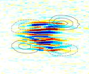
  $Re=520$ are shown in figures 8 and 9. The structures of both the small- and large-scale flows do not change within the range of Reynolds numbers under consideration: elongated streaks dominate as a small-scale feature (see $u^{\prime }$ in figure 8) whereas the large-scale flow has a quadrupolar shape, as illustrated by the black lines of isocontours of the wall-normal vorticity (defined as $\omega _{y*}={\partial u^{\prime \,LSF}_*}/{\partial z_*} - {\partial w^{\prime \,LSF}_*}/{\partial x_*}$) in figures 8 and 9. In addition, in figure 9 we observe that the large-scale flow is composed of both streamwise and spanwise velocity components of similar order of magnitude. The reason why the streamwise velocity component of the large-scale flow is not as pronounced as the spanwise component in the evolution of the measured velocity fluctuations (figure 2) and in premultiplied spectra (figure 5) is simply due to the large amplitude of the small-scale streamwise streaks, which masks the streamwise large-scale flow. Specifically, $u^{\prime }_*$ and $w_*^{\prime }$ are of the order of $10^{-1}$ and $10^{-2}$, respectively.

Figure 8. Sequence of eight pairs of images showing small-scale velocity fluctuation fields for  $Re=520$ and $A=60$. In each pair the top and bottom images correspond to the streamwise ( $u_\ast^\prime$) and spanwise ( $w_\ast^\prime$) velocity fluctuations. The fields are reconstructed by inverse fast Fourier transform for the spectral range $|k_*|>0.86$ ( $|\lambda |<7.3h$). The time instants and the data used in Fourier filtering are the same as presented in figure 2. In addition, solid/dashed black lines represent the isocontours of positive/negative wall-normal vorticity of the large-scale flow reconstructed using the spectral range $|k_*|<0.32$ ( $|\lambda |>19.4h$). The outermost isocontours correspond to $(\omega _y h)/U_{belt}=\pm 0.004$ and each subsequent inward isocontour is increased/decreased by $0.004$.

Figure 9. The same as in figure 8 but for large-scale fluctuations of the velocity and wall-normal vorticity fields. The fields are reconstructed by inverse fast Fourier transform for the spectral range  $|k_*|<0.32$ ( $|\lambda |>19.4h$). The third and sixth rows represent the wall-normal vorticity of the large-scale flow $(\omega _y h)/U_{belt}$. The outermost isocontours correspond to $(\omega _y h)/U_{belt}=\pm 0.004$ and each subsequent inward isocontour is increased/decreased by $0.004$ (same as in figure 8).
Taking advantage of large-scale flow separation at  $\lambda =19.4h$, we determine for the first time the dependence of the large-scale flow intensity on Reynolds number $Re$ and jet amplitude $A$. For this we calculate the mean energy of premultiplied spectra contained within the spectral region $k_* < 0.32$ ( $\lambda >19.4h$). The results are shown in figure 10. The spectral energy distribution shown in figure 5 is not necessarily symmetric around $k_{z*}=0$ – this is the case only if the $u^{\prime }_*$ and $w_*^{\prime }$ fields are perfectly symmetric along the spanwise direction. For this reason, we consider separately two different spectral regions: $k_{z*}>0$ and $k_{z*}<0$. The relative difference between these two regions is small, indicating that the asymmetry in the spanwise direction (or, in other words, the inclination of the large-scale flow) of the localized turbulent spot is weak.

Figure 10. The amplitude of the mean spectral density of premultiplied spectra that corresponds to the large-scale flow ( $|\lambda |>19.4h$) for streamwise (a) and spanwise (b) velocity fluctuations. We present the modes in quadrant I ( $k_{x*}>0,k_{z*}>0$) and in quadrant IV ( $k_{x*}>0,k_{z*}<0$) of premultiplied spectra separately, using squares and plus signs, respectively. Note two different scales on the ordinate axes.
3.3. Initial dynamics of turbulent spot
3.3.1. Coupling between large- and small-scale flows
Here, we consider the initial dynamics of the turbulent spot after the instantaneous jet injection at  $t_*=0$. First, we define the energy of streamwise velocity fluctuations of small-scale flow $u^{\prime \,SSF}_*$ as
 \begin{equation} E_{*}^{SSF}(t_*) = \frac{E^{SSF}(t_*)}{U_{belt}^2} = \frac{\Delta x\,\Delta z}{2S_m} \underset{x}{\overset{}{\sum}}\underset{z}{\overset{}{\sum}} u^{\prime\,SSF}_*(x_*,z_*,t_*)^2 ,\end{equation}
where  $S_m$ is the measurement area. In contrast to the results in Klotz & Wesfreid (Reference Klotz and Wesfreid2017), we normalize the energy with $U_{belt}^2$ and not with the initial energy of the perturbation $E_0$. Next, we define the centroid position of $E_*^{SSF}$ corresponding to the instantaneous position of the barycentre of the streaky structure of the turbulent spot as
 \begin{equation} x_{cen*}(t_*) = \frac{\displaystyle\sum_{x}\sum_{z}(u^{\prime\,SSF}_*(x_*,z_*,t_*))^2x_*} {\displaystyle\sum_{x}\sum_{z}(u^{\prime\,SSF}_*(x_*,z_*,t_*))^2}. \end{equation}
We calculate the instantaneous advection velocity of the spot using the time derivative of  $x_{cen*}(t_*)$:
 \begin{equation} \dot{x}_{cen*}(t_*) = U_{adv*}(t_*) = \frac{\textrm{d}\kern0.7pt x_{cen*}(t_*)}{\textrm{d} t}, \end{equation}
which can be considered as the group velocity of the perturbation field. Finally, we also determine the time evolution of the intensity of the large-scale flow around the turbulent spot by calculating the instantaneous maximal positive value of the large-scale streamwise velocity fluctuations (shown in figure 9):
 \begin{equation} U_{LSF*}=\max\nolimits_{S_m}(u_*^{\prime\,LSF}). \end{equation}
 In figure 11 we plot the time evolutions of  $E_*^{SSF}$, $x_{cen*}$, $U_{adv*}$ and $\max (U_{LSF*})$ for ( $Re=520, A=60$). Each single experimental realization is represented by one thin curve. The red thick solid curves correspond to the time evolution of the quantities averaged over all realizations, which we will refer to as $\bar {E}_*^{SSF}$, $\bar {x}_{cen*}$, $\bar {U}_{adv*}$ and $\max (\bar {U}_{LSF*})$, respectively. In figures 12–14 we show the dependence of these ensemble-averaged quantities on $Re$ and $A$. Note that in figures 13 and 14 the scale on the ordinate corresponds only to the lowest jet amplitude (blue curves). Each subsequent amplitude is shifted upwards by 0.3/0.04 units in figure 13/14 to increase readability. The zero level for each case is presented by the dotted line in the corresponding colour.

Figure 11. Time evolution of: (a) the energy of small-scale flow  $E_*^{SSF}$ normalized with $U_{belt}^2$; (b) the centroid $x_{cen*}$ of the small-scale flow; (c) the advection speed $U_{adv*}$ defined as the time derivative of the centroid $x_{cen*}$ of the small-scale flow; and (d) the maximum of the streamwise component of the large-scale flow $\max (U_{LSF*})$. Each realization is shown by a thin curve and the thick red curves represent the evolution averaged over all realizations. The data shown correspond to $Re=520$ and $A=60$. The vertical dashed magenta line represents the seed time.

Figure 12. Evolution of  $\bar {E}_*^{SSF}$ for different amplitudes and for $Re=380$ (a), $Re=480$ (b) and $Re=520$ (c). The thick lines indicate the time interval for which $0.75\max _t(\bar {E}_*^{SSF})<\bar {E}_*^{SSF}(t_*)<\max _t(\bar {E}_*^{SSF})$.

Figure 13. Evolution of  $\bar {U}_{adv*}$ for different perturbation amplitudes and for $Re=380$ (a), $Re=480$ (b) and $Re=520$ (c). The scale presented on the ordinate corresponds to the lowest amplitude (blue curves). Each subsequent amplitude is shifted upwards by 0.3 units with respect to the previous one in order to increase readability. The zero for each amplitude is marked by the dotted line in the corresponding colour. The thick lines indicate the same time interval as in figure 12.

Figure 14. Evolution of  $\max (\bar {U}_{LSF*})$ for different perturbation amplitudes and for $Re=380$ (a), $Re=480$ (b) and $Re=520$ (c). Each subsequent amplitude is shifted upwards by 0.04 units with respect to the previous one. The zero for each amplitude is marked by the dotted line in the corresponding colour. The thick lines indicate the same time interval as in figure 12.
In order to achieve the highest possible signal-to-noise ratio, we analyse the evolution of the turbulent spot at the time when its structure is the most prominent, i.e. close to the global energy peak  $\max _t(\bar {E}_*^{SSF}(t_*))$ in figure 12. For each combination of $Re$ and $A$, we select the time interval such that $0.75\max _t(\bar {E}_*^{SSF})<\bar {E}_*^{SSF}(t_*)<\max _t(\bar {E}_*^{SSF})$ (indicated by the thick lines in figures 12–14). Finally, for each ( $Re$,
$Re$,  $A$) pair we calculate the time-averaged $\bar {E}_*^{SSF}$, $\bar {U}_{adv*}$ and $\max (\bar {U}_{LSF*})$ within the indicated time intervals. We checked that the effect of the advection of the small-scale flow through the rightmost end of the measurement area does not influence the quantities under consideration in the selected time interval.
Figure 12 illustrates that the energy of small scales increases monotonically with both  $Re$ and $A$. Interestingly, in figure 13 the advection velocity is negative during the first ${\sim }20$ advection units. This is due to the fact that the analysed structures grow transiently from zero, and during this initial period the signature of the localized turbulent spot can be masked by the small variations of the base flow. We call this initial delay needed for the external perturbation to settle (and to form the turbulent spot) as the ‘seed time’; we mark it by the magenta dashed vertical line in figures 11, 13 and 14. Finally, by comparing figure 12 with figure 14, we note that, for most combinations of $Re$ and $A$, the maximum of $\bar {E}_*^{SSF}$ slightly precedes the maximum of $\bar {U}_{LSF*}$.
The dependence of the large-scale flow amplitude ( $\max (\bar {U}_{LSF*})$) on the energy of the small-scale flow ( $\bar {E}_*^{SSF}$) is plotted in figure 15. Different colours mark different Reynolds numbers (blue, red and green correspond to $Re=380$, $Re=480$ and $Re=520$, respectively) and different symbols mark different jet amplitudes (the sequence of diamond, square, triangle, cross and star symbols are in the ascending order of $\langle V_{jet} \rangle _t$). The large-scale flow intensity and the energy of the small-scale flow collapse onto the straight black dashed line for all realizations.

Figure 15. Dependence of the intensity of large-scale flow ( $\max (\bar {U}_{LSF*})$) on the small-scale flow energy ( $\bar {E}_*^{SSF})$. Blue, red and green colours correspond to $Re=380$, $Re=480$ and $Re=520$, respectively. Different symbols represent different amplitude ranges specified in the legend.
Finally, in figure 16, we show that the advection speed of the turbulent spot ( $\bar {U}_{adv*}$) depends nearly linearly on the large-scale flow intensity ( $\max (\bar {U}_{LSF*})$). The colours and symbols are the same as in figure 15. As shown in figure 9 at the right front (upstream with respect to Poiseuille component of the base flow, see Klotz et al. (Reference Klotz, Lemoult, Frontczak, Tuckerman and Wesfreid2017)), the streamwise component of the large-scale flow has a negative value, whereas the opposite is true at the left (downstream) front. However, the positive amplitude on the left of the spot is more important when compared to the negative counterpart on the right. This asymmetry of the large-scale flow contributes to the advection of the turbulent spot to the right.

Figure 16. Dependence of the advection speed of the turbulent spot ( $\bar {U}_{adv*}$) on the large-scale flow intensity ( $\max (\bar {U}_{LSF*})$). Colours and symbols are the same as in figure 15.
3.3.2. Small-scale flow dynamics
In figure 17 we plot the instantaneous velocity fields measured at  $t_*=112$ for $Re=520$ and $A=60$. The first and second rows correspond to the streamwise and spanwise velocity fluctuations. The first and second columns illustrate the total velocity fluctuations ( $u^{\prime }_*,w^{\prime }_*$) and small-scale velocity fluctuations ( $u^{\prime }_{SSF*},w^{\prime }_{SSF*}$), respectively. We estimated the size of the turbulent spot using the complex demodulation of the streamwise component of the small-scale flow (see Klotz et al. (Reference Klotz, Lemoult, Frontczak, Tuckerman and Wesfreid2017) for the description of the method), for which the surrounding laminar background value is used as the threshold. This region is marked by black and magenta contours. One can observe that the small-scale flow is restricted to the area of the turbulent spot (figure 17b,e), whereas the extent of the large-scale flow is larger and spans into the laminar region (figure 17a,c).

Figure 17. Illustration of the spatial distribution of the small-scale flow and dominant wavelengths  $|\lambda|\in (2.1h,5.1h)$ at $t_*=112$ and for $Re=520$ and $A=60$. The first and second rows correspond to the streamwise and spanwise velocity fluctuations, respectively. The first, second and third columns represent PIV measurements, the spatial distribution of the small-scale flow and the envelope of the scales contained within the spectral range $|\lambda| \in (2.1h, 5.2h)$. The envelope shown is calculated as time-averaged over $t_*\in (107,117)$. Note that the envelope colour map (c,f) is represented with logarithmic scale. Black and magenta contours indicate the size of the spot, estimated as the region where the envelope of the streamwise component of the small-scale flow exceeds the value of the surrounding laminar flow. Black contours in panels (b) and (e) mark the regions of $w^{\prime }_{SSF*}=0.012$. The evolution of the energy of the spanwise velocity component of the small-scale flow is shown in the final panel (g).
In addition, by comparing the first and second columns of figure 17, one can observe that the streamwise velocity component  $u^{\prime }_*$ is dominated by small-scale flow (streaks), whereas the spanwise velocity component is dominated by large-scale flow, stretching the turbulent spot in the vertical direction. This is consistent with the results shown in figures2 and 5–7. In addition, the black curves in figure 17(b,e) mark the isocontours of $w^{\prime }_{SSF*}=0.012$, which indicates the spatial distribution of the increased intensity of the spanwise component of the small-scale flow. In figure 17(b) one can observe that the local maxima of the $u^{\prime }_{SSF*}$ (streaks) are not spatially correlated with the local maxima of the $w^{\prime }_{SSF*}$ (rolls), which suggests a spanwise phase shift between the two velocity components of small-scale flow.
In addition, to better illustrate the spatial distribution of the small scales, which corresponds to the broad-band peak  $|\lambda| = 3.1h$ shown in figure 6, we calculate the envelope of the streamwise and spanwise velocity fluctuations contained within the spectral range $|\lambda| \in (2.1h,5.1h)$. The envelope was again calculated using complex demodulation technique and time-averaged over $t_*\in (107,117)$. The results are shown in figure 17(c,f). Owing to the large difference in amplitudes of $u^{\prime }_{SSF*}$ and $w^{\prime }_{SSF*}$, we use the logarithmic scale of the colour map. One can observe that the amplitude of the streaks reaches a maximal value around $x_* \approx 16$ (close to the centre of the turbulent spot), whereas the weak amplitude of $w^{\prime }_{SSF*}$ tends to be concentrated close to the tips of the turbulent spot. Finally, in figure 17(g) we show the evolution of the spanwise velocity component of the small-scale flow $E_{SSF\,w^{\prime }_*}$. Its peak is approximately one order of magnitude lower when compared to the peak of the total velocity fluctuations $E_{w^{\prime }_*}$ (figure 3), which again indicates that the spanwise velocity fluctuations are dominated by the large-scale flow. However, these two peaks occur at a similar instant, and prior to the peak of the streamwise velocity component dominated by the streaks. This time delay between the spanwise and streamwise velocity components can be explained by the dominating role of the lift-up during the initial dynamics of the turbulent spot. The initial perturbation generates a patch of turbulence that consists of rolls. These rolls in turn amplify the streaks and decay faster than the streamwise velocity fluctuations. This problem has been discussed in Waleffe (Reference Waleffe1997) and Liu et al. (Reference Liu, Semin, Klotz, Godoy-Diana, Wesfreid and Mullin2021).
4. Self-sustained turbulent spots and oblique turbulent band
Finally, we present the velocity fluctuations for  $Re=570$ (figures 18 and 19) and $Re=610$ (figure 20) in order to qualitatively illustrate how the structure of the turbulent spot and the shape of the large-scale flow change with increasing Reynolds number. The measurements shown in this section correspond to higher transitional Reynolds numbers, at which the flow becomes intermittent. These results were acquired further downstream from the jet perturbation in the region $x_*\in (55,145)$ and for some time later after the jet injection ( $t_* > 710$ for $Re=570$ and $t_* = 864$ for $Re=610$). The first and second columns of figures 18–20 show the fluctuations of the streamwise $u^{\prime}_*$ and spanwise $w^{\prime}_*$ velocity component. The first row illustrates the velocity fields measured in the plane $y_*=0.33$. The second and third rows correspond to the small- and large-scale flows calculated by filtering instantaneous spatial two-dimensional FFT spectra, in the same way as infigures 8and9. In addition, in the second and third rows we superpose the vector fields of the large-scale flow to better illustrate its direction, similar to Barkley & Tuckerman (Reference Barkley and Tuckerman2007), Fukudome & Iida (Reference Fukudome and Iida2012) and Duguet & Schlatter (Reference Duguet and Schlatter2013).

Figure 18. Illustration of a single realization of a self-sustained spot measured for  $Re=570$ and $A=50$. The first and second columns represent the streamwise $u^\prime_*$ and spanwise $w^\prime_*$ velocity fluctuations, respectively. The first, second and third rows correspond to the PIV measurements, and small-scale and large-scale flow, from top to bottom. Vector fields imposed on (c–f) represent the large-scale flow and correspond to the fields shown in (e,f).

Figure 19. Further examples of a self-sustained spot measured for  $Re=570$ and $A=50$. The measurements were done during different realizations than shown in figure 18. The first and second columns correspond to the streamwise $u^\prime_*$ and spanwise $w^\prime_*$ velocity fluctuations, respectively.

Figure 20. Illustration of an oblique turbulent band measured for  $Re=610$ and $A=47$. For the description of each panel, see figure 18.
The structure of the large-scale flow for a self-sustained spot in figure 18(e,f) is similar to  $Re=520$ shown in figure 9. In contrast to lower Reynolds numbers considered before, the spanwise component of small-scale flow is now more pronounced (compare with figures 8 and 5 in Klotz & Wesfreid (Reference Klotz and Wesfreid2017)). The evolution of turbulent spots at the later stage is not deterministic and their size can change between different realizations, as shown in figures 18(a,b) and 19, in agreement with the energy evolution after reaching the energy peak shown in figure 3.
When the Reynolds number is further increased to  $Re=610$, the structure of the flow response to the perturbation can change from a doubly localized turbulent spot to a single oblique band, as shown in figure 20. If this happens, the shape of the large-scale flow modifies from quadrupolar to oblique. This is presented in figure 20(e,f), which is the first experimental evidence of such an oblique large-scale flow. Its orientation is parallel to the turbulent band and reaches the highest intensity close to the laminar–turbulent interface. In addition, at the ends of the stripe structure, we observe a large circulatory motion similar to that in Fukudome & Iida (Reference Fukudome and Iida2012). The inclination angle of the turbulent band (defined as the separatrix between the positive and negative amplitudes of the velocity component of the large-scale flow) is comparable for both the streamwise (figure 20e) and spanwise (figure 20f) velocity fields. In this case the large-scale flow close to the laminar–turbulent interface sets along the orientation of the turbulent structures, as indicated by Seki & Matsubara (Reference Seki and Matsubara2012).
5. Discussion
In § 3, we present detailed experimental analysis of the large- and small-scale flow dynamics. First, we demonstrate that the scale separation of the velocity field holds in this shear flow. We determine two local minima of spectra at  $\lambda =7.3h$ and $\lambda =19.4h$ (or equivalently $k_{z*}=0.86$ and $k_{z*}=0.32$). In plane Poiseuille flow, Lemoult et al. (Reference Lemoult, Aider and Wesfreid2013) used $\lambda =5h$ as the cutoff value to separate the large and small scales. In plane Couette flow, Duguet & Schlatter (Reference Duguet and Schlatter2013) proposed that the cutoff value can be placed anywhere between $\lambda = 20h$ and $\lambda = 50h$. These spectral ranges are in good agreement with the values obtained here. We also note that in pipe flow (i.e. in a system with one extended dimension), Shih, Hsieh & Goldenfeld (Reference Shih, Hsieh and Goldenfeld2016) used $\lambda =6.28R$ in the streamwise direction (where $R$ is the pipe radius) to extract small-scale dynamics of the turbulence.
Using the scale separation argument, for the first time we extract and characterize the large- and small-scale flow structures created by a turbulent spot in plane Couette–Poiseuille flow. Elongated streaks are the dominating small-scale feature and the large-scale flow has a quadrupolar shape. A similar topology of the large-scale flow has already been observed for different shear flows, both experimentally – by Lemoult et al. (Reference Lemoult, Aider and Wesfreid2013, Reference Lemoult, Gumowski, Aider and Wesfreid2014) in plane Poiseuille flow and also by Couliou & Monchaux (Reference Couliou and Monchaux2015) in plane Couette flow – as well as numerically – by Schumacher & Eckhardt (Reference Schumacher and Eckhardt2001) in flow with stress-free boundaries and streamwise forcing sinusoidal in the wall-normal direction, by Lagha & Manneville (Reference Lagha and Manneville2007), Duguet & Schlatter (Reference Duguet and Schlatter2013), Couliou & Monchaux (Reference Couliou and Monchaux2018) and Kashyap, Duguet & Chantry (Reference Kashyap, Duguet and Chantry2020) in plane Couette flow, and by Kashyap et al. (Reference Kashyap, Duguet and Chantry2020) in Couette–Poiseuille and Poiseuille flows. Breuer & Haritonidis (Reference Breuer and Haritonidis1990) and Breuer & Landahl (Reference Breuer and Landahl1990) observed a similar type of structuring even for a boundary layer, which is spatially evolving shear flow without wall-normal confinement. However, they did not investigate the large-scale flow in detail.
We note that single-point hot-wire measurements of the turbulent spots have already been reported for plane Poiseuille flow (e.g. Klingmann & Alfredsson Reference Klingmann and Alfredsson1991; Klingmann Reference Klingmann1992) and for boundary layer flow (e.g. Amini & Lespinard Reference Amini and Lespinard1982; Bakchinov et al. Reference Bakchinov, Westin, Kozlov and Alfredsson1998; Westin et al. Reference Westin, Bakchinov, Kozlov and Alfredsson1998). However, single-point measurements do not allow one to study instantaneously the temporal evolution and spatial structuring of a turbulent spot. More importantly, in these papers, the large-scale flow was not extracted nor characterized in detail. In a more recent experiment, Seki & Matsubara (Reference Seki and Matsubara2012) measured with the same technique the streamwise velocity component across the laminar–turbulent interfaces in plane Poiseuille flow. In their experiment the turbulence was generated by permanent obstacles at the entrance of the channel, which is different from the instantaneous jet perturbation used in Klotz & Wesfreid (Reference Klotz and Wesfreid2017) and in this work. For this reason, we can only qualitatively compare their measurements of the streamwise velocity component with our results. They observed that the time-averaged streamwise velocity in the bulk flow acts towards the turbulent–laminar interface from both leading and trailing sides. This observation is similar to the spatial distribution of the large-scale flow shown here in figures 9, 18(e) and 20(e), in which both the turbulent spot and oblique turbulent band are compressed in the streamwise direction by the large-scale flow.
Well-controlled instantaneous point-like perturbation, combined with two-dimensional PIV measurements of the in-plane velocity components, gives us the opportunity to study both temporal evolution and spatial structuring of the localized turbulent spot. Taking advantage of the significantly reduced advection speed of the turbulent structures in our experimental set-up, we study in detail the initial dynamics of the turbulent spot. For this we use the energy of the small-scale flow ( $\bar {E}_*^{SSF}$), the advection velocity of the turbulent spot ( $\bar {U}_{adv*}$) and the amplitude of the large-scale flow intensity ( $\max (\bar {U}_{LSF*})$) as the main parameters. First, our results indicate that some finite time is required for the external perturbation to unpack in order to create the turbulent spot. This initial delay (the seed time) is equal to approximately 20 advective time units for the range of parameters studied here. Then, we observe that the energy of the small-scale flow increases monotonically with both $Re$ and $A$. Growth with $Re$ is expected based on the transient growth theory (Schmid & Henningson Reference Schmid and Henningson2001). Increase with perturbation amplitude $A$ can be explained by the localized nature of the perturbation: the larger the amplitude perturbation, the more pronounced is the spatial proliferation of the spot into the laminar region, which results in increase of streak area and leads to the growth of $\bar {E}_*^{SSF}$. In addition, Cherubini et al. (Reference Cherubini, De Palma, Robinet and Bottaro2011) numerically observed a similar increase of the energy of the flow response to the perturbation with energy of the amplitude perturbation.
We demonstrate that the large- and small-scale flow intensities are coupled for the range of parameters under investigation. As illustrated in figure 8 and in the supplementary movie (available at https://doi.org/10.1017/jfm.2020.1089), each vortex of the large-scale quadrupole is centred close to the interface of the laminar flow and turbulent spot, at the location where the streaks have an oblique orientation and lose their continuity along the streamwise direction. As already discussed in the introduction, the large-scale flow (or drift flow) in Rayleigh–Bénard convection is generated by the distortion of the pattern (either through pattern curvature or by the presence of dislocations within the pattern). Our observations suggest that a similar mechanism (deformation and inhomogeneity of the streak pattern) can be associated with the large-scale flow generation in the shear flow. We also show that the advection of the turbulent spot depends on the large-scale flow intensity. This can be explained by the advection of the small scales (streaks) by the large-scale flow. At both upstream and downstream sides of the turbulent spot, the streamwise component of the large-scale flow points towards the centre of the turbulent spot. However, the spatial distribution of this component is asymmetrical in the streamwise direction (i.e. a higher value of the intensity downstream with respect to the Poiseuille component of the base flow and a lower absolute value of the intensity upstream). This streamwise asymmetry induces the drift flow that advects the turbulent spot.
Regarding the initial dynamics of a turbulent spot, our observations can be summarized as follows. The external perturbation after the seed time unpacks and as a result the turbulent spot is formed. During this process the small-scale streaks are amplified through the lift-up mechanism (or equivalently by transient growth). The energy of the small-scale flow and the size of the turbulent spot depend not only on the Reynolds number but also on the amplitude of the perturbation due to spatial localization of the turbulent spot. The irregularity and obliqueness of the streak pattern induces the large-scale flow, the spatial distribution of which is asymmetrical in the streamwise direction. This asymmetry in turns affects the advection velocity of the turbulent spot.
Finally, at higher Reynolds numbers the decay of the turbulent spot becomes postponed due to the non-trivial dynamics of the small-scale flow. This manifests by the increase of the amplitude of the spanwise velocity component of the small-scale flow, which is a signature of the streak destabilization similar to that in Waleffe (Reference Waleffe1997), Duriez et al. (Reference Duriez, Aider and Wesfreid2009) and Dessup et al. (Reference Dessup, Tuckerman, Wesfreid, Barkley and Willis2018). After further increase of the Reynolds number, a doubly localized turbulent spot can change into a single oblique turbulent band. This process is also accompanied by the change of the shape of the large-scale flow from quadrupolar to oblique, with the direction of the flow oriented along the turbulent band. Our direct, precise and spatial measurements of the large-scale flow are in good agreement with existing numerical observations (Barkley & Tuckerman Reference Barkley and Tuckerman2007; Fukudome & Iida Reference Fukudome and Iida2012; Duguet & Schlatter Reference Duguet and Schlatter2013) and confirm the interpretation proposed by Seki & Matsubara (Reference Seki and Matsubara2012) intheir figure 21(b). This is also in contrast to what Coles & Van Atta (Reference Coles and Van Atta1966) suggested in their early experiments of spirals in Taylor–Couette configuration.
6. Conclusions
We present detailed experimental analysis of the localized turbulent structures triggered by a strong impulsive perturbation in the transitional range of Reynolds numbers in plane Couette–Poiseuille flow. In contrast to Klotz & Wesfreid (Reference Klotz and Wesfreid2017), here we consider a wider range of jet amplitudes and analyse in detail the large-scale flow induced around localized turbulent structures. We demonstrate for the first time that the scale separation of velocity field holds in plane Couette–Poiseuille flow and, using this, we extract the large-scale flow from our measurements. The greatly reduced advection velocity of the turbulent structures in our experimental set-up enables us to measure accurately both the spatial structuring and temporal evolution of the weak large-scale flow, and to quantify experimentally the dependence of the large-scale flow intensity on the Reynolds number  $Re$ and forcing amplitude $A$ for a localized turbulent spot. We show that the energy of small scales grows with Reynolds number and with the amplitude of the perturbation. In addition, we show that the small and large scales are coupled for the range of parameters studied here. Moreover, we demonstrate that the advection speed of the turbulent spot depends on the large-scale flow intensity, which can be explained by the asymmetry of the streamwise component of the large-scale flow. Finally, we extend our analysis for higher Reynolds numbers, showing the measurements of the self-sustained localized turbulent spot with postponed decay, and first experimental measurements of the large flow generated around a single oblique turbulent band – in agreement with the numerical results of Barkley & Tuckerman (Reference Barkley and Tuckerman2007), Fukudome & Iida (Reference Fukudome and Iida2012) and Duguet & Schlatter (Reference Duguet and Schlatter2013) and with the interpretation proposed by Seki & Matsubara Reference Seki and Matsubara2012.
Supplementary movie
A supplementary movie is available at https://doi.org/10.1017/jfm.2020.1089.
Acknowledgements
We thank Y. Duguet, S. Gomé, G. Lemoult, T. Liu, B. Semin and L.S. Tuckerman for fruitful discussions.
Funding
This work was supported by a grant, TRANSFLOW, provided by the Agence Nationale de la Recherche (ANR). A.M.P. was partially supported by the French Embassy in Russia (I.I. Mechnikov scholarship) and by the Russian Science Foundation (project no. 18-79-00189). L.K. was partially supported by the European Union's Horizon 2020 research and innovation programme under the Marie Skłodowska-Curie grant agreement no. 754411.
Declaration of interests
The authors report no conflict of interest.
Appendix. Structure of the flow induced by the jet perturbation without shear flow ( $Re=0$)

In order to confirm that the observed quadrupole shape of the large-scale flow is related to the intrinsic properties of the spot in the shear flow and not to the water jet injection used as the forcing, we additionally measure the velocity fields generated by the water jet when the plastic belt is at rest ( $Re=0$, i.e. without the shear flow) and compare these fields to the flow structures triggered by the jet perturbation in the presence of the shear flow for $Re=520$ and $A=60$. In this appendix the jet speed $\langle V_{jet} \rangle _t\simeq 5.63\ \textrm {m}\ \textrm {s}^{-1}$ is used to define the advective time unit and to normalize the measured velocity, since $U_{belt}=0$ for $Re=0$. In figure 21 we present the instantaneous wall-normal vorticity field $\omega _y$ measured at $t_{**}=t\,V_{jet}/h = 4.2 \times 10^{3}$ for $Re=0$ (first column) and $Re=520$ (second column), respectively. This selected instant is also equivalent to $t_{*}=t\,U_{belt}/h=71$ for the case $Re=520$. In figure 21(a) the wall-normal vorticity $\omega _y$ is directly computed from the measured velocity fields $u$ and $w$, whereas the field highlighted in figure 21(c) is obtained from velocity fluctuations $u^{\prime }$ and $w^{\prime }$ after having subtracted the base flow. Finally, in the bottom row (figure 21b,d) we present the wall-normal vorticity of the large-scale flow calculated from the corresponding fields shown in the top row (figure 21a,c) by filtering with a fourth-order Butterworth low-pass filter ( $|\lambda |>19.4h$). The quadrupole is observed only in the presence of the shear flow, even if the amplitude of the water jet is the same for both cases. Note that the colour bar scales in the first and second columns are different. To facilitate the comparison, we mark the maximal values from the first column by black horizontal lines on the colour bar in the second column.

Figure 21. Comparison of the flow structure induced by the jet perturbation at the highest considered amplitude ( $\langle V_{jet} \rangle _t = 5.63\ \textrm {m}\ \textrm {s}^{-1}$) without and with the shear flow (first column for $Re=0$ and second column for $Re=520$, respectively). Vorticity fields are normalized with $\langle V_{jet} \rangle _t$. The upper row represents the instantaneous vorticity field at $t\,V_{jet}/h = 4.2 \times 10^{3}$. The lower row shows the corresponding large-scale flow obtained by spectral filtering with a low-pass Butterworth filter ( $|\lambda |>7.3h$). Note the different scales in the colour bars. To facilitate the comparison, we mark the maximal values from the first column by black horizontal lines on the colour bar in the second column.
Using the same procedure as described in § 3.1, we compute for  $Re=0$ the premultiplied spectra $\langle S_u\rangle _t$ and $\langle S_w\rangle _t$, which are then averaged over 10 realizations and in time ( $0 < t\,V_{jet}/h < 4.2 \times 10^{3}$). The results are shown in figure 22. In figure 23 we compare azimuthally averaged premultiplied spectra $P^{\theta }$ for $Re=0$ (green solid curve) and for $Re=520$ (red solid curve). The prominent peak at small scales for $Re=520$ is absent in the case without the shear flow. Moreover, the amplitude of the large scales averaged over the region marked by the shaded region on the left of figure 23(a,b) ( $|\lambda | \in (32.0h,60.0h)$) is more than two orders of magnitude larger when compared to the case with the belt at rest. The green dotted curves in figure 23(a,b) highlight the standard deviation computed over 10 different realizations for $Re=0$. We consider the standard deviation in two different spectral regions that are marked by shaded areas: $|\lambda | \in (2.4h,4.0h)$ corresponding to the small scales and $|\lambda | \in (32.0h,60.0h)$ that represents the large scales. The standard deviation of the large and small scales is less than $0.2\,\%$ and $1.4\,\%$, respectively, when compared to the premultiplied amplitudes in the analogous spectral ranges for the $Re=520$ case. The variability of the jet perturbation just after the jet injection ( $t_{**} \approx 100$ or $t_{*} \approx 1.7$) is less than $0.5\,\%$. We also approximate the upper bound for the size of the initial perturbation, which is lower than $6h$ in both streamwise and spanwise directions.

Figure 22. The same as in figure 5 but for the case without the shear flow ( $Re=0$) and for the highest amplitude $\langle V_{jet} \rangle _t = 5.63\ \textrm {m}\ \textrm {s}^{-1}$. Premultiplied spectra are normalized with $\langle V_{jet}\rangle _t$ in this case. For reference, we plot the spectral local minima determined for $Re \neq 0$ as magenta dashed ( $\lambda =7.3h$) and blue dashed-dotted ( $\lambda =19.4h$) arcs, respectively. The vertical green line represents the $k_{z*}=0$ axis.

Figure 23. Azimuthally averaged profiles for streamwise  $P^{\theta }_{u^{\prime }}$ (a) and spanwise $P^{\theta }_{w^{\prime }}$ (b) velocity fluctuations. The green solid curve corresponds to $Re=0$. Also the standard deviation is shown by the green dotted curves. For comparison, we also present the profiles for $Re=520$ and $A=60$. All spectra presented here are normalized with $\langle V_{jet} \rangle _t = 5.63\ \textrm {m}\ \textrm {s}^{-1}$. We plot the spectral local minima as the magenta dashed ( $\lambda =7.3h$) and blue dashed-dotted ( $\lambda =19.4h$) lines, respectively. The two spectral ranges marked by the grey shaded regions correspond to $|\lambda | \in (2.4h,4.0h)$ and $|\lambda | \in (32.0h,60.0h)$.
All the above confirms that the perturbation is well controlled, repeatable, small and weak (when compared to the energy of the structures induced in the presence of the shear flow), and that the quadrupole topology is not induced by the jet perturbation.


 Open access