


1. Introduction
Systems of large-scale vortices such as a vortex pair and an array of vortices are often observed in the atmosphere of the Earth and other planets, such as Jupiter and Saturn, and in the oceans (Thorpe Reference Thorpe2005). For example, an array of counter-rotating vortices resembling a von Kármán vortex street is often observed in the wake of an isolated island (Etling Reference Etling1989; Potylitsin & Peltier Reference Potylitsin and Peltier1998). On Jupiter, anticyclones and cyclones formed a von Kármán vortex street for about 50 years (Youssef & Marcus Reference Youssef and Marcus2003). These arrays of vortices can be generated by instabilities of a jet flow and a shear flow (the Kelvin–Helmholtz instability), the baroclinic instability and other mechanisms. The instability of an array of vortices, which is sometimes regarded as a secondary instability, is one of the most fundamental properties that are indispensable for understanding its dynamics and fate. The effect of rotation and stratification on the instability is of great interest because, for example, it can lead to preference in the sense of rotation of the vortices; in fact, the von Kármán vortex street in the wake of an isolated island sometimes becomes asymmetric, with anticyclonic vortices being nearly destroyed (Potylitsin & Peltier Reference Potylitsin and Peltier1998; Stegner, Pichon & Beunier Reference Stegner, Pichon and Beunier2005).
There exist several types of instability in the vortices in rotating stratified fluids: the elliptic instability (Miyazaki & Fukumoto Reference Miyazaki and Fukumoto1992; Miyazaki Reference Miyazaki1993; Leblanc & Cambon Reference Leblanc and Cambon1998; Leweke & Williamson Reference Leweke and Williamson1998; Miyazaki & Adachi Reference Miyazaki and Adachi1998; Leblanc Reference Leblanc2000; Otheguy, Billant & Chomaz Reference Otheguy, Billant and Chomaz2006a; Le Dizès Reference Le Dizès2008; Aspden & Vanneste Reference Aspden and Vanneste2009; Guimbard et al. Reference Guimbard, Le Dizès, Le Bars, Le Gal and Leblanc2010), the centrifugal instability (Rayleigh Reference Rayleigh1917; Kloosterziel & van Heijst Reference Kloosterziel and van Heijst1991; Leblanc & Cambon Reference Leblanc and Cambon1998; Potylitsin & Peltier Reference Potylitsin and Peltier1998, Reference Potylitsin and Peltier1999), the zigzag instability (Billant Reference Billant2000; Billant & Chomaz Reference Billant and Chomaz2000a,Reference Billant and Chomazb,Reference Billant and Chomazc; Otheguy, Billant & Chomaz Reference Otheguy, Billant and Chomaz2006b; Deloncle, Billant & Chomaz Reference Deloncle, Billant and Chomaz2008; Waite & Smolarkiewicz Reference Waite and Smolarkiewicz2008; Billant et al. Reference Billant, Deloncle, Chomaz and Otheguy2010) and the radiative instability (Le Dizès & Billant Reference Le Dizès and Billant2009), while the transient growth (Arratia, Caulfield & Chomaz Reference Arratia, Caulfield and Chomaz2013; Gau & Hattori Reference Gau and Hattori2014) is also sometimes important. One of the important characteristics of the arrays of vortices is that there exist hyperbolic points, which add the hyperbolic instability to the above list of instabilities. The hyperbolic instability can be further classified into the pure-hyperbolic instability (Friedlander & Vishik Reference Friedlander and Vishik1991; Lifschitz & Hameiri Reference Lifschitz and Hameiri1991; Sipp & Jacquin Reference Sipp and Jacquin1998; Pralits, Giannetti & Brandt Reference Pralits, Giannetti and Brandt2013), the strato-hyperbolic instability (Suzuki, Hirota & Hattori Reference Suzuki, Hirota and Hattori2018; Hattori et al. Reference Hattori, Suzuki, Hirota and Khandelwal2021) and the rotational-hyperbolic instability (Sipp, Lauga & Jacquin Reference Sipp, Lauga and Jacquin1999; Godeferd, Cambon & Leblanc Reference Godeferd, Cambon and Leblanc2001; Hattori & Hirota Reference Hattori and Hirota2023).
The stability of arrays of vortices has been investigated by several authors. Leblanc & Cambon (Reference Leblanc and Cambon1998) investigated the linear stability of the Stuart vortices in rotating non-stratified fluids by numerical analysis; the centrifugal, elliptic and pure-hyperbolic instabilities were found. Leblanc & Godeferd (Reference Leblanc and Godeferd1999) showed the structures of a mode of the pure-hyperbolic instability in the two-dimensional (2-D) Taylor–Green vortices by direct numerical simulation. Potylitsin & Peltier (Reference Potylitsin and Peltier1998) investigated the stability of periodic vortices in rotating stratified fluids by numerical analysis; the base flow is a quasi-steady state obtained by relaxation at low Reynolds numbers. According to them, anticyclonic vortices are strongly destabilized by weak rotation, but stabilized by strong rotation; they also claimed that strong stratification stabilizes the vortices. These results were obtained from numerical simulations with limited resolution at low Reynolds numbers. Potylitsin & Peltier (Reference Potylitsin and Peltier1999) investigated the stability of the Stuart vortices in rotating non-stratified fluids by numerical analysis. Three types of instability were found: the elliptic, the centrifugal and the (pure) hyperbolic instabilities.
In our previous work (Hattori et al. Reference Hattori, Suzuki, Hirota and Khandelwal2021), the linear stability of a periodic array of vortices in non-rotating stratified fluids has been investigated in detail; the effects of rotation were studied in Hattori & Hirota (Reference Hattori and Hirota2023), while the base flow was fixed to the 2-D Taylor–Green vortices. The latter work revealed several important aspects of the stability of a periodic array of vortices in rotating stratified fluids. Five types of instability have been shown to appear in general: the pure-hyperbolic instability, the strato-hyperbolic instability, the rotational-hyperbolic instability, the centrifugal instability and the elliptic instability. The condition for each instability and the estimate of the growth rate were obtained in the framework of local stability analysis and proved useful in predicting which instability is dominant for a given set of parameters. However, our understanding is still incomplete because the above results were limited to a particular base flow. Further studies are needed to explore how the stability properties depend on multiple key parameters: the rotation rate of the system, the strength of stratification and the vorticity distribution, which is partially characterized by the strain rates at the stagnation points and the maximum vorticity.
In this paper, we study the linear stability of the Stuart vortices in rotating stratified fluids. We clarify how the growth rate and other characteristics of the instability depend on rotation, stratification and vorticity distribution. There are important reasons for studying the stability of the Stuart vortices after our detailed stability analysis of the 2-D Taylor–Green vortices (Hattori & Hirota Reference Hattori and Hirota2023). First, the Stuart vortices are often regarded as a model of vortices that develop in a mixing layer as a result of the Kelvin–Helmholtz instability; understanding the stability of the Stuart vortices should be important because mixing layers are observed frequently in the atmosphere and the oceans. Next, it is important to investigate how the opposite-signed vortices, which exist in the 2-D Taylor–Green vortices but do not in the Stuart vortices, affect the stability properties. Finally, the instability condition and the estimate of the growth rate derived for each instability in Hattori & Hirota (Reference Hattori and Hirota2023) has been shown to be effective only for the 2-D Taylor–Green vortices; they should be tested for a different base flow that has different magnitudes of strain rates and vorticity, to show their applicability to general base flows. Although there are several works on the stability of the Stuart vortices with or without rotation (Pierrehumbert & Widnall Reference Pierrehumbert and Widnall1982; Leblanc & Cambon Reference Leblanc and Cambon1998; Potylitsin & Peltier Reference Potylitsin and Peltier1999; Godeferd et al. Reference Godeferd, Cambon and Leblanc2001), there is no work on the effects of stratification on the stability of the Stuart vortices. The stability of Kelvin–Helmholtz billows in stratified fluids was studied by Aravind, Dubos & Mathur (Reference Aravind, Dubos and Mathur2022); in their work, however, the vorticity of the base flow and the gravity force are orthogonal, while they are parallel in the present work. We also show the existence of an unstable mode predicted only by theory (the ‘ring mode’ of the elliptic instability; Le Dizès Reference Le Dizès2008).
This paper is organized as follows. In § 2 the problem is formulated; concise expressions for the instability conditions and the estimates of the growth rates, which have been introduced in Hattori & Hirota (Reference Hattori and Hirota2023) in the framework of local stability analysis, are also summarized briefly. The methods of the numerical stability analysis are explained in § 3. The results of local and modal stability analysis are presented together with their comparison in § 4. We conclude in § 5.
2. Problem formulation
2.1. Governing equations
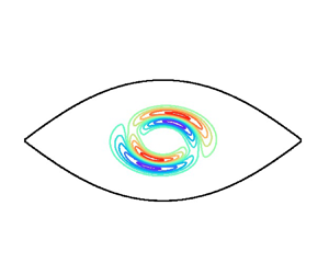
We consider the linear stability of the Stuart vortices in stably stratified and rotating fluids. The Stuart vortices are a one-dimensional array of periodic vortices with vorticity of the same sign (figure 1). The streamfunction and the vorticity are
 $$\begin{gather} \psi = \log{\left(C\cosh{y}+\sqrt{C^2-1}\cos{x}\right)}, \end{gather}$$
 $$\begin{gather}\boldsymbol{\omega}_b = \omega_b(x,y)\,\boldsymbol{e}_z, \quad \omega_b(x,y) ={-}\frac{1}{\left(C\cosh{y}+\sqrt{C^2-1}\cos{x}\right)^2}, \end{gather}$$
where  $C \geqslant 1$ is a constant. In the previous works (Leblanc & Cambon Reference Leblanc and Cambon1998; Godeferd et al. Reference Godeferd, Cambon and Leblanc2001), a different expression, $\psi = \log {(\cosh {y}+\rho _s\cos {x})}$, is used instead of the above streamfunction; the two are related by $\rho _s=\sqrt {1-C^{-2}}$, with a constant that does not affect the flow field. Two adjacent vortices are connected by a hyperbolic point. The vorticity is parallel to the vertical direction, which coincides with the direction of gravity force. The effects of density stratification are taken into account by the Boussinesq approximation. Then the Stuart vortices are steady in the absence of diffusion (Hattori & Hirota Reference Hattori and Hirota2023).

Figure 1. Stuart vortices: (a) streamlines and (b) contours of vorticity distribution for  $C=1.2$; (c) comparison of vorticity distribution on $y=0$ between $C=1.2$ (solid line), $1.6$ (dotted line) and $2$ (dashed line). In (a), the red, green and blue lines show the closed streamlines, the separatrix and the open streamlines, respectively.
Viscosity is taken into account in general, while diffusion of density is neglected since its effects are negligible (Hattori et al. Reference Hattori, Suzuki, Hirota and Khandelwal2021). The base flow is assumed steady because the growth of instabilities is much faster than the time evolution of the base flow due to viscous diffusion in the high-Reynolds-number flows considered in this paper. The velocity, pressure and density fields are decomposed as
 $$\begin{gather} \boldsymbol{u}=\boldsymbol{u}_b+\boldsymbol{u}', \end{gather}$$
 $$\begin{gather}p=p_b+p', \end{gather}$$
 $$\begin{gather}\rho=\rho_{0}+{\alpha}z+\rho', \end{gather}$$
where  $(\boldsymbol {u}_b, p_b, \rho _b=\rho _0 +\alpha z)$ and $(\boldsymbol {u}', p', \rho ')=(u'_x, u'_y, u'_z, p', \rho ')$ are the base flow and the disturbance, the direction of the gravity force is taken as $-\boldsymbol {e}_z$, and the base density is assumed to be $\rho _b=\rho _0+\alpha z$, with $\alpha =\partial \rho _b/\partial z<0$ being a constant. The magnitude of the disturbance is infinitesimally small. Then the governing equations in non-dimensionalized form are
 $$\begin{gather} \boldsymbol{\nabla}\boldsymbol{\cdot}\boldsymbol{u}'=0, \end{gather}$$
 $$\begin{gather}\frac{\partial{\boldsymbol{u}'}}{\partial t}+(\boldsymbol{u}'\boldsymbol{\cdot}\boldsymbol{\nabla})\boldsymbol{u}_b+(\boldsymbol{u}_b\boldsymbol{\cdot}\boldsymbol{\nabla})\boldsymbol{u}' - \frac{1}{Ro}\,\boldsymbol{e}_z \times \boldsymbol{u}' ={-}\boldsymbol{\nabla}{p'}-\rho'\boldsymbol{e}_z+\frac{1}{Re}\,\nabla^2 \boldsymbol{u}', \end{gather}$$
 $$\begin{gather}\frac{\partial{\rho'}}{\partial{t}}+(\boldsymbol{u}_b\boldsymbol{\cdot}\boldsymbol{\nabla}){\rho'}-\frac{1}{F_h^2}\,u'_z =0, \end{gather}$$
where  $Ro =U_0/(2 \varOmega _0 L_0)$ is the Rossby number, $Re =U_0L_0/\nu$ is the Reynolds number, $F_h=U_0/(L_0N)$ is the Froude number based on the horizontal scale, $N=\sqrt {-{\alpha }g/{\rho }_0}$ is the Brunt–Väisälä frequency, $g$ is the acceleration of gravity, $\nu$ is the kinematic viscosity, $\varOmega _0$ is the angular velocity, and $U_0$ and $L_0$ are a characteristic velocity and a length scale, respectively. As in our previous works (Suzuki et al. Reference Suzuki, Hirota and Hattori2018; Hattori et al. Reference Hattori, Suzuki, Hirota and Khandelwal2021), we set $L_0=2{\rm \pi}$, which is the spatial period in the $x$ direction, while $U_0$ is set to the maximum velocity $1$. In the following, the values are scaled by $U_0$ and $L_0$ unless stated explicitly. It is pointed out that the minus sign of the Coriolis force in (2.7) is introduced because the vorticity distribution of the Stuart vortices in (2.2a,b) is negative; $Ro>0$ and $Ro<0$ correspond to the cyclonic and anticyclonic cases, respectively.
In the local stability analysis, the disturbance is assumed to be in the form of a wave packet:
 $$\begin{gather} \boldsymbol{u}'=\left(\hat{\boldsymbol{u}}_0+\delta\hat{\boldsymbol{u}}_1+\cdots \right)\exp \left(\frac{{\rm i}}{\delta}\,\varPhi\right), \end{gather}$$
 $$\begin{gather}p'=\left(\hat{p}_0+\delta\hat{p}_1+\cdots \right)\exp\left(\frac{{\rm i}}{\delta}\,\varPhi\right), \end{gather}$$
 $$\begin{gather}\rho'=\left(\hat{\rho}_0+\delta\hat{\rho}_1+\cdots \right)\exp\left(\frac{{\rm i}}{\delta}\,\varPhi\right), \end{gather}$$
where  $\delta$ is a small parameter, and $\varPhi$ is eikonal, satisfying ${\rm D}\varPhi /{\rm D}t=0$ (where ${\rm D}/{\rm D}t=\partial /\partial t+ \boldsymbol {u}_b \boldsymbol {\cdot } \boldsymbol {\nabla }$). Viscosity is neglected in the local stability analysis. Substituting the above expressions into (2.6)–(2.8) yields a set of ordinary differential equations at the leading order:
 $$\begin{gather} {\frac{{\rm{d}} {{\boldsymbol{X}}}}{{\rm{d}} {t}}} = {\boldsymbol{U}}({\boldsymbol{X}}), \end{gather}$$
 $$\begin{gather}{\frac{{\rm{d}} {{\boldsymbol{k}}}}{{\rm{d}} {t}}} ={-}{\boldsymbol{\mathsf{L}}}^{\rm T} {\boldsymbol{k}}, \end{gather}$$
 $$\begin{gather}{\frac{{\rm{d}} {{\boldsymbol{a}}}}{{\rm{d}} {t}}} = \left( 2{\hat{\boldsymbol{k}}}{\hat{\boldsymbol{k}}}^{\rm T} - {\boldsymbol{\mathsf{I}}} \right) {\boldsymbol{\mathsf{L}}}{\boldsymbol{a}} +\left({\hat{\boldsymbol{k}}}{\hat{\boldsymbol{k}}}^{\rm T}-{\boldsymbol{\mathsf{I}}}\right)r\boldsymbol{e}_z - \frac{1}{Ro} \left( {\hat{\boldsymbol{k}}}{\hat{\boldsymbol{k}}}^{\rm T} - {\boldsymbol{\mathsf{I}}} \right) {\boldsymbol{e}_z} \times {\boldsymbol{a}}, \end{gather}$$
 $$\begin{gather}\frac{{\rm d}r}{{\rm d}t}= \frac{1}{F_h^2}\,a_z, \end{gather}$$
where  ${\boldsymbol{\mathsf{L}}}_{ij} = \partial U_i/\partial x_j$ and $\hat {\boldsymbol {k}}=\boldsymbol {k}/|{\boldsymbol {k}}|$ (Friedlander & Vishik Reference Friedlander and Vishik1991; Lifschitz & Hameiri Reference Lifschitz and Hameiri1991; Leblanc Reference Leblanc1997). Here, ${\boldsymbol {X}}$ is the position of the fluid particle, and $\boldsymbol {k}=\boldsymbol {\nabla }\varPhi$ is the local wavevector, while ${\boldsymbol {a}}=\hat {\boldsymbol {u}}_0$ and $r=\hat {\rho }_0$ are the amplitudes of the disturbance corresponding to velocity and density, respectively. The incompressibility condition (2.6) leads to ${\boldsymbol {a}} \boldsymbol {\cdot } {\boldsymbol {k}} = 0$, which is satisfied for $t>0$ if it holds at $t=0$. The base flow is unstable if the amplitude $\{{\boldsymbol {a}}, r\}$ grows without bound.
The number of variables in (2.14) and (2.15) can be reduced from four to three by introducing
 \begin{equation} p = \frac{k}{k_\perp}\,{\boldsymbol{k}}_\perp \boldsymbol{\cdot}{\boldsymbol{a}}_\perp{=}{-}\frac{kk_z}{k_\perp}\,a_z, \quad q = \left(\frac{k}{k_\perp}\,{\boldsymbol{k}}_\perp{\times} {\boldsymbol{a}}_\perp\right)\boldsymbol{\cdot}{\boldsymbol{e}}_z, \quad s = \frac{k}{k_\perp}\,r \end{equation}
as in Bayly, Holm & Lifschitz (Reference Bayly, Holm and Lifschitz1996), where  $\boldsymbol {k}_\perp =(k_x, k_y)^{\rm T}$, $\boldsymbol {a}_\perp =(a_x, a_y)^{\rm T}$ and
 \begin{equation}
{\boldsymbol{\mathsf{L}}} = \left(\begin{array}{@{}cc@{}}
{\boldsymbol{\mathsf{L}}}_\perp & 0 \\ 0 & 0
\end{array} \right), \quad {\boldsymbol{\mathsf{H}}} =
{\boldsymbol{\mathsf{L}}}_\perp \left(
\begin{array}{@{}cc@{}} 0 & 1 \\ -1 & 0 \end{array} \right).
\end{equation}
\begin{equation}
{\boldsymbol{\mathsf{L}}} = \left(\begin{array}{@{}cc@{}}
{\boldsymbol{\mathsf{L}}}_\perp & 0 \\ 0 & 0
\end{array} \right), \quad {\boldsymbol{\mathsf{H}}} =
{\boldsymbol{\mathsf{L}}}_\perp \left(
\begin{array}{@{}cc@{}} 0 & 1 \\ -1 & 0 \end{array} \right).
\end{equation}
Then the equations (2.14) and (2.15) reduce to
 \begin{equation} \dfrac{{\rm d}}{{\rm
d}t}\left( \begin{array}{@{}c@{}}p\\q\\s\end{array}\right) =
\left(\begin{array}{@{}ccc@{}} \dfrac{{\rm d}}{{\rm
d}t}\log{\dfrac{|\boldsymbol{k}_\perp|}{|\boldsymbol{k}|}}
&
\dfrac{2k^2_z\boldsymbol{\mathsf{H}}\boldsymbol{k}_\perp
\boldsymbol{\cdot}\boldsymbol{k}_\perp}{|\boldsymbol{k}|^2\,|\boldsymbol{k}_\perp|^2}+\dfrac{k_z^2}{Ro\,k^2}
&
\dfrac{|\boldsymbol{k}_\perp|^2}{|\boldsymbol{k}|^2}\,k_z\\
-\omega_z-{Ro^{{-}1}} & -\dfrac{{\rm d}}{{\rm
d}t}\log{\dfrac{|\boldsymbol{k}_\perp|}{|\boldsymbol{k}|}}
& 0\\ -\dfrac{1}{F_h^2 k_z} & 0 & -\dfrac{{\rm
d}}{{\rm
d}t}\log{\dfrac{|\boldsymbol{k}_\perp|}{|\boldsymbol{k}|}}
\end{array}\right)\left( \begin{array}{@{}c@{}}
p\\q\\s\end{array}\right).
\end{equation}
\begin{equation} \dfrac{{\rm d}}{{\rm
d}t}\left( \begin{array}{@{}c@{}}p\\q\\s\end{array}\right) =
\left(\begin{array}{@{}ccc@{}} \dfrac{{\rm d}}{{\rm
d}t}\log{\dfrac{|\boldsymbol{k}_\perp|}{|\boldsymbol{k}|}}
&
\dfrac{2k^2_z\boldsymbol{\mathsf{H}}\boldsymbol{k}_\perp
\boldsymbol{\cdot}\boldsymbol{k}_\perp}{|\boldsymbol{k}|^2\,|\boldsymbol{k}_\perp|^2}+\dfrac{k_z^2}{Ro\,k^2}
&
\dfrac{|\boldsymbol{k}_\perp|^2}{|\boldsymbol{k}|^2}\,k_z\\
-\omega_z-{Ro^{{-}1}} & -\dfrac{{\rm d}}{{\rm
d}t}\log{\dfrac{|\boldsymbol{k}_\perp|}{|\boldsymbol{k}|}}
& 0\\ -\dfrac{1}{F_h^2 k_z} & 0 & -\dfrac{{\rm
d}}{{\rm
d}t}\log{\dfrac{|\boldsymbol{k}_\perp|}{|\boldsymbol{k}|}}
\end{array}\right)\left( \begin{array}{@{}c@{}}
p\\q\\s\end{array}\right).
\end{equation}
2.2. Instability condition and estimate of growth rates
Here, we summarize the condition and the estimate of the growth rate for each instability obtained in the framework of local stability analysis; see Hattori & Hirota (Reference Hattori and Hirota2023) for the details. It is pointed out that our aim here is to give compact and useful expressions for the instability condition and the growth rate for each instability, which are not always rigorous but allow us to interpret the results in § 4 without difficulties. In the following,  $C_{PH}$, $C_{SH}$, $C_{RH}$, $C_{C}$ and $C_{E}$ are $O(1)$ coefficients that depend on the parameters in general; the actual dependence will be checked numerically in § 4.1 (figure 8).
(i) Pure-hyperbolic instability. The pure-hyperbolic (PH) instability is due to stretching near the hyperbolic stagnation points. It occurs when
(2.19)The growth rate is estimated as \begin{equation} |{Ro^{{-}1}}| < \varepsilon_h. \end{equation}(2.20)\begin{equation} \sigma = C_{PH} \left(\varepsilon_h^2 -Ro^{{-}2}\right)^{1/2}. \end{equation}
(ii) Strato-hyperbolic instability. The strato-hyperbolic (SH) instability is a variant of the pure-hyperbolic instability under stratification effects. It occurs when the exponential growth near the hyperbolic stagnation points is connected with phase shift due to the inertia-gravity waves in favour of exponential growth. It occurs when
(2.21a,b)The growth rate is estimated as\begin{equation} |{Ro^{{-}1}}| < \varepsilon_h \quad\mbox{and} \quad {F_h^{{-}1}} \gtrsim \omega_{max}/2. \end{equation}(2.22)\begin{equation} \sigma = C_{SH} \left(\varepsilon_h^2 -Ro^{{-}2}\right)^{1/2}. \end{equation}(iii) Rotational-hyperbolic instability. The rotational-hyperbolic (RH) instability is also a variant of the pure-hyperbolic instability. It occurs when
(2.23)The growth rate is estimated as\begin{equation} |{Ro^{{-}1}}| \gtrsim \varepsilon_h. \end{equation}(2.24)\begin{equation} \sigma = C_{RH} \varepsilon_h. \end{equation}(iv) Centrifugal instability. The essential mechanism of the centrifugal (C) instability was given by Rayleigh (Reference Rayleigh1917). It occurs when positive energy is released by interchanging fluid elements under conservation of angular momentum. Assuming a monotonically decreasing vorticity distribution, the instability condition turns out to be
(2.25)The growth rate is estimated as\begin{equation} {-}\omega_{max} < {Ro^{{-}1}} < 0. \end{equation}(2.26)\begin{equation} \sigma = C_{C} \omega_{{max}}. \end{equation}(v) Elliptic instability. The elliptic (E) instability is caused by resonance due to strain at elliptic stagnation points. It occurs when
(2.27a,b)or\begin{equation} {F_h^{{-}1}}<\tfrac{1}{2}\omega_{max} \quad\mbox{and} \quad {Ro^{{-}1}} <{-}\tfrac{3}{2}\omega_{max} \mbox{or} \ {Ro^{{-}1}} >{-}\tfrac{1}{2}\omega_{max}, \end{equation}(2.28a,b)The growth rate is estimated as\begin{equation} {F_h^{{-}1}}>\tfrac{1}{2}\omega_{max} \quad \mbox{and} \quad {-\tfrac{3}{2}}\omega_{max}<{Ro^{{-}1}} \lesssim 0. \end{equation}(2.29)The coefficient\begin{equation} \sigma = C_{E} \varepsilon_e. \end{equation}$C_{E}$ can be expressed as a function of $F_h$ and $Ro$ at the elliptic stagnation point (Leblanc Reference Leblanc2000).


The values of the strain rates  $\varepsilon _h$ and $\varepsilon _e$ at the hyperbolic and elliptic stagnation points, respectively, and the maximum magnitude of vorticity $\omega _{max}$, which appear in the expressions above, are listed in table 1, which includes those for the 2-D Taylor–Green vortices considered in Hattori & Hirota (Reference Hattori and Hirota2023) for comparison purposes. It is pointed out that $\omega _{max}$ and $\varepsilon _e$ of the Stuart vortices are larger than values for the 2-D Taylor–Green vortices, while $\varepsilon _h$ is not much different between the two base flows.
Table 1. Strain rates at hyperbolic and elliptic stagnation points, and maximum vorticity of the Stuart vortices considered in the present paper. The values for the 2-D Taylor–Green vortices studied in Hattori & Hirota (Reference Hattori and Hirota2023) (HH2023) are also included for comparison.

3. Numerical procedure
3.1. Local stability analysis
The numerical method for local stability analysis is same as that in Hattori & Hirota (Reference Hattori and Hirota2023). Equations (2.12)–(2.15) were integrated by the fourth-order Runge–Kutta method. We consider periodic orbits of fluid particles throughout this paper. We also assume that the wavevector  $\boldsymbol {k}$ is time-periodic, which is a necessary condition for exponential instability on the periodic orbits. It is known that $\boldsymbol {k}$ is time-periodic if it is perpendicular to the streamline initially (Lifschitz & Hameiri Reference Lifschitz and Hameiri1993; Hattori & Fukumoto Reference Hattori and Fukumoto2003):
 \begin{equation} \boldsymbol{k}(0)\boldsymbol{\cdot}\boldsymbol{u}_b(\boldsymbol{X}(0))=0. \end{equation}
Then the time evolution of amplitude is described by a Floquet matrix  $\boldsymbol{\mathsf{F}}$ since the matrices that appear in (2.14) are also time-periodic:
 \begin{equation} \{ \boldsymbol{a}, r\}(t+T)=\boldsymbol{\mathsf{F}}(T)\,\{ \boldsymbol{a}, r\}(t), \end{equation}
where  $T$ is the period of $\boldsymbol {k}$ that coincides with that of the particle motion $\boldsymbol {X}$ (Lifschitz & Hameiri Reference Lifschitz and Hameiri1993; Hattori & Fukumoto Reference Hattori and Fukumoto2003). Our task is to calculate the eigenvalues $\{ \mu _i \}$ of $\boldsymbol{\mathsf{F}}(T)$, which determines the growth rate as
 \begin{equation} \sigma_i=\frac{\log{|\mu_i|}}{T}. \end{equation}
 The initial conditions should be specified to have particular solutions for a given set of the Rossby number  $Ro$ and the Froude number $F_h$. One parameter, which is denoted by $\beta$ in the following subsections, is required for $\boldsymbol {X}(0)$ to identify a streamline in a 2-D flow. We set
 \begin{equation} \boldsymbol{X}(0)=\left({\rm \pi}, \beta y_c, 0\right)^{\rm T},\end{equation}
where  $y_c=\cosh ^{-1}(1+2\sqrt {1-C^{-2}})$ is the maximum of $y$ on the separatrix. The elliptic stagnation point corresponds to $\beta =0$, while $\beta =1$ corresponds to the separatrix. The open streamlines corresponding to $\beta >1$ are also considered.
Another parameter is required for  $\boldsymbol {k}(0)$ to specify the direction of the wavevector that satisfies (3.1); we take the angle between $\boldsymbol {e}_z$ and $\boldsymbol {k}(0)$, which is denoted by $\theta _0$. It should be pointed out that the magnitude of $\boldsymbol {k}(0)$ is arbitrary since the right-hand side of (2.14) depends only on the direction of $\boldsymbol {k}$ and is independent of the magnitude after taking the short-wave limit. For the amplitudes $\boldsymbol {a}(0)$ and $r(0)$, three independent initial conditions satisfying the incompressibility condition $\boldsymbol {a}(0)\boldsymbol {\cdot } \boldsymbol {k}(0)=0$ are considered; the results do not depend on the choice of the initial conditions since the space spanned by the three initial conditions is common. As a result, we obtain the largest growth rate $\sigma$ as a function of $\beta$, $\theta _0$, $Ro$ and $F_h$, namely $\sigma =\sigma (\beta, \theta _0, Ro, F_h)$.
3.2. Modal stability analysis
In the modal stability analysis, (2.6)–(2.8) were solved numerically by the Fourier spectral method (Peyret Reference Peyret2010), assuming periodic boundary conditions in all three directions as in Hattori et al. (Reference Hattori, Suzuki, Hirota and Khandelwal2021) and Hattori & Hirota (Reference Hattori and Hirota2023). Since the Stuart vortices are periodic in  $x$ but not in $y$, the vortices are placed at $y=nL_y$, and those with the opposite-signed vorticity are placed at $y=(n+1/2)L_y$, for $n=0, \pm 1, \pm 2, \ldots\,$, to make the base flow periodic in $y$. The spatial period $L_y$ is fixed at $L_y=4L_0=8{\rm \pi}$, which is large enough to make the effects of the periodic boundary condition in the $y$ direction negligible (Hattori et al. Reference Hattori, Suzuki, Hirota and Khandelwal2021). The time marching was performed by the fourth-order Runge–Kutta method.
Since the base flow is 2-D, the time evolution of disturbances is separable in the vertical direction. Thus we set
 \begin{equation} \boldsymbol{u}' = \exp({{\rm{i}} [\mu (x/L_x) +k_z z]}) \sum_{k_x={-}K_x}^{K_x}\sum_{k_y={-}K_y}^{K_y} \tilde{\boldsymbol{u}}_{k_x,k_y} \exp({{\rm i} [k_x (x/L_x)+k_y (\kern0.7pt y/L_y)]}), \end{equation}
with similar expressions for  $p'$ and $\rho '$. In the above equation, we have included the Floquet exponent ${\rm {i}}\mu$ to consider Floquet modes in general. The number of the Fourier modes is $1024 \times 4096$, as in Hattori et al. (Reference Hattori, Suzuki, Hirota and Khandelwal2021).
The growth rate and frequency were obtained by the method of Krylov subspaces (Edwards et al. Reference Edwards, Tuckerman, Friesner and Sorensen1994; Julien, Ortiz & Chomaz Reference Julien, Ortiz and Chomaz2004; Donnadieu et al. Reference Donnadieu, Ortiz, Chomaz and Billant2009; Hattori et al. Reference Hattori, Suzuki, Hirota and Khandelwal2021; Hattori & Hirota Reference Hattori and Hirota2023). Starting from randomized initial conditions, (2.6)–(2.8) were integrated for a certain long time. Intermediate states  $\{(\boldsymbol {u}'(T_0), \rho '(T_0))$, $(\boldsymbol {u}'(T_0\,{+}\,\Delta T), \rho '(T_0\,{+}\,\Delta T)), \ldots, (\boldsymbol {u}'(T_0+(N_K\,{-}\,1)\,\Delta T), \rho '(T_0+(N_K-1)\,\Delta T))\}$ were used as generators of the Krylov subspace. Then the eigenvalues and the eigenmodes were obtained in the $N_K$-dimensional Krylov subspace. In this method, the error of an eigenvalue $\lambda$ of a linear operator ${\boldsymbol{\mathsf{L}}}$ can be evaluated by
 \begin{equation} \epsilon = \frac{\| {\boldsymbol{\mathsf{L}}}\boldsymbol{v}-\lambda\boldsymbol{v} \|}{\| \boldsymbol{v} \|}, \end{equation}
where  $\boldsymbol {v}$ is the corresponding approximate eigenvector. The error $\epsilon$ depends on the initial time of the data $T_0$, the interval between the data $\Delta T$, and the dimension of the Krylov subspace $N_K$. In order to obtain eigenvalues accurately, several Krylov subspaces were generated from different sets of parameters, and the eigenvalue with the smallest error for each eigenmode was chosen. The actual values of the parameters were chosen after trial and error; $N_K$ was $5$,
$5$,  $10$ or $20$, and $T_0=92, 112, \ldots, 192$, while $\Delta T$ was fixed at $2$. Typically, the error of the eigenvalue is $\epsilon =O(10^{-10})$ for the largest eigenvalue for a fixed wavenumber $k_z$, while it increases for subdominant eigenmodes. In the following, we discarded the eigenmodes with $\epsilon \geqslant 10^{-3}$.
It turned out that the growth rates of the cyclonic case are sometimes difficult to obtain because they are smaller than those of the anticyclonic case. Therefore, we applied a filter that damps the anticyclonic modes and keeps the cyclonic modes unchanged, to obtain the growth rates of the cyclonic case.
3.3. Realizability as a mode
As we will see later, in § 4, the instabilities that are found by local stability analysis are not always found in modal stability analysis at finite Reynolds numbers since high-wavenumber modes are damped by viscous damping. In this case, the corresponding region of the instability in the  $(\beta, \theta _0)$ plane is often thin so that it is difficult to construct an unstable mode. We use the realizability introduced in Hattori & Hirota (Reference Hattori and Hirota2023),
 \begin{equation} \mathcal{R} = \int_{S} \sigma \sin\theta_0 \,{\rm d}\beta \,{\rm d}\theta_0, \end{equation}
where  $S$ is the region of an instability in the $(\beta, \theta _0)$ plane, to quantify the realizability as a mode of each instability. The idea behind the above definition is that the eigenmode corresponding to a wider unstable region in the $(\beta, \theta _0)$ plane is less affected by viscous damping because the corresponding mode also has a large spatial width and thereby the radial wavenumber of the mode is small.
4. Results
In this section, we show the results of local and modal stability analysis of the Stuart vortices in rotating stratified fluids. For the parameter  $C$, which controls the core size of the vortices, we show most of the results for $C=1.2$ and $2$ to elucidate the dependence on $C$ or the ratio of the strain rates at the stagnation points to the maximum vorticity, and to compare them to the results of our previous works (Suzuki et al. Reference Suzuki, Hirota and Hattori2018; Hattori et al. Reference Hattori, Suzuki, Hirota and Khandelwal2021), while the results for $C=1.6$ are also used to complement the dependence on $C$. The ratio of the strain rate at the elliptic stagnation points to the maximum vorticity is $\varepsilon _e/\omega _{max}= 0.144$, $0.062$ and $0.036$ for $C=1.2$, $1.6$ and $2$, respectively (table 1).
4.1. Results of local stability analysis
First, we show the growth rate  $\sigma (\beta, \theta _0, Ro, F_h)$ obtained by local stability analysis as a function of $\beta$ and $\theta _0$ for given values of $Ro$ and $F_h$. Figure 2 shows the growth rate for $C=1.2$ in the absence of stratification ( $F_h^{-1}=0$). The Rossby number is set to ${Ro^{-1}}=0, \pm 2, \pm 5, \pm 10, \pm 15$. The streamlines outside the separatrix, which can be regarded as periodic modulo $2{\rm \pi}$ in the $x$ direction, are also considered as in Suzuki et al. (Reference Suzuki, Hirota and Hattori2018); the separatrix, which connects the hyperbolic stagnation points, corresponds to $\beta =1$, while the inner and outer streamlines correspond to $0\leqslant \beta <1$ and $\beta >1$, respectively.

Figure 2. Growth rate  $\sigma (\beta, \theta _0, Ro, F_h)$ as a function of $\beta$ and $\theta _0$ obtained by local stability analysis. Stuart vortices with $C=1.2$ and $F_h^{-1}=0$. The $Ro^{-1}$ values are (a) $0$, (b) $-2$, (c) $2$, (d) $-5$, (e) $5$, (f) $-10$, (g) $10$, (h) $-15$, (i) $15$.
$15$.
In contrast to the case of the 2-D Taylor–Green vortices (Hattori & Hirota Reference Hattori and Hirota2023), the pure-hyperbolic instability occurs in the absence of rotation (figure 2a); the region of the pure-hyperbolic instability, which is centred at  $\beta =1$, merges with that of the elliptic instability emanating from $(\beta, \theta _0) \approx (0, 60^\circ )$ (Suzuki et al. Reference Suzuki, Hirota and Hattori2018). It is stabilized by rotation as the growth rate near $\beta =1$ is much smaller for ${Ro^{-1}}=\pm 2$ (figures 2b,c) than for ${Ro^{-1}}=0$ (figure 2a). As the anticyclonic rotation becomes strong, the region of the elliptic instability splits from the pure-hyperbolic instability (figure 2b); it approaches the vortex core, while the maximum growth rate at $\theta _0=0^\circ$ increases for ${Ro^{-1}}=-5$ and $-10$ (figures 2d,f); it is stabilized for ${Ro^{-1}}=-15$ (figure 2h). For cyclonic rotation, the region of the elliptic instability shrinks but survives with increasing ${Ro^{-1}}$, while the maximum growth rate decreases gradually (figures 2c,e,g,i). The centrifugal instability occurs only for the anticyclonic rotation as in the case of the 2-D Taylor–Green vortices (Hattori & Hirota Reference Hattori and Hirota2023). The unstable region of the centrifugal instability is observed in $0.8 \lesssim \beta \lesssim 1$ for ${Ro^{-1}}=-2$ (figure 2b); it approaches the vortex core with increasing $|{Ro^{-1}}|$ as predicted by local stability analysis (Hattori & Hirota Reference Hattori and Hirota2023) (figures 2b,d,f,h). The unstable region becomes narrow at $\beta \approx 0.4$ for ${Ro^{-1}}=-15$ (figure 2h). For ${Ro^{-1}}=5, \pm 10, \pm 15$, thin regions of weak instability emanating from $(\beta, \theta _0)=(1, 90^\circ )$ are observed (figures 2c,f,g,h,i); they are due to the rotational-hyperbolic instability. The unstable region of the elliptic instability merges with that of the rotational-hyperbolic instability for ${Ro^{-1}}>0$. The occurrence and the growth rate of the instabilities are in good agreement with prediction in § 2.2.
Figure 3 shows the growth rate for the Stuart vortices with  $C=2$ in the absence of stratification ( $F_h^{-1}=0$). The results are similar to the case $C=1.2$ (figure 2). However, a few remarkable differences are observed: the regions of the pure-hyperbolic instability and the elliptic instability are almost separated at ${Ro^{-1}}=0$ (figure 2a); the elliptic instability is not completely stabilized at ${Ro^{-1}}=-15$. Most importantly, the growth rate of the centrifugal instability is much larger than that for $C=1.2$. These differences are consistent with the prediction in § 2.2 as the value $\omega _{max}=87.5$ for $C=2$ is much larger than $\omega _{max}=21.8$ for $C=1.2$; the elliptic instability occurs for ${Ro^{-1}}>-(1/2)\omega _{max}=-43.8$, while the growth rate of the centrifugal instability is $C_C \omega _{max}$, which is much larger than rates of other instabilities proportional to or smaller than $\varepsilon _h$ or $\varepsilon _e$.

Figure 3. Growth rate  $\sigma (\beta, \theta _0, Ro, F_h)$ as a function of $\beta$ and $\theta _0$ obtained by local stability analysis. Stuart vortices with $C=2$ and $F_h^{-1}=0$. The $Ro^{-1}$ values are (a) $0$, (b) $-2$, (c) $2$, (d) $-5$, (e) $5$, (f) $-10$, (g) $10$, (h) $-15$, (i) $15$.
$15$.
The results of stratified cases with  ${F_h^{-1}}=8$ are shown in figure 4 for $C=1.2$, and figure 5 for $C=2$, respectively. For ${Ro^{-1}}=0$, the region of the pure-hyperbolic instability is restricted to $\theta _0 \lesssim 30^\circ$, while the regions of the strato-hyperbolic instability are observed near $\beta =1$ at $\theta _0 \approx 40^\circ$ and $60^\circ$ for $C=1.2$ (figure 4a), and at $\theta _0 \approx 50^\circ$ for $C=2$ (figure 5a). The pure-hyperbolic and strato-hyperbolic instabilities are also observed for ${Ro^{-1}}=\pm 2$ with reduced growth rate (figures 4b,c and 5b,c), but they are stabilized for $|{Ro^{-1}}| \geqslant 5$. For $C=1.2$, the elliptic instability is not completely stabilized but weak at large $\theta _0$ because ${F_h^{-1}}=8$ is close to $(1/2)\omega _{max}=10.9$, at which the condition for the elliptic instability changes; however, it survives near $\theta _0=0^\circ$, for which the effect of stratification is weak; it is observed in $0.5 \lesssim \beta \lesssim 0.9$, $0.3 \lesssim \beta \lesssim 0.6$ and $0 \lesssim \beta \lesssim 0.3$ for ${Ro^{-1}}=-2$, $-5$ and $-10$, respectively (figures 4b,d,f). For $C=2$, the elliptic instability is not stabilized at large $\theta _0$ since ${F_h^{-1}}=8$ is much smaller than $(1/2)\omega _{max}=43.8$, while the growth rate is reduced. The region of the centrifugal instability appears at the same position in $\beta$ as for ${F_h^{-1}}=0$, but shrinks to small $\theta _0$ both for $C=1.2$ and $2$; however, the maximum growth rate is independent of stratification since it occurs at $\theta _0=0^\circ$. The rotational-hyperbolic instability is not observed since the growth rate is significantly reduced by stratification.

Figure 4. Growth rate  $\sigma (\beta, \theta _0, Ro, F_h)$ as a function of $\beta$ and $\theta _0$ obtained by local stability analysis. Stuart vortices with $C=1.2$ and $F_h^{-1}=8$. The $Ro^{-1}$ values are (a) $0$, (b) $-2$, (c) $2$, (d) $-5$, (e) $5$, (f) $-10$, (g) $10$, (h) $-15$, (i) $15$.
$15$.

Figure 5. Growth rate  $\sigma (\beta, \theta _0, Ro, F_h)$ as a function of $\beta$ and $\theta _0$ obtained by local stability analysis. Stuart vortices with $C=2$ and $F_h^{-1}=8$. The $Ro^{-1}$ values are (a) $0$, (b) $-2$, (c) $2$, (d) $-5$, (e) $5$, (f) $-10$, (g) $10$, (h) $-15$, (i) $15$.
$15$.
Next, we focus on the maximum growth rate for fixed magnitudes of rotation and stratification  $\sigma _{max}(Ro, F_h)=\max _{\beta, \theta _0} \sigma (\beta, \theta _0, Ro, F_h)$ as in the case of the 2-D Taylor–Green vortices (Hattori & Hirota Reference Hattori and Hirota2023). Figure 6 shows $\sigma _{max}(Ro, F_h)$ for ${F_h^{-1}}=8$ as an example. It is pointed out that for $C=1.2$, there are two lines of the elliptic instability for $-10.4 < {Ro^{-1}} < -1$ because there exist two extrema, one at $\beta =0$ and the other at $\theta _0=0^\circ$, the latter being larger. For $C=1.2$ (figure 6a), all instabilities except the rotational-hyperbolic instability appear as the most unstable instability in some intervals; the maximum growth rate for ${F_h^{-1}}=8$ is due to the centrifugal instability in ${Ro^{-1}} < -13.2$ and $-6.8 <{Ro^{-1}}< -4.4$, the elliptic instability in $-13.2 <{Ro^{-1}}< -6.8$, $-4.4 < {Ro^{-1}} < -1.2$ and $1.4 < {Ro^{-1}}$, the pure-hyperbolic instability in $-1.2 <{Ro^{-1}}< 1.2$, and the strato-hyperbolic instability in $1.2 <{Ro^{-1}}< 1.4$. For $C=2$ (figure 6b), the maximum growth rate is dominated by the centrifugal instability for ${Ro^{-1}}<0$ as predicted in § 2.2, although a tiny region where the elliptic instability is maximum exists ( $-0.6 < {Ro^{-1}} < -0.2$). For ${Ro^{-1}}>0$, the pure-hyperbolic instability and the elliptic instability become maximum for $0 < {Ro^{-1}} < 1.8$ and ${Ro^{-1}} > 1.8$, respectively.

Figure 6. Growth rate  $\sigma _{max}(Ro, F_h)$ as a function of $Ro$ obtained by local stability analysis. Here, ${F_h^{-1}}=8$ and (a) $C=1.2$, (b) $C=2$.
The effects of stratification on the maximum growth rate  $\sigma _{max}(Ro, F_h)$ are shown in figure 7; the realizability $\mathcal {R}$ is also plotted against ${Ro^{-1}}$. The maximum growth rate is unaffected by stratification except that of the elliptic instability for ${Ro^{-1}}>0$, which decreases with stratification. The realizability decreases with stratification for all instabilities, but for the elliptic instability for $-13.2 <{Ro^{-1}}< -6.8$, ${\mathcal {R}}$ becomes maximum at ${F_h^{-1}}=10 \approx \omega _{max}/2$ as the unstable region expands to large $\theta _0$. It is pointed out that although the growth rate of the centrifugal instability increases with the magnitude of rotation for $C=2$, the realizability decreases with $|{Ro^{-1}}|$ for strong rotation; the maximum of the growth rate would be at ${Ro^{-1}} \approx -30$. The centrifugal instability is stabilized at ${Ro^{-1}} = \omega _{max} = -87.5$ according to (2.25).

Figure 7. (a,b) Growth rate  $\sigma _{max}(Ro, F_h)$ and (c,d) realizability $\mathcal {R}$ as a function of $Ro$ obtained by local stability analysis, for (a,c) $C=1.2$, (b,d) $C=2$.

Figure 8. Coefficients that appear in § 2.2 as functions of  $Ro^{-1}$ obtained by local stability analysis, where (a–d) show $C_{PH}$, $C_C$, $C_{SH}$ and $C_{E}$, respectively, for $C=1.2$, $1.6$ and $2$. In (c,d), ${F_h^{-1}}$ is fixed at $8$; (e,f) show $C_{SH}$ and $C_{E}$ for selected values of ${F_h^{-1}}$, while $C$ is fixed at $1.2$. The red lines in (d) and the dashed line in (f) show the branch corresponding to the ring-type elliptic instability that appears for all values of ${F_h^{-1}}$.
The dominant instability for  $C=1.2$ changes as follows:
 $$\begin{gather} \text{for }{Ro^{{-}1}} \geqslant 0,\quad {PH} \ \to\ ({SH} \ \to) \ \ {E}, \end{gather}$$
 $$\begin{gather}\text{for }{Ro^{{-}1}} \leqslant 0,\quad {PH} \ \to\ {E} \ \to\ {C} \ \to\ {E} \ \to\ {C}, \end{gather}$$
as  $|{Ro^{-1}}|$ increases. For $C=2$, it changes as follows:
 $$\begin{gather} \text{for }{Ro^{{-}1}} \geqslant 0,\quad {PH} \ \to\ {E}, \end{gather}$$
 $$\begin{gather}\text{for }{Ro^{{-}1}} \leqslant 0,\quad {PH} \ \to\ {E} \ \to\ {C}, \end{gather}$$
in the range  $|{Ro^{-1}}| \leqslant 20$.
In order to show the usefulness of the estimates of the growth rate in § 2.2, we evaluate the coefficient of the growth rate introduced in § 2.2 as a function of  ${Ro^{-1}}$ for each instability (figure 8). As in Hattori & Hirota (Reference Hattori and Hirota2023), the coefficients $C_{PH}$ and $C_{C}$ are compared among $C=1.2$, $1.6$ and $2$ as they are independent of stratification (figures 8a,b). The coefficients $C_{SH}$ and $C_{E}$ at ${F_h^{-1}}=8$ are also compared among $C=1.2$, $1.6$ and $2$ (figures 8c,d), while the effects of stratification are shown at $C=1.2$ (figures 8e,f). It is pointed out that the horizontal axis is $1/(Ro \omega _{max})$ and $2/(Ro \omega _{max})$ in figures 8(b) and 8(d), respectively, to take account of the instability condition for the centrifugal and elliptic instabilities. This figure confirms that the coefficients are $O(1)$ for all instabilities, as in the case of the 2-D Taylor–Green vortices (Hattori & Hirota Reference Hattori and Hirota2023). Moreover, the coefficient of each instability is comparable in magnitude between the three base flows; it is smaller for the centrifugal and strato-hyperbolic instabilities than for the pure-hyperbolic and elliptic instabilities. The maximum values of the coefficients shown in table 2 also support this result. It is also pointed out that the curves almost collapse for the centrifugal instability (figure 8b), while some differences are observed for the elliptic instability because of the different ratio of ${F_h^{-1}}$ to $\omega _{max}$. For the elliptic instability, the dependence of the coefficient on the rotation and stratification is also similar to the case of the 2-D Taylor–Green vortices: the maximum is $C_{E}=1.0$ at ${Ro^{-1}} \approx -\omega _{max}/2$; it decreases with stratification for ${Ro^{-1}}>0$; for strong stratification ${F_h^{-1}}=20 > \omega _{max}/2$, it extends to strong anticyclonic rotation. For the other instabilities, the shapes of the curves are different between the 2-D Taylor–Green vortices and the Stuart vortices; how the coefficients depend on stratification and rotation depends on the vorticity distribution. Thus the estimates of the growth rates in § 2.2 are expected to be generally applicable to various base flows.
Table 2. Maximum values of coefficients appearing in estimates of growth rate. Comparison between the Stuart vortices and the 2-D Taylor–Green vortices studied in Hattori & Hirota (Reference Hattori and Hirota2023) (HH2023).

4.2. Results of modal stability analysis
In this subsection, we show the results of modal stability analysis. Although the numerical domain contains not only the vortex with negative vorticity but also that with positive vorticity, as in the case of the 2-D Taylor–Green vortices (Hattori & Hirota Reference Hattori and Hirota2023), the distance between the arrays is sufficiently large that the enstrophy of the unstable modes is concentrated in one of the arrays; as a result, the enstrophy ratio  $\phi$ is always close to either $0$ or $1$ when ${Ro^{-1}} \ne 0$. Thus we can distinguish between the unstable modes on the cyclonic vortices and those on the anticyclonic vortices when ${Ro^{-1}} \ne 0$, which is different from the 2-D Taylor–Green vortices. When ${Ro^{-1}} = 0$, the same modes appear in both arrays. The Floquet exponent is fixed at $\mu =0$ in this subsection and § 4.3, while it is set to $\mu =1/2$ in § 4.4 to investigate the properties of the subharmonic modes.
Based on the local stability results, the strength of rotation is chosen from  ${Ro^{-1}} =0, \pm 5, \pm 10, \pm 15$. The case of no stratification ( ${F_h^{-1}}=0$) and one case of strong stratification ( ${F_h^{-1}}=8$) are considered for $C=1.2$, while the stratified case for $C=2$ is omitted because it requires higher resolution (Hattori et al. Reference Hattori, Suzuki, Hirota and Khandelwal2021); the effects of stratification can be inferred from the results for $C=1.2$ and the local stability results. The Reynolds number is fixed at $Re=10^4$. There are non-oscillatory modes as well as oscillatory modes. In the following, all modes for which structures are shown are non-oscillatory (i.e. the complex parts of the eigenvalues are zero) except those shown in figures 12(b) and 12(e).
4.2.1. Case $C=1.2$

First, we show the results for  $C=1.2$. Figure 9 shows the growth rate $\sigma =\sigma (k_z, Ro, F_h)$ obtained by modal stability analysis in the absence of stratification. The colours of the lines show the approximate radius of the mode defined as
 \begin{equation} \bar{\beta} = \frac{\displaystyle\int\nolimits_{D_\gamma} |\boldsymbol{\omega}'|^2 \beta' \,{\rm d}\kern0.7pt x\,{\rm d}y}{ \displaystyle\int\nolimits_{D_\gamma}|\boldsymbol{\omega}'|^2 \,{\rm d}\kern0.7pt x\,{\rm d}y}, \end{equation}
where  $\boldsymbol {\omega }'=\boldsymbol {\nabla }\times \boldsymbol {u}'$, $D_\gamma$ denotes the region that contains the anticyclonic vortex for $\gamma ={ac}$ and the cyclonic vortex for $\gamma ={c}$, and $\beta '$ is the approximate streamline parameter calculated by
 \begin{equation} \beta' = \left(\frac{\varPsi-\varPsi_{e}}{\varPsi_{h}-\varPsi_{e}}\right)^{1/2}. \end{equation}
Here,  $\varPsi _{e}$ and $\varPsi _{h}$ are the values of the streamfunction at the elliptic and hyperbolic stagnation points, respectively. The above definition gives the same values for $\beta$ at the elliptic stagnation point and on the separatrix: $\beta '=0$ at the elliptic stagnation point, and $\beta '=1$ on the separatrix. The modes shown by the yellow lines have large amplitudes near the separatrix, while those shown by the blue lines are concentrated near the elliptic stagnation point.

Figure 9. Growth rate  $\sigma (k_z, Ro, F_h)$, for $C=1.2$, $F_h^{-1}=0$. The $Ro^{-1}$ values are (a) $0$, (b) $-5$, (c) $5$, (d) $-10$, (e) $10$, (f) $-15$, (g) $15$. The circles in (b) correspond to the modes shown in figure 10.

Figure 10. Mode structures shown by contours of  $\omega '_z$ on the $(x,y)$ plane, for $C=1.2$, $F_h^{-1}=0$ and ${Ro^{-1}}=-5$. The contours of $\omega '_z$ are drawn for $|\omega '_z|/|\omega '_z|_{max} = 0.1, 0.3, 0.5, 0.7, 0.9$; the red and blue lines correspond to positive and negative values, respectively. (a) Centrifugal instability mode with $k_zL_0=158.3$, $\sigma =1.86$ and $\bar {\beta }=0.885$. (b) Elliptic instability mode with $k_zL_0=50.3$, $\sigma =2.14$ and $\bar {\beta }=0.377$. (c) Elliptic instability mode with $k_zL_0=158.3$, $\sigma =1.52$ and $\bar {\beta }=0.640$.
For  ${Ro^{-1}}=0$ (figure 9a), most of the modes are due to the pure-hyperbolic instability, while some modes of the elliptic instability with small $\bar {\beta }$ are observed; there are also mixed-type modes of the pure-hyperbolic and elliptic instabilities at low wavenumbers (Hattori et al. Reference Hattori, Suzuki, Hirota and Khandelwal2021). For ${Ro^{-1}}=-5$ (figure 9b), the modes with large $\bar {\beta }$ shown by the yellow lines correspond to the centrifugal instability; an example of the mode structures is shown in figure 10(a). On the other hand, the modes with small $\bar {\beta }$ shown by the blue lines, which form peaks at low wavenumbers, and the brown lines, which extend to high wavenumbers, correspond to the elliptic instability; examples of the mode structures are shown for a peak at $k_zL_0=50.3$ in figure 10(b) and a high wavenumber at $k_zL_0=158.3$ in figure 10(c). The maximum growth rate of the elliptic instability mode is $2.14$, which is larger than that for ${Ro^{-1}}=0$. For ${Ro^{-1}}=-10$ (figure 9d), the values of the approximate radius $\bar {\beta }$ of the centrifugal instability modes decrease to approximately $0.6$ (shown by the brown lines) as predicted by local stability analysis. The narrow peaks of the elliptic instability disappear. However, the branches with small $\bar {\beta }$ shown by the blue lines are due to the elliptic instability. The maximum growth rate of the centrifugal instability is $2.02$, which is close $2.03$ for ${Ro^{-1}}=-5$, while the maximum growth rate of the elliptic instability is $2.72$, which is larger than $2.14$ for ${Ro^{-1}}=-5$. For ${Ro^{-1}}=-15$ (figure 9f), only the centrifugal instability survives with reduced growth rate. For ${Ro^{-1}}>0$ (figures 9c,e,g), a few branches at low wavenumbers, which correspond to the elliptic instability, are found for each case.
The types of instability observed for each value of  ${Ro^{-1}}$ and the growth rates are in reasonable agreement with the local stability results. The pure-hyperbolic, elliptic and centrifugal instabilities are observed, while the strato-hyperbolic instability is not observed. The maximum growth rate of the elliptic instability at ${Ro^{-1}} = -10$ is $\sigma \approx 2.72$, which is slightly smaller than $3.04$ obtained by local stability analysis; this is due to viscous effects as shown in § 4.3. The approximate radius of the centrifugal instability and elliptic instability decreases with the magnitude of rotation for ${Ro^{-1}}<0$. The elliptic instability is stabilized for ${Ro^{-1}}=-15$, which satisfies $-3\omega _{max}/2 < {Ro^{-1}} < -\omega _{max}/2$ (§ 2.2). Only the elliptic instability survives for ${Ro^{-1}} \geqslant 5$.
Figure 11 shows the growth rate  $\sigma =\sigma (k_z, Ro, F_h)$ for a stratified case ( ${F_h^{-1}}=8$). The cyclonic cases ( ${Ro^{-1}} > 0$) are omitted because no branch was found for ${Ro^{-1}} \geqslant 5$. For ${Ro^{-1}}=0$ (figure 11a), all modes except those shown by the blue line, which is due to the elliptic instability, are the pure-hyperbolic instability modes. For ${Ro^{-1}}=-5$ (figure 11b), the branches with $\bar {\beta } \lesssim 0.6$ (brown lines and blue lines) are due to the elliptic instability, while those with $\bar {\beta }$ close to $1$ (yellow lines) are the centrifugal instability modes. The maximum growth rate of the elliptic instability modes is $\sigma =1.81$, which is larger than $\sigma =1.34$ of the centrifugal instability modes. It is pointed out that the elliptic instability is divided into two types: a ring-type elliptic (rE) instability mode (figures 12a,b) with $\bar {\beta } \approx 0.5$ shown by the brown lines in figure 11(b), which corresponds to the unstable region attached to $\theta _0=0^\circ$ in the local stability analysis, and a usual mode with $\bar {\beta } \lesssim 0.4$ shown by the blue lines in figure 11(b), which appears near the elliptic stagnation point (figure 12c). We also point out that the azimuthal wavenumbers of the inertial waves composing the ring-type elliptic instability modes in figures 12(a) and 12(b) are different: $(m, m+2)=(-1, 1)$ in figure 12(a), while $(m, m+2)=(0,2)$ for the oscillating mode shown in figure 12(b). The centrifugal instability modes shown in figures 12(d) and 12(e) have large amplitude near the separatrix in accordance with local stability results. It is also pointed out that the radius of the ring-type mode of the elliptic instability (figures 12a,b) is different from that of the centrifugal instability mode (figure 12d) for the same values of ${F_h^{-1}}$ and ${Ro^{-1}}$, which confirms that their instability mechanisms are different (see also § 4.3 for further confirmation). The centrifugal instability mode shown in figure 12(d) is symmetric and non-oscillatory, while that shown in figure 12(e) is antisymmetric and oscillatory; the azimuthal wavenumbers of these modes are $0$ and $1$, respectively. Although the two branches of the centrifugal instability have nearly same maximum growth rates at ${Ro^{-1}}=-5$, the antisymmetric oscillatory branch has larger growth rate than the symmetric non-oscillatory branch at stronger rotation ${Ro^{-1}}=-10$. The antisymmetric oscillatory mode can be dominant at finite Reynolds number in non-rotating stratified fluids (Yim & Billant Reference Yim and Billant2016).

Figure 11. Growth rate  $\sigma (k_z, Ro, F_h)$, for $C=1.2$, $F_h^{-1}=8$. The $Ro^{-1}$ values are (a) $0$, (b) $-5$, (c) $-10$, (d) $-15$. The circles in (b) correspond to the modes shown in figure 12.

Figure 12. Mode structures shown by contours of  $\omega '_z$ on the $(x,y)$ plane, for $C=1.2$, $F_h^{-1}=8$ and ${Ro^{-1}}=-5$. The contours of $\omega '_z$ are drawn as in figure 10. (a) Ring-type elliptic instability mode with $k_zL_0=158.3$, $\sigma =1.72$ and $\bar {\beta }=0.517$. (b) Oscillating ring-type elliptic instability mode with $k_zL_0=158.3$, $\sigma =1.16$, $\omega =7.26$ and $\bar {\beta }=0.517$. (c) Elliptic instability mode with $k_zL_0=62.8$, $\sigma =0.768$ and $\bar {\beta }=0.400$. (d) Centrifugal instability mode with $k_zL_0=158.3$, $\sigma =1.32$ and $\bar {\beta }=0.915$. (e) Oscillating centrifugal instability mode with $k_zL_0=158.3$, $\sigma =1.27$, $\omega =3.24$ and $\bar {\beta }=0.907$. For the oscillating modes, the frequency $\omega$ is also given.
For  ${Ro^{-1}}=-10$ (figure 11c), the growth rate of the elliptic instability modes, for which $\beta \lesssim 0.3$ (blue lines), becomes large, with the maximum growth rate being $\sigma =2.63$, while the growth rate of the centrifugal instability is $\sigma =1.23$, which is slightly smaller than that for ${Ro^{-1}}=-5$. The maximum growth rate will be compared to those obtained by the local stability analysis in § 4.3. For ${Ro^{-1}}=-15$ (figure 11d), only one weak branch of the centrifugal instability is observed.
4.2.2. Case $C=2$

Next, we show the results for  $C=2$. Figure 13 shows the growth rate $\sigma =\sigma (k_z, Ro, F_h)$ plotted against the wavenumber $k_z$ for the non-stratified case ( ${F_h^{-1}}=0$). As in the case $C=1.2$, the pure-hyperbolic instability modes with $\bar {\beta }$ close to $1$ (yellow lines) and the elliptic instability modes with $\bar {\beta } \lesssim 0.5$ (brown lines) are observed for ${Ro^{-1}}=0$. For ${Ro^{-1}}=-5$ and $-10$, only the centrifugal instability modes are observed (figure 14); this is in accordance with the local stability results as the growth rate of the centrifugal instability is much larger than those of the other instabilities for $C=2$. The maximum growth rate is $\sigma =4.44$ and $5.56$ for ${Ro^{-1}}=-5$ and $-10$, respectively, which are smaller than the values $4.99$ and $7.38$ predicted by the local stability analysis because of the viscous effects.

Figure 13. Growth rate  $\sigma (k_z, Ro, F_h)$, for $C=2$, $F_h^{-1}=0$. The $Ro^{-1}$ values are (a) $0$, (b) $-5$, (c) $+5$, (d) $-10$, (e) $+10$.

Figure 14. Mode structures shown by contours of  $\omega '_z$ on the $(x,y)$ plane, for $C=2$, $F_h^{-1}=0$ and ${Ro^{-1}}=-5$. The contours of $\omega '_z$ are drawn as in figure 10. Centrifugal instability mode with $k_zL_0=158.3$, $\sigma =4.32$ and $\bar {\beta }=0.842$.
For  ${Ro^{-1}} = 5$ and $10$, a few branches of the elliptic instability are observed. The growth rates are close to those for $C=1.2$ as predicted by local stability analysis, while the branches extend to high wavenumbers because the core size of the Stuart vortices is smaller for $C=2$, as shown in figure 1(c).
The effects of stratification can be inferred from the results for  $C=1.2$, although the stratified case is omitted for $C=2$. The growth rate of the centrifugal instability will decrease with the strength of stratification. Then the ring-type elliptic instability modes can be captured depending on the strength of rotation, while the normal elliptic instability modes will disappear for strong stratification.
4.3. Comparison between local and modal stability analysis
In this subsection, we compare the local stability results and the modal stability results. Direct correspondence between the local and modal stability analysis has been established in Suzuki et al. (Reference Suzuki, Hirota and Hattori2018), Hattori et al. (Reference Hattori, Suzuki, Hirota and Khandelwal2021) and Hattori & Hirota (Reference Hattori and Hirota2023) for the 2-D Taylor–Green vortices. It would give a firm physical origin of the unstable modes also for the Stuart vortices because the mechanism of the instability is clear in the local stability analysis; it will further support the usefulness of the local stability analysis.
Figure 15 compares the structures of unstable modes to the corresponding solutions to the local stability equations for three modes shown in figure 12: the ring-type elliptic instability mode with  $k_zL_0=158.3$, $\sigma =1.72$ and $\beta =0.48$, the elliptic instability mode with $k_zL_0=62.8$, $\sigma =0.768$ and $\beta =0.80$, and the centrifugal instability mode with $k_zL_0=158.3$, $\sigma =1.32$ and $\beta =0.05$, where $C=1.2$, $F_h^{-1}=8$ and ${Ro^{-1}}=-5$. As in Hattori & Hirota (Reference Hattori and Hirota2023), the horizontal divergence $\boldsymbol {\nabla }_h \boldsymbol {\cdot } \boldsymbol {u}'_h=\partial u'/\partial x+\partial v'/\partial y$, the vertical component of vorticity $\omega '_z$ and the density $\rho '$ of the unstable mode on a streamline of nearly largest amplitude of $\omega '_z$ are plotted against time of fluid particle motion that is dictated by (2.12) (figures 15a,c,e); the corresponding variables $p$,
$p$,  $q$ and $s$ defined by (2.16a–c) of the solution to the local stability equations on the same streamline are shown in figures 15(b), 15(d) and 15(f), where the values are multiplied by ${\rm e}^{-\sigma t}$ to compensate the exponential growth. We observe good agreement between the modal and local results, while there are some differences in magnitude for the centrifugal instability mode. The characteristics of each mode are similar to those of the 2-D Taylor–Green vortices; the phase change is $2{\rm \pi}$ for the elliptic instability, while the variables do not change their signs for the centrifugal instability mode. In addition, the structures of the ring-type elliptic instability are similar to those of the elliptic instability; this confirms the nature of the ring-type elliptic instability, while they are apparently different in figure 12.

Figure 15. Comparison between modal and local stability analysis, for  $C=1.2$, $F_h^{-1}=8$ and ${Ro^{-1}}=-5$. (a,c,e) The values of $\boldsymbol {\nabla }_h \boldsymbol {\cdot } \boldsymbol {u}'_h=\partial u'/\partial x+\partial v'/\partial y$, $\omega '_z$ and $\rho '$ of the unstable eigenmode obtained by modal stability analysis are shown as functions of time of a fluid particle on the streamline where $\omega '_z$ is maximum. (b,d,f) The corresponding values of $p$,
$p$,  $q$ and $s$ on the same streamline are multiplied by ${\rm e}^{-\sigma t}$ to compensate the exponential growth. (a,b) Ring-type elliptic instability mode with $k_zL_0=158.3$, $\sigma =1.72$ and $\beta =0.48$. (c,d) Elliptic instability mode with $k_zL_0=62.8$, $\sigma =0.768$ and $\beta =0.80$. (e,f) Centrifugal instability mode with $k_zL_0=158.3$, $\sigma =1.32$ and $\beta =0.05$.
Figure 16 compares the growth rates obtained by the local and modal stability analysis for  ${F_h^{-1}}=0$ and ${F_h^{-1}}=8$, with $C$ being fixed at $1.2$; the growth rate $\sigma _{max}(Ro, F_h)$ obtained by local stability analysis is shown by lines as a function of ${Ro^{-1}}$ for each instability, while the maximum growth rate obtained by modal stability analysis is shown for selected values of ${Ro^{-1}}$ by solid circles. For the latter, the corrected growth rate in the absence of viscous effects was also estimated by subtracting the viscous contribution as
 \begin{equation} \sigma_{inv} = \sigma - \frac{1}{Re}\,\frac{\displaystyle\int \boldsymbol{u}'\boldsymbol{\cdot} \nabla^2 \boldsymbol{u}' \,{\rm d}\kern0.7pt x\,{\rm d}y\,{\rm d}z}{\displaystyle\int |\boldsymbol{u}'|^2 \,{\rm d}\kern0.7pt x\,{\rm d}y\,{\rm d}z}, \end{equation}
and is included as open circles. For  ${F_h^{-1}}=0$, the modal stability growth rates are slightly smaller than $\sigma _{max}(Ro, F_h)$; this is reasonable since the modal stability growth rate cannot exceed the local stability results. For ${F_h^{-1}}=8$, however, the difference between the modal and local growth rates depends on the type of instability; it is similar to the case of ${F_h^{-1}}=0$ for the elliptic instability, while the difference is larger than ${F_h^{-1}}=0$ for the centrifugal instability. For example, the ratios of the corrected modal growth rate to the local growth rate at ${Ro^{-1}}=-10$ are $92\,\%$ and $56\,\%$ for the elliptic instability and the centrifugal instability, respectively. This difference is understood in terms of the realizability. As shown in figure 7, the realizability of the centrifugal instability, which is the dominant instability for ${Ro^{-1}} < -13.2$ and $-6.8 < {Ro^{-1}} < -4.4$, decreases significantly with ${F_h^{-1}}$, while it does not change very much for the elliptic instability, which is dominant for $-13.2 < {Ro^{-1}} < -6.8$. The significantly reduced realizability corresponds to the narrow range of $\theta _0$ in the unstable region on the $(\beta, \theta _0)$ plane; then an eigenmode constructed at a finite wavenumber should include an area of small growth rate on the $(\beta, \theta _0)$ plane, leading to the reduced growth rate.

Figure 16. Growth rate  $\sigma _{max}(Ro, F_h)$ as a function of $Ro$. Comparison between local stability analysis (lines) and modal stability analysis (solid circles); the growth rate for the inviscid case is also estimated by subtracting the viscous contribution for the modal stability analysis (open circles). Here, $C=1.2$ and (a) ${F_h^{-1}}=0$, (b) ${F_h^{-1}}=8$.
4.4. Subharmonic modes
So far, we have been concerned with disturbances that have the same spatial period as the base flow in the  $x$ direction, which are sometimes called fundamental modes. In this subsection, we investigate the properties of the subharmonic modes by setting the Floquet exponent in (3.5) to ${\rm {i}}\mu ={\rm {i}}/2$. The base flow parameter is fixed at $C=1.2$.
Figure 17 shows the growth rate of the subharmonic modes for  $(F_h^{-1}, Ro^{-1})=(0, 0), (8, 0), (0, -5), (8, -5), (0, +5)$. There are two important differences from the case $\mu =0$.

Figure 17. Growth rate  $\sigma (k_z, Ro, F_h)$ for subharmonic modes, $C=1.2$. The $(F_h^{-1}, Ro^{-1})$ values are (a) $(0, 0)$, (b) $(8, 0)$, (c) $(0, -5)$, (d) $(8, -5)$, (e) $(0, +5)$. The low-wavenumber modes are compared in (f).
First, long-wave modes marked by L appear near  $k_zL_0=0$ for all cases; the growth rates are compared in figure 17(f), including an additional case $(F_h^{-1}, Ro^{-1})=(8, +5)$. the maximum growth rate at $k_zL_0=0$ is nearly the same for all cases. The bandwidth of the unstable wavenumber decreases for cyclonic rotation, while it increases for the anticyclonic case with stratification. The corresponding unstable modes with $k_zL_0=0.1$ shown in figure 18 are pairing modes that displace the vortex in the direction $x=y$, while the neighbouring vortex is displaced in the opposite direction (Pierrehumbert & Widnall Reference Pierrehumbert and Widnall1982); the mode for $(F_h^{-1}, Ro^{-1})=(0, 0)$ (figure 18a) is nearly identical to that for $(F_h^{-1}, Ro^{-1})=(8, -5)$ (figure 18b), showing that the mode structure does not depend very much on the stratification and rotation.

Figure 18. Mode structures shown by contours of  $\omega '_z$ on the $(x,y)$ plane, for $C=1.2$. (a,b) The subharmonic modes of long-wave instability with $k_zL_0=0.1$ are compared between (a) $(F_h^{-1}, Ro^{-1})=(0, 0)$ and (b) $(8, -5)$. (c) The subharmonic mode ( $\mu =1/2$) and (d) the fundamental mode ( $\mu =0$) of pure-hyperbolic instability with $k_zL_0=158.3$ are compared. The contours of $\omega '_z$ are drawn as in figure 10.
Second, the growth rates of the pure-hyperbolic instability modes are smaller than the case  $\mu =0$; the maximum growth rates at $(F_h^{-1}, Ro^{-1})=(0, 0)$ and $(8, 0)$ are $1.73$ and $1.07$, respectively, for $\mu =1/2$, while they are $1.92$ and $1.50$ for $\mu =0$. This smaller growth rate of the subharmonic mode can be understood by the mode structures shown in figure 18(c). The mode has small amplitudes near the hyperbolic stagnation points to match the reversed phase in the neighbouring regions, while the corresponding mode for $\mu =0$ has large amplitudes there. As a result, the effects of strain near the hyperbolic stagnation points are weaker for the subharmonic modes, leading to smaller growth rates.
Besides the above two differences, however, the growth rates of the subharmonic modes are nearly the same as those of the fundamental modes; this is because the centrifugal instability modes and the elliptic instability modes are contained inside the separatrix so that the mode structures are unaffected by the matching condition for the phase at the hyperbolic stagnation points. The subharmonic pairing instability mode is dominant for strong cyclonic rotation or strong stratification without rotation, while the pure-hyperbolic, elliptic and centrifugal instability modes are dominant in the other cases.
4.5. Comparison to previous works on Stuart vortices
Here, we compare the present results with previous works on the stability of the Stuart vortices. Table 3 lists previous works that investigated the effects of rotation on the stability of the Stuart vortices, while a pioneering work, Pierrehumbert & Widnall (Reference Pierrehumbert and Widnall1982), without rotation is also included. In this table, the values of the Rossby number were converted taking account of the difference in the definition. It is pointed out that the range of the Rossby number is limited to weak rotation in the modal stability analysis, although Leblanc & Cambon (Reference Leblanc and Cambon1998) considered strong rotation up to  ${Ro^{-1}}=-12.6$. Also, the results in the previous works are rather limited. In Potylitsin & Peltier (Reference Potylitsin and Peltier1999), the results are shown for only two values of the wavenumber ( $k_z=2$ and $3$) with weak rotation. In Leblanc & Cambon (Reference Leblanc and Cambon1998), the structure of the fundamental modes is shown only for the elliptic instability at $k_z=2$; they could not find the centrifugal instability mode or the pure-hyperbolic instability mode by modal stability analysis, although they were discussed by local stability analysis. In this regard, the present work has explored much broader aspects of the instability of the Stuart vortices by (i) showing the growth rate as a function of wavenumber up to large values of $k_z$, (ii) investigating the effects of strong rotation as well as weak rotation, and (iii) clarifying the effects of stratification.
Table 3. Previous works on stability of Stuart vortices. Comparison of the method of stability analysis, the parameter  $\rho _s$ for the Stuart vortices and the range of the Rossby number.

The magnitude of the growth rate is compared between the present work and the previous works; here, we should take account of the different scaling. The growth rates of the pairing instability, the pure-hyperbolic instability, the elliptic instability and the centrifugal instability obtained in the previous modal stability results (Pierrehumbert & Widnall Reference Pierrehumbert and Widnall1982; Leblanc & Cambon Reference Leblanc and Cambon1998; Potylitsin & Peltier Reference Potylitsin and Peltier1999) under the present scaling are typically  $\sigma \sim 0.3 \times L_0/U_0 \approx 1.9$ without rotation, while they can be $\sigma \sim 0.5 \times L_0/U_0 \approx 3.1$ with rotation. These are close to the growth rates obtained for $C=1.2$ or $\rho _s=0.55$ in the present study. The maximum growth rate of the centrifugal instability obtained by local stability analysis of Godeferd et al. (Reference Godeferd, Cambon and Leblanc2001) was $\sigma \sim 0.8 \times L_0/U_0 \approx 5.0$ for $\rho _s=0.75$; this is close to $\sigma = 6.1$ for $C=1.6$ or $\rho _s=0.78$ in the present study.
5. Concluding remarks
The linear stability of the Stuart vortices in rotating stratified fluids has been studied by local and modal stability analysis. As in the case of the 2-D Taylor–Green vortices (Hattori & Hirota Reference Hattori and Hirota2023), five types of instability are identified by local stability analysis: the pure-hyperbolic instability, the strato-hyperbolic instability, the rotational-hyperbolic instability, the centrifugal instability and the elliptic instability. The effects of stratification and rotation on each instability were investigated in detail. The pure-hyperbolic instability is dominant only when both rotation and stratification are weak. For strong anticyclonic rotation, the elliptic instability or the centrifugal instability becomes dominant depending on  $\varepsilon _{e}/\omega _{max}$, the ratio of the strain rate and the vorticity at the elliptic stagnation point, and the magnitude of rotation; further stronger rotation stabilizes both instabilities. For strong cyclonic rotation, the elliptic instability becomes dominant, although the growth rate is smaller than the anticyclonic cases. Most of these results were confirmed by modal stability analysis, although there are a few differences: unstable modes of the strato-hyperbolic instability and the rotational-hyperbolic instability were not found because their growth rates and the realizability are smaller than for the other instabilities; when stratification is strong, the growth rate of the centrifugal instability modes is smaller than that predicted by local stability analysis. The effects of stratification on the subharmonic modes were also investigated. The maximum growth rate at $k_z=0$ does not differ very much between the non-stratified case ${F_h^{-1}}=0$ and the stratified case ${F_h^{-1}}=8$; the range of the unstable wavenumber decreases for cyclonic rotation, while it increases for the anticyclonic case with stratification. The zigzag and radiative instability were not found in the present work. According to Billant et al. (Reference Billant, Deloncle, Chomaz and Otheguy2010), the zigzag instability occurs for a counter-rotating vortex pair, but does not for a co-rotating vortex pair. Thus it will not occur for the Stuart vortices. It may not be easy to find the radiative instability in the present case because it is not a strong instability (Park & Billant Reference Park and Billant2013).
We emphasize that the condition and the estimate of the growth rate of each instability summarized by Hattori & Hirota (Reference Hattori and Hirota2023) are useful not only for the 2-D Taylor–Green vortices (Hattori & Hirota Reference Hattori and Hirota2023) but also for the Stuart vortices. In fact, the magnitudes of the coefficients that appear in the estimates in § 2.2 are similar to those for the 2-D Taylor–Green vortices (Hattori & Hirota Reference Hattori and Hirota2023); in addition, the coefficients depend on rotation and stratification in a similar way for the two different base flows. Therefore, the conditions and the estimates of the growth rates would serve as useful sources of information for the instability of vortices in rotating stratified fluids in general; they can be used to predict which instability is dominant once the values of the strain rates and the maximum vorticity are available. In fact, the differences between the 2-D Taylor–Green vortices and the Stuart vortices are understood by the differences of these values characterizing the vorticity distribution: the ratio of the strain rates  $\varepsilon _e/\varepsilon _h$ is larger for the Stuart vortices than for the 2-D Taylor–Green vortices, which explains why the elliptic instability is more dominant than the hyperbolic instabilities for the Stuart vortices; the ratios of the strain rates to the maximum vorticity $\varepsilon _h/\omega _{max}$ and $\varepsilon _e/\omega _{max}$ are smaller for the Stuart vortices, which explains why the centrifugal instability becomes dominant in wide ranges of parameters. It is also pointed out that the local stability analysis further proved valuable as direct correspondence between the local unstable solutions and the unstable eigenmodes has been established also for the Stuart vortices; however, this does not apply to the subharmonic modes caused by global pairing.
Another important contribution of the present work is the discovery of the ring-type modes of the elliptic instability. The ring-type elliptic instability, which was predicted theoretically by Le Dizès (Reference Le Dizès2008), is of much interest because it can be dominant depending on the parameter values. Its mechanism was identified successfully by the local stability analysis; namely, the resonance curve of the elliptic instability in the  $(\beta, \theta _0)$ plane bends, eventually touching the line $\theta _0=0^\circ$, which happens for vortices with non-constant angular velocity (Hattori & Fukumoto Reference Hattori and Fukumoto2003; Hattori & Hijiya Reference Hattori and Hijiya2010), so that it avoids the stabilizing effect of stratification. In this regard, the ring-type elliptic instability will also be observed for an isolated vortex in rotating stratified fluids under strain.
Some future works might be as follows. The effects of rotation and stratification on other flows possessing hyperbolic stagnation points, which include vortex pairs and wake vortices such as the von Kármán vortex street, are of interest. How each instability evolves in nonlinear regime is of great interest. Some of them can destroy vortices, while some can promote merging of vortices or creation of strong vorticity (Hattori Reference Hattori2016, Reference Hattori2018), which will be studied by direct numerical simulation.
Funding
This work was supported by JSPS KAKENHI 17K05561. Numerical calculations were performed on AFI-NITY at the Institute of Fluid Science, Tohoku University.
Declaration of interests
The authors report no conflict of interest.


