


1. Introduction
Mainstream oceanographic models represent the bottom drag by assuming simple monotonic relations between the lateral stress at the seafloor and the flow speed above the benthic boundary layer (Pedlosky Reference Pedlosky1987; Vallis Reference Vallis2006). The most popular choices are the linear and quadratic drag laws (e.g. Arbic & Scott Reference Arbic and Scott2008) with empirical pre-factors adjusted to match oceanographic observations. The quadratic law can be rationalized on dimensional grounds and is consistent with several field and laboratory investigations (e.g. Thorpe Reference Thorpe2005). The linear drag model is inspired by the classical boundary-layer theory (Ekman Reference Ekman1905), which assumes uniform vertical eddy viscosity and considers the effects of planetary rotation.
Importantly, both linear and quadratic drag models were designed to capture the local effects attributed to the vertical transfer of momentum by small-scale turbulence in the bottom boundary layer. However, a series of recent studies (e.g. Chassignet & Xu Reference Chassignet and Xu2017; LaCasce et al. Reference LaCasce, Escartin, Chassignet and Xu2019; Mashayek Reference Mashayek2023; Radko Reference Radko2023a,Reference Radkob) draws attention to another, fundamentally dissimilar and perhaps more significant, component of bottom forcing – the roughness-induced drag. In the present context, ‘roughness’ refers to irregular bathymetric patterns with a lateral extent of several kilometres. Such structures are ubiquitous throughout the World Ocean (e.g. Goff Reference Goff2020), and their cumulative impact on large-scale flows can be dramatic. Despite the limited vertical extent of rough topography (40–400 m), which represents just a small fraction of the open ocean depth, seafloor roughness can affect flows with strength and dimensions comparable to those of the Gulf Stream and Kuroshio (LaCasce et al. Reference LaCasce, Escartin, Chassignet and Xu2019). Chassignet & Xu (Reference Chassignet and Xu2021) demonstrate that models cannot accurately represent even such pronounced oceanic features as the Gulf Stream and the North Atlantic recirculating gyres unless the kilometre-scale bathymetry is resolved. Several studies (Radko Reference Radko2020; Palóczy & LaCasce Reference Palóczy and LaCasce2022) highlight the role of roughness in controlling the intensity of mesoscale variability – transient motions with lateral scales of 20–200 km that dominate the kinetic energy of the World Ocean (Stammer Reference Stammer1997). Rough topography also affects the evolution of coherent vortices in the ocean, extending their lifespan and ability to transport heat, nutrients and pollutants (Gulliver & Radko Reference Gulliver and Radko2022).
A pragmatic impetus for in-depth investigations of large-scale effects of rough topography comes from a fundamental limitation of global predictive systems. Despite continuous advancements in high-performance computing, the Earth System Models will not resolve kilometre-scale bathymetric features in the foreseeable future (e.g. Mashayek Reference Mashayek2023). To circumvent this problem, the most feasible approach is the development of accurate and physical parameterizations of roughness-induced forcing. A promising step in this direction is the ‘sandpaper model’ of flow–topography interaction (Radko Reference Radko2023a,Reference Radkob, Reference Radko2024). This model utilizes conventional techniques of multiscale homogenization theory (e.g. Vanneste Reference Vanneste2000, Reference Vanneste2003; Mei & Vernescu Reference Mei and Vernescu2010; Goldsmith & Esler Reference Goldsmith and Esler2021) and leads to explicit evolutionary large-scale equations. The key feature of the sandpaper theory is its focus on statistical spectral properties of the seafloor relief (Goff & Jordan Reference Goff and Jordan1988; Goff Reference Goff2020), which are expected to be more universal than patterns of topography in physical space. Because sandpaper theory is explicit and dynamically transparent, it can elucidate key mechanisms and concurrently offer parameterizations for coarse-resolution models.
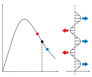
One of the most intriguing predictions of the sandpaper theory, supported by roughness-resolving simulations, is the non-monotonic pattern of the roughness-induced drag. For relatively slow abyssal flows, drag increases with rising speed. However, when currents reach a certain velocity, bottom drag begins to decrease, as illustrated in figure 1. This reduction is attributed to the homogenization of net potential vorticity in the abyssal layer, which occurs at high flow speeds and partially offsets the topographic form drag (Radko Reference Radko2022a,Reference Radkob). The dissimilar patterns of the conventional and the sandpaper drag laws are not particularly surprising. These models address very different physical processes operating on disparate spatial scales. Nevertheless, the relatively new proposition that the bottom-drag law may be non-monotonic prompts an inquiry into its large-scale ramifications. This concern becomes particularly urgent since forcing induced by rough topography can easily dominate the local turbulent drag for representative conditions (e.g. Radko Reference Radko2022a,Reference Radkob). In particular, the present study explores the connection between the non-monotonic drag-law pattern and the instability of large-scale abyssal flows.

Figure 1. Schematic diagram illustrating (a) the non-monotonic forcing pattern produced by rough topography and (b) the physical mechanism of the drag-law instability. A decrease in the bottom drag  $(\varPhi )$ with increasing velocity (u) results in the growth of perturbations $u^{\prime} = u - U$ of a uniform zonal current of speed U.
The physical argument pointing to a potentially destabilizing tendency of seafloor roughness is illustrated in figure 1. Consider a steady zonal current with uniform speed U flowing above rough topography. This current is assumed to be maintained by the external basin-scale forcing that balances the bottom drag in the integral sense. Suppose this current's speed is large enough to place it on the decreasing limb of the drag law  $\varPhi$(u). The basic state $\{ U,\varPhi (U)\}$ is indicated on the diagram in figure 1(a) by the black dot. Consider a weak, zonally uniform perturbation $u^{\prime}(y) = u - U$ that increases the zonal velocity (u) in some locations but decreases it in others. Relatively swift parts of the flow (blue dot in figure 1a) would experience a reduction in the bottom drag. Since external mechanisms maintain the mean flow strength, these water masses will likely respond to the drag reduction by accelerating further, as indicated by the blue arrows in figure 1(b). Relatively slow flows (red dot in figure 1a), on the other hand, would be affected by larger bottom drag and therefore will likely decelerate. Thus, the perturbations will amplify in time, implying the instability of uniform flows.
There are obvious parallels between the proposed mechanism of drag-law instability and the well-known instability of buoyancy flux laws (Phillips Reference Phillips1972; Posmentier Reference Posmentier1977; Balmforth, Llewellyn Smith & Young Reference Balmforth, Llewellyn Smith and Young1998). The latter models consider the evolution of turbulent density-stratified systems and conclude that states with uniform stratification are inherently unstable if the vertical eddy-induced buoyancy flux decreases with increasing buoyancy gradient. It was suggested that the flux-law instability may induce the spontaneous formation of mixed layers separated by thin interfaces – an effect reproduced in laboratory experiments with turbulent one-component flows (Ruddick, McDougall & Turner Reference Ruddick, McDougall and Turner1989; Park, Whitehead & Gnanadeskian Reference Park, Whitehead and Gnanadeskian1994). If the analogy between the flux-law and drag-law instabilities extends into the nonlinear regime, it is conceivable that the latter will result in a state dominated by swift parallel jets, interspersed by relatively quiescent water masses. One of the principal objectives of this study is to determine whether, and to what degree, this evolutionary outcome is realized for typical oceanic conditions.
The material is organized as follows. In § 2, we consider the homogeneous quasi-geostrophic model in which the effects of rough topography are represented by non-monotonic drag laws based on the sandpaper theory. The obtained parametric solutions are compared with the corresponding terrain-resolving simulations. Section 3 extends the analysis to stratified systems using a two-layer isopycnal model. The results are summarized, and conclusions are drawn, in § 4.
2. The homogeneous model
2.1. Formulation
The minimal framework for the analysis of the interaction of large-scale barotropic flows with topography is the quasi-geostrophic rigid-lid model (e.g. Pedlosky Reference Pedlosky1987)
 \begin{equation}\frac{{\partial {\nabla ^2}\varPsi }}{{\partial t}} + J(\varPsi ,{\nabla ^2}\varPsi ) + \beta \frac{{\partial \varPsi }}{{\partial x}} + \frac{{{f_0}}}{{{H_0}}}J(\varPsi ,\eta ) = \upsilon {\nabla ^4}\varPsi - \gamma {\nabla ^2}\varPsi ,\end{equation}
where  $\varPsi $ is the streamfunction associated with the velocity field $(u,v) = ( - \partial \varPsi /\partial y, \partial \varPsi /\partial x)$, $\eta $ is the depth variation, J is the Jacobian, $\upsilon $ is the lateral eddy viscosity, $\gamma $ is the Ekman bottom-drag coefficient and $\beta \equiv \partial f/\partial y$ is the meridional gradient of planetary vorticity. The constant reference values of the ocean depth and the Coriolis parameters are denoted by ${H_0}$ and ${f_0}$, respectively. It should be noted that typical large-scale interior oceanic flows, far separated from the coastal boundaries, tend to be zonally oriented. To reflect this property, the net streamfunction $(\varPsi )$ is separated into the basic state representing the uniform zonal current $( - Uy)$ and the perturbation $(\psi )$ for which we assume doubly periodic boundary conditions. When the governing equation (2.1) is expressed in terms of $\psi$, we arrive at
 \begin{align}\frac{{\partial {\nabla ^2}\psi }}{{\partial t}} + J(\psi ,{\nabla ^2}\psi ) + U\frac{{\partial {\nabla ^2}\psi }}{{\partial x}} + \beta \frac{{\partial \psi }}{{\partial x}} + \frac{{{f_0}}}{{{H_0}}}J(\psi ,\eta ) + U\frac{{\partial \eta }}{{\partial x}} = \upsilon {\nabla ^4}\psi - \gamma {\nabla ^2}\psi .\end{align}
The pattern of rough topography  $(\eta )$ is constructed using the empirical spectrum derived by Goff & Jordan (Reference Goff and Jordan1988) from the echo-sounding ocean depth sampling
 \begin{equation}{P_h} = \frac{{\eta _0^2(\mu - 2)}}{{{{(2{{\rm \pi} })}^3}{k_0}{l_0}}}{\left( {1 + {{\left( {\frac{k}{{2{{\rm \pi} }{k_0}}}} \right)}^2} + {{\left( {\frac{l}{{2{{\rm \pi} }{l_0}}}} \right)}^2}} \right)^{ - \mu /2}},\end{equation}
where k and l are the zonal and meridional wavenumbers respectively, and the coefficient  ${\eta _0}$ controls the root-mean-square roughness amplitude $({\eta _{rms}})$. In the present study, we assume parameters suggested by Nikurashin et al. (Reference Nikurashin, Ferrari, Grisouard and Polzin2014)
 \begin{equation}\mu = 3.5,\quad {k_0} = 1.8 \times {10^{ - 4}}\;{\textrm{m}^{ - 1}},\quad {l_0} = 1.8 \times {10^{ - 4}}\;{\textrm{m}^{ - 1}},\end{equation}
and represent bottom topography by a sum of Fourier modes with random phases and spectral amplitudes conforming to the Goff–Jordan spectrum.
The present study also considers the sandpaper model of roughness (Radko Reference Radko2023a,Reference Radkob, Reference Radko2024). Its key result is the explicit large-scale evolutionary equation that, in the present framework, takes the form
 \begin{equation}\frac{{\partial {\nabla ^2}{\psi _{ls}}}}{{\partial t}} + J({\psi _{ls}},{\nabla ^2}{\psi _{ls}}) + U\frac{{\partial {\nabla ^2}{\psi _{ls}}}}{{\partial x}} + \beta \frac{{\partial {\psi _{ls}}}}{{\partial x}} + curl\,\boldsymbol{F} = \upsilon {\nabla ^4}{\psi _{ls}} - \gamma {\nabla ^2}{\psi _{ls}},\end{equation}
where  ${\psi _{ls}}$ is the large-scale perturbation streamfunction and F denotes the roughness-induced drag
 \begin{equation}\boldsymbol{F} = \varPhi ({V_{abs}})\boldsymbol{s},\quad \varPhi = \sqrt {{G_{slow}}{G_{fast}}}\, exp ( - \sqrt {1 + {{[\ln ({V_{abs}}V_C^{ - 1})]}^2}} ).\end{equation}
In this expression,  $\boldsymbol{s} = ({u_{ls}} + U,{v_{ls}})V_{abs}^{ - 1}$ denotes the unit vector aligned in the direction of the large-scale flow $({u_{ls}} + U,{v_{ls}})$ and ${V_{abs}} = \sqrt {{{({u_{ls}} + U)}^2} + v_{ls}^2}$. Model (2.6) is designed to bridge two distinct regimes. For relatively slow flows $({V_{abs}} \ll {V_C})$ the forcing magnitude increases with large-scale velocity $\varPhi \approx {G_{slow}}{V_{abs}}$. However, this forcing begins to decrease with increasing speed $(\varPhi \approx {G_{fast}}V_{abs}^{ - 1})$ when the flow is sufficiently swift $({V_{abs}} \gg {V_C})$, as illustrated by the schematic diagram in figure 1(a). The critical velocity marking the transition between fast-flow and slow-flow regimes is given by ${V_C} = \sqrt {{G_{fast}}/{G_{slow}}} $, where coefficients ${G_{fast}}$ and ${G_{slow}}$ are determined by the roughness pattern. In its most basic form, the sandpaper theory (e.g. Radko Reference Radko2023b) suggests
 \begin{equation}{G_{fast}} = 2{{\rm \pi} }\upsilon \frac{{f_0^2}}{{H_0^2}}\int {|\tilde{\eta }{|^2}\kappa \,\textrm{d}\kappa } ,\quad {G_{slow}} = \frac{{{\rm \pi} }}{\upsilon }\frac{{f_0^2}}{{H_0^2}}\int {|\tilde{\eta }{|^2}{\kappa ^{ - 1}}\,\textrm{d}\kappa } ,\quad \kappa = \sqrt {{k^2} + {l^2}} ,\end{equation}
where  $\tilde{\eta }(\kappa )$ is the Fourier image of rough bathymetry, which is assumed to be isotropic and restricted to a finite range of wavelengths
 \begin{equation}{L_{min}} < 2{{\rm \pi} }{\kappa ^{ - 1}} < {L_{max}}.\end{equation}
The upper limit is imposed to permit a distinct treatment of small scales that we wish to parameterize, and large scales incorporated explicitly in the model. The lower bound in (2.8) is introduced to ensure that the Rossby numbers remain uniformly small, as required by the quasi-geostrophic model (2.2). In the following calculations, we assume  ${L_{min}} = 3\;\textrm{km}$ and ${L_{max}} = 30\;\textrm{km}$.
2.2. Linear stability analysis
Our starting point is the stability analysis of the parametric large-scale vorticity equation (2.5). The uniform basic flow  $({\psi _{ls}} = 0)$ represents an exact solution of (2.5), and its linearization in the limit of weak perturbations $(|{\psi _{ls}}|\to 0)$ yields
 \begin{equation}\frac{{\partial {\nabla ^2}{\psi _{ls}}}}{{\partial t}} + U\frac{{\partial {\nabla ^2}{\psi _{ls}}}}{{\partial x}} + \beta \frac{{\partial {\psi _{ls}}}}{{\partial x}} + {\varPhi _1}\frac{{{\partial ^2}{\psi _{ls}}}}{{\partial {y^2}}} + \frac{{{\varPhi _0}}}{{|U|}}\frac{{{\partial ^2}{\psi _{ls}}}}{{\partial {x^2}}} = \upsilon {\nabla ^4}{\psi _{ls}} - \gamma {\nabla ^2}{\psi _{ls}},\end{equation}
where
 \begin{equation}{\varPhi _0} = \varPhi \textrm{(}U\textrm{),}\quad {\varPhi _1} = {\left. {\frac{{\partial \varPhi }}{{\partial {V_{abs}}}}} \right|_{{V_{abs}} = U}}.\end{equation}
We consider normal modes
 \begin{equation}{\psi _{ls}} = \hat{\psi }exp (\textrm{i}kx + ily + \lambda t),\end{equation}
which reduce (2.9) to
 \begin{equation}\lambda ={-} \textrm{i}Uk + \textrm{i}\beta k{\kappa ^{ - 2}} - \upsilon {\kappa ^2} - {\varPhi _1}{l^2}{\kappa ^{ - 2}} - {\varPhi _0}|U{|^{ - 1}}{k^2}{\kappa ^{ - 2}} - \gamma .\end{equation}
 Of particular interest is the real part of the growth rate  $({\lambda _r})$, which determines the stability of the basic state
 \begin{equation}{\lambda _r} ={-} \upsilon {\kappa ^2} - {\varPhi _1}{l^2}{\kappa ^{ - 2}} - {\varPhi _0}|U{|^{ - 1}}{k^2}{\kappa ^{ - 2}} - \gamma .\end{equation}
It should be emphasized that the only potentially destabilizing factor in this system is the second term on the right-hand side of (2.13), which is determined by the pattern of the roughness-induced drag law. If this drag decreases with the increasing velocity  $({\varPhi _1} < 0)$, positive growth rates are possible. This conclusion is consistent with the physical interpretation of the drag-law instability in figure 1.
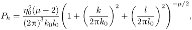
In figure 2, we plot the growth rate  ${\lambda _r}$ as a function of wavenumbers for the oceanographically representative parameters of
 \begin{equation}\begin{split}f &= {10^{ - 4}}\;{\textrm{s}^{ - 1}},\quad \beta = 2 \times {10^{ - 11}}\;{\textrm{m}^{ - 1}}\;{\textrm{s}^{ - 1}},\quad \gamma = 2 \times {10^{ - 7}}\;{\textrm{s}^{ - 1}},\\ \upsilon &= 20\;{\textrm{m}^{ - 1}}\;{\textrm{s}^{ - 1}},\quad {\eta _{rms}} = 300\;\textrm{m,}\quad {H_0} = 3000\;\textrm{m}\textrm{.}\end{split}\end{equation}
The results in figure 2 indicate that the growth rates are of the order of  ${\lambda _r}\sim {10^{ - 7}}\;{\textrm{s}^{ - 1}}$, which corresponds to the amplification periods of approximately a hundred days. Another notable finding is that the largest growth rates are realized for modes with $k = 0$, which suggests that the drag-law instability likely takes the form of parallel zonal jets. For zonally uniform modes, ${\lambda _r}$ monotonically increases with the decreasing meridional wavenumber, and $l = 0$ represents a singular point in the growth rate pattern. This implies that linear stability analysis cannot predict the preferred meridional scale of drag-law instabilities.
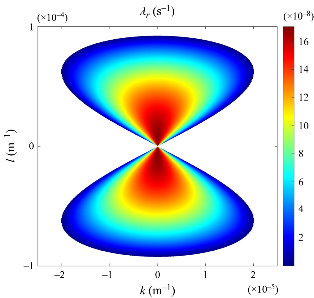
Figure 2. The growth rates  $({\lambda _r})$ predicted by linear stability analysis are plotted as a function of the wavenumbers k and l. Only positive growth rates are shown.
2.3. Nonlinear parametric model
To glean insight into the nonlinear dynamics of drag-law instability, we integrate the parametric model (2.5) numerically. The simulation is performed using the de-aliased pseudo-spectral model employed in our previous studies (e.g. Radko Reference Radko2022a,Reference Radkob) on the computational domain of size  $({L_x},{L_y}) = (2 \times {10^6}\;\textrm{m},\;{10^6}\;\textrm{m})$ resolved by $({N_x},{N_y}) = (512,256)$ grid points. Other model parameters are listed in (2.14). The experiment is initiated by the random low-amplitude distribution of ${\psi _{ls}}$, introduced to seed primary instabilities. It is extended for ten years of model time, and the results are presented in figure 3. The left panels show the patterns of vorticity ${\varsigma _{ls}} = {\nabla ^2}{\psi _{ls}}$ at various times, and the x-averaged zonal velocity $\langle u\rangle$ is plotted as a function of y in the right panels.

Figure 3. The parametric simulation. The instantaneous large-scale vorticity patterns  $({\varsigma _{ls}})$ are potted at $t = 1,3$ and 10 years in panels (a,c,e), respectively. Panels (b,d,f) show the corresponding patterns of the x-averaged zonal velocity $\langle u\rangle$.
The first stage in the development of the drag-law instability is the emergence of weak and relatively narrow striations, shown in figure 3(a,b) at  $t = 1$ year. These structures are predominantly zonal. Their limited meridional extent is attributed to the random initial distribution of ${\psi _{ls}}$, which preferentially excites small (grid-scale) perturbations. However, in time, jets amplify and merge. These mergers tend to occur when relatively strong jets grow at the expense of weaker ones, which gradually disappear. No systematic meridional drift is observed. Using the nomenclature introduced by Radko (Reference Radko2007), these evolutionary patterns can be described as B-mergers. By $t = 3$ years (figure 3c,d), the flow field becomes dominated by thin, high-shear interfaces separated by much wider low-shear zones. Such patterns are reminiscent of – and perhaps dynamically analogous to – the so-called potential vorticity staircases. The latter can form in turbulent fluids due to the suppression of eddy transport across the potential vorticity barriers (Baldwin et al. Reference Baldwin, Rhines, Huang and McIntyre2007; Dritschel & McIntyre Reference Dritschel and McIntyre2008). Finally, by $t = 10$ years (figure 3e,f), the system evolves into a quasi-steady state consisting of two isolated zonal jets.
2.4. Roughness-resolving simulation
The parametric calculations (§§ 2.2 and 2.3) are highly suggestive in describing key features of the drag-law instability. However, a more stringent and convincing test of our ideas is afforded by the roughness-resolving simulation. The following model integrates the full vorticity equation (2.2) and does not attempt to introduce the drag laws a priori. The pattern of topography conforms to the Goff–Jordan spectrum (2.3). The requirement to resolve rough topography demands using a much finer grid, and therefore we adopt a mesh with  $({N_x},{N_y}) = (4096,2048)$ grid points. Other parameters match those used for the parametric simulation in figure 3.
The roughness-resolving simulation is shown in figure 4. Due to its interaction with small-scale topography, the flow rapidly develops fine structures. In particular, the vorticity field  $\varsigma = {\nabla ^2}\psi $ becomes completely dominated by variability on scales of several kilometres. To reveal the underlying large-scale vorticity pattern, we apply Gaussian smoothing with the filtering scale of ${L_{max}} = 30\;\textrm{km}$, and the resulting large-scale vorticity $({\varsigma _{ls}})$ patterns are presented in figure 4(a,c,e). The evolution of the flow field in the roughness-resolving simulation is broadly consistent with that in figure 3. The first evolutionary phase is characterized by the emergence of numerous zonally oriented jets (figure 4a,b), which strengthen and occasionally merge (figure 4c,d). By $t = 10$ years (figure 4e,f) the system reaches statistical equilibrium represented by two well-defined jets separated by relatively slow flows.

Figure 4. The same as in figure 3, but for the roughness-resolving simulation.
There are some visible differences between the parametric (figure 3) and roughness-resolving (figure 4) simulations. For instance, in the roughness-resolving experiment, topography rapidly generates substantial perturbations to the basic current, and therefore the transition to the fully nonlinear regime is more rapid. By  $t = 1$ year, the perturbation velocity (figure 4b) is already comparable to the mean. In the parametric simulation, the perturbation at the same stage is still very weak (figure 3b). The vorticity fronts in the roughness-resolving experiment are wider – whereas the maximal velocity of jets is somewhat lower – than in the parametric simulation. Nevertheless, the general similarities in the evolution of these two systems are undeniable, which instils confidence in our interpretation of the dynamics at play in both roughness-resolving and parametric models.
3. The stratified model
3.1. Formulation
Our next step toward realism is the analysis of the drag-law instability in a stratified system. We use the two-layer quasi-geostrophic model (e.g. Pedlosky Reference Pedlosky1987). In each layer, we separate the streamfunction  ${\varPsi _{\,i}}(i = 1,2)$ into the basic state representing a uniform zonal current $( - {U_i}y)$ and the perturbation $({\psi _i})$, which reduces the governing equations to
 \begin{equation}\left. \begin{aligned}
&{\dfrac{{\partial {q_1}}}{{\partial t}} +
J({\psi_1},{q_1}) + \left( {\beta + \dfrac{{{U_1} -
{U_2}}}{{R_{d\,1}^2}}} \right)\dfrac{{\partial
{\psi_1}}}{{\partial x}} + {U_1}\dfrac{{\partial
{q_1}}}{{\partial x}} = \upsilon {\nabla^4}{\psi_1}}\\
&\dfrac{{\partial {q_2}}}{{\partial t}} + J({\psi_2},{q_2})
+ \dfrac{{{f_0}}}{{{H_2}}}J({\psi_2},\eta ) +
{U_2}\dfrac{{\partial \eta }}{{\partial x}} + \left( {\beta
+ \dfrac{{{U_2} - {U_1}}}{{R_{d\,2}^2}}}
\right)\dfrac{{\partial {\psi_2}}}{{\partial x}} +
{U_2}\dfrac{{\partial {q_2}}}{{\partial x}}\\&\quad =
\upsilon {\nabla^4}{\psi_2} - \gamma {\nabla^2}{\psi_2}
\end{aligned}
\right\},\end{equation}
\begin{equation}\left. \begin{aligned}
&{\dfrac{{\partial {q_1}}}{{\partial t}} +
J({\psi_1},{q_1}) + \left( {\beta + \dfrac{{{U_1} -
{U_2}}}{{R_{d\,1}^2}}} \right)\dfrac{{\partial
{\psi_1}}}{{\partial x}} + {U_1}\dfrac{{\partial
{q_1}}}{{\partial x}} = \upsilon {\nabla^4}{\psi_1}}\\
&\dfrac{{\partial {q_2}}}{{\partial t}} + J({\psi_2},{q_2})
+ \dfrac{{{f_0}}}{{{H_2}}}J({\psi_2},\eta ) +
{U_2}\dfrac{{\partial \eta }}{{\partial x}} + \left( {\beta
+ \dfrac{{{U_2} - {U_1}}}{{R_{d\,2}^2}}}
\right)\dfrac{{\partial {\psi_2}}}{{\partial x}} +
{U_2}\dfrac{{\partial {q_2}}}{{\partial x}}\\&\quad =
\upsilon {\nabla^4}{\psi_2} - \gamma {\nabla^2}{\psi_2}
\end{aligned}
\right\},\end{equation}
where  ${R_{\,di}} = \sqrt {g^{\prime}{H_i}} /{f_0}$ is the radius of deformation of layer i, ${H_i}$ is the layer thickness, $g^{\prime}$ is the reduced gravity and ${q_i}$ is the perturbation potential vorticity
 \begin{equation}\left.
{\begin{array}{*{20}{c}} {{q_1} = {\nabla^2}{\psi_1} +
\dfrac{{{\psi_2} - {\psi_1}}}{{R_{d\,1}^2}}}\\ {{q_2} =
{\nabla^2}{\psi_1} + \dfrac{{{\psi_1} -
{\psi_2}}}{{R_{d\,2}^2}}} \end{array}}
\right\}.\end{equation}
\begin{equation}\left.
{\begin{array}{*{20}{c}} {{q_1} = {\nabla^2}{\psi_1} +
\dfrac{{{\psi_2} - {\psi_1}}}{{R_{d\,1}^2}}}\\ {{q_2} =
{\nabla^2}{\psi_1} + \dfrac{{{\psi_1} -
{\psi_2}}}{{R_{d\,2}^2}}} \end{array}}
\right\}.\end{equation}In the following calculations, we assume
 \begin{equation}{H_1} = 1000\;\textrm{m},\quad {H_2} = 3000\;\textrm{m},\quad g^{\prime} = 0.01\;{\textrm{m}^2}\;{\textrm{s}^{ - 1}},\end{equation}
while other parameters are assigned the same values as in the homogeneous model (2.14). In parametric calculations based on the sandpaper theory, the governing equations for large-scale flow components are
 \begin{equation}\left. \begin{aligned}
&{\dfrac{{\partial {q_{ls\,1}}}}{{\partial t}} +
J({\psi_{ls\,1}},{q_{ls\,1}}) + \left( {\beta + \dfrac{{{U_1} -
{U_2}}}{{R_{d\,1}^2}}} \right)\dfrac{{\partial
{\psi_{ls\,1}}}}{{\partial x}} + {U_1}\dfrac{{\partial
{q_{ls\,1}}}}{{\partial x}} = \upsilon
{\nabla^4}{\psi_{ls\,1}}}\\ &\dfrac{{\partial
{q_{ls\,2}}}}{{\partial t}} + J({\psi_{ls\,2}},{q_{ls\,2}}) +
\left( {\beta + \dfrac{{{U_2} - {U_1}}}{{R_{d\,2}^2}}}
\right)\dfrac{{\partial {\psi_{ls\,2}}}}{{\partial x}} +
{U_2}\dfrac{{\partial {q_{ls\,2}}}}{{\partial x}} +
curl\,\boldsymbol{F}\\ &\quad = \upsilon
{\nabla^4}{\psi_{ls\,2}} - \gamma {\nabla^2}{\psi_{ls\,2}}
\end{aligned}
\right\}.\end{equation}
\begin{equation}\left. \begin{aligned}
&{\dfrac{{\partial {q_{ls\,1}}}}{{\partial t}} +
J({\psi_{ls\,1}},{q_{ls\,1}}) + \left( {\beta + \dfrac{{{U_1} -
{U_2}}}{{R_{d\,1}^2}}} \right)\dfrac{{\partial
{\psi_{ls\,1}}}}{{\partial x}} + {U_1}\dfrac{{\partial
{q_{ls\,1}}}}{{\partial x}} = \upsilon
{\nabla^4}{\psi_{ls\,1}}}\\ &\dfrac{{\partial
{q_{ls\,2}}}}{{\partial t}} + J({\psi_{ls\,2}},{q_{ls\,2}}) +
\left( {\beta + \dfrac{{{U_2} - {U_1}}}{{R_{d\,2}^2}}}
\right)\dfrac{{\partial {\psi_{ls\,2}}}}{{\partial x}} +
{U_2}\dfrac{{\partial {q_{ls\,2}}}}{{\partial x}} +
curl\,\boldsymbol{F}\\ &\quad = \upsilon
{\nabla^4}{\psi_{ls\,2}} - \gamma {\nabla^2}{\psi_{ls\,2}}
\end{aligned}
\right\}.\end{equation}
The explicit expression for the roughness-induced drag F is still given by (2.6) and (2.7), albeit in the multilayer model, it is based on the characteristics of the bottom layer:  ${H_0} \to {H_2}$ and ${\boldsymbol{v}_{ls}} \to {\boldsymbol{v}_{ls\,2}}$.
3.2. Barotropic background flow
Our starting point for the analysis of the stratified system is the barotropic background flow with  ${U_1} = {U_2} = 0.05\;\textrm{m}\;{\textrm{s}^{ - 1}}$. This case offers an opportunity to examine the influence of density stratification on drag-law instability in isolation from the effects that can be attributed to the background shear. The latter will be considered in § 3.3.
The linear stability analysis proceeds in the same manner as in the homogeneous models (§ 2.2). We linearize the large-scale equations (3.4) and assume normal modes
 \begin{equation}{\psi _{ls\;i}} = {\hat{\psi }_i}exp (\textrm{i}kx + ily + \lambda t),\quad i = 1,2,\end{equation}
which yields the quadratic eigenvalue equation for the growth rate. We focus on the root with the larger real component  $({\lambda _r})$, which is plotted as a function of wavenumbers $(k,l)$ in figure 5. The growth rate pattern in figure 5 is structurally similar to its homogeneous counterpart (figure 2). The largest growth rates are still attained by the zonally oriented $(k = 0)$ modes, although the values of ${\lambda _r}$ tend to be somewhat lower. Thus, while stratification adversely affects the drag-law instability, it does not completely suppress it.
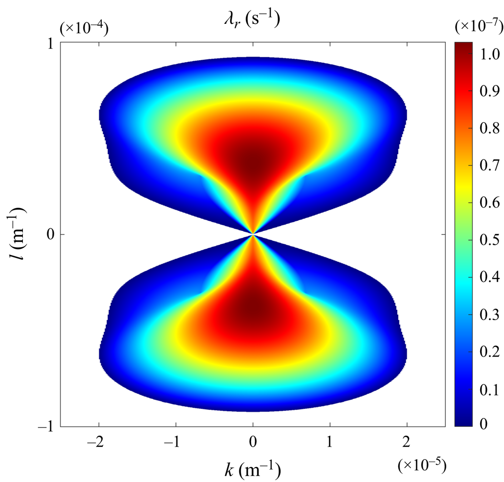
Figure 5. The growth rates  $({\lambda _r})$ predicted by linear stability analysis are plotted as a function of wavenumbers k and l for the two-layer model with the barotropic background flow. Only positive growth rates are shown.
A principal difference between the stratified growth rate pattern and its homogeneous counterpart (figure 2) is related to the location of maximal  ${\lambda _r}$. The growth rate in figure 5 is maximized at a finite meridional wavenumber $({l_{max}} ={\pm} 3.7 \times {10^{ - 5}}\;{\textrm{m}^{ - 1}})$. In contrast, the homogeneous growth rate increases with decreasing $|l|$, but the maximal value cannot be attained because of the model's singularity at $l = 0$. We attribute this dissimilar behaviour to the presence of the intrinsic and dynamically significant length scales in the stratified model that are set by deformation radii $({R_{\,di}})$. These scales have no counterpart in the homogeneous system (2.5). Another interesting feature of figure 5 is the abrupt variation in the growth rate pattern at $(k,l) = ({\pm} 7 \times {10^{ - 6}}, \pm 3 \times {10^{ - 5}})\;{\textrm{m}^{ - 1}}$. At these locations, the discriminant of the quadratic eigenvalue equation is zero. Therefore, such points mark transitions between structurally dissimilar branches of the solution.
The nonlinear evolutionary patterns of the drag-law instability in the stratified and homogeneous models are analogous. This conclusion is based on stratified simulations, the resolution, model parameters and the numerical algorithm of which match those used in § 2. In figure 6, we present the potential vorticity patterns realized in the simulation of the parametric system (3.4) at  $t = 1,5$ and 15 years. While the development and equilibration of instability in the stratified system in figure 6 is slower than in its homogeneous counterpart (figure 3), it goes through the same basic stages. First, we observe the formation of multiple narrow striations that are particularly apparent in the second-layer potential vorticity field (figure 6a). These structures undergo a series of binary mergers, which increase their width (figure 6c). The system eventually evolves into a quasi-equilibrium state in which thin high-q interfaces are separated by much broader zones with low potential vorticity (figure 6e). The flow patterns observed in the upper layer (figure 6b,d,e) are structurally similar to – but considerably weaker than – the structures in the abyssal ocean (figure 6a,c,e).
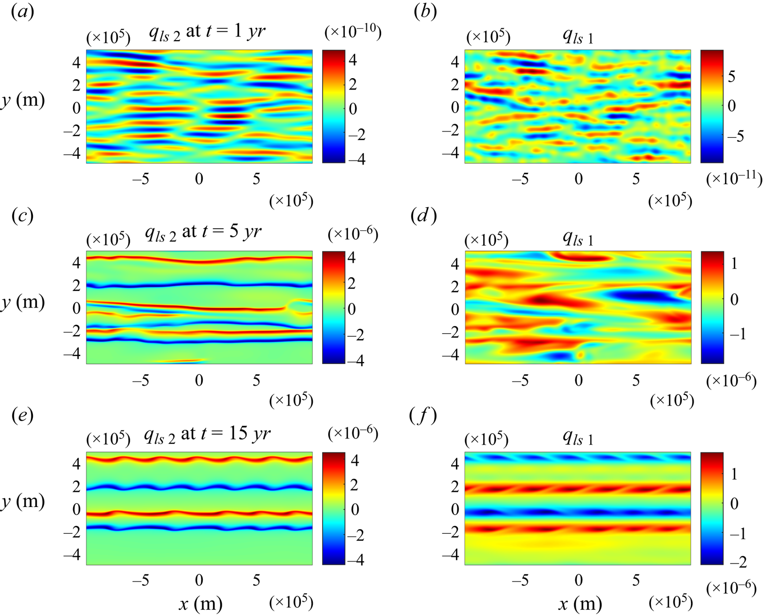
Figure 6. The parametric simulation. The instantaneous large-scale potential vorticity patterns in the abyssal layer  $({q_{ls\,2}})$ are potted at $t = 1,5$ and 15 years in panels (a,c,e), respectively. Panels (b,d,f) show the corresponding patterns of potential vorticity in the upper layer $({q_{ls\,1}})$.
Figure 7 presents the roughness-resolving simulation of the full quasi-geostrophic system (3.1). The potential vorticity in the second layer is dominated by kilometre-scale variability induced by rough topography. To reveal the underlying large-scale pattern, we smooth  ${q_2}$ with the filtering scale of ${L_{max}} = 30\;\textrm{km}$. The resulting patterns of large-scale vorticity $({q_{ls\,2}})$ are presented in figure 7(a,c,e) at $t = 1,5$ and 15 years. The potential vorticity in the upper layer is largely devoid of small-scale variability, and therefore we present (figure 7b,d,f) the unaltered pattern of ${q_1}$. The evolutionary patterns realized in this experiment are broadly consistent with both parametric simulation (figure 6) and its homogeneous roughness-resolving counterpart (figure 4). Once again, we first observe the development of narrow weak striations (figure 7a,b), which strengthen and merge (figure 7c,d), and then equilibrate (figure 7e,f). The similar development of drag-law instability in various configurations indicates that our conclusions are sufficiently robust and general.

Figure 7. The same as in figure 6 but for the roughness-resolving simulation.
3.3. Baroclinic background flow
The configuration that we explore next is distinguished by the presence of substantial vertical shear
 \begin{equation}{U_1} = 0.1\;\textrm{m}\;{\textrm{s}^{ - 1}},\quad {U_2} = 0.05\;\textrm{m}\;{\textrm{s}^{ - 1}}.\end{equation}
All other parameters are the same as in § 3.2. In terms of mean velocity pattern and orientation, this system broadly reflects characteristics of the Antarctic Circumpolar Current – a major zonal oceanic flow that circumnavigates the globe in the Southern Ocean (e.g. Johnson & Bryden Reference Johnson and Bryden1989; Hallberg & Gnanadesikan Reference Hallberg and Gnanadesikan2006). The key dynamic consequence of vertical shear in the ocean is baroclinic instability. Thus, this model makes it possible to gain insight into the interaction of the baroclinic and drag-law instabilities.
In this regard, linear stability analysis of the parametrized system (3.4) proves to be informative. In figure 8(a), we plot the growth rates  $({\lambda _r})$ realized for the baroclinic background flow (3.6) as a function of k and l. The central unstable region shaped as number 8 in the wavenumber space closely matches the pattern realized for the barotropic flow (figure 5) and therefore is attributed to the drag-law instability. However, in figure 8(a) we also see unstable side lobes that are absent in figure 5. These features are interpreted as the manifestation of baroclinic instability. This suggestion is further reinforced by the calculation in figure 8(b), which presents the flat-bottom counterpart of the growth rate pattern in figure 8(a). Excluding the roughness-induced drag (F = 0), eliminates the 8-shaped pattern at the centre but retains the side lobes. It should be noted that roughness substantially increases the growth rates of baroclinic instability. The tendency of baroclinic instability to intensify in response to dissipative processes has been discussed previously in the context of Ekman friction (e.g. Swaters Reference Swaters2010). The fact that it is realized for a considerably different roughness-induced drag model points to the generic nature of dissipation-induced destabilization. A series of growth rate calculations analogous to those in figure 8 have also been performed with numerous other values of $({U_1},{U_2})$. These analyses consistently indicate that, while the vertical shear $({U_1} - {U_2})$ controls the growth rate of baroclinic instability, it has only a marginal impact on drag-law instabilities. The latter are largely determined by the abyssal flow (U 2).

Figure 8. The growth rates  $({\lambda _r})$ predicted by linear stability analysis are plotted as a function of wavenumbers k and l for the two-layer model with the baroclinic background flow. The calculation in (a) is performed for the root mean square roughness amplitude of ${\eta _{rms}} = 300\;\textrm{m}$, whereas the corresponding flat-bottom calculation $({\eta _{rms}} = 0\textrm{)}$ is shown in panel (b). Only positive growth rates are shown.
The following examples focus on the nonlinear evolution of drag-law instability in parametric (figure 9) and topography-resolving (figures 10 and 11) simulations. The key feature brought by the presence of a baroclinic background flow is the intense mesoscale variability, clearly identifiable in potential vorticity patterns (figures 9 and 10). The irregular transient eddies, which we attribute to baroclinic instability, are particularly active in the upper layer. Although mesoscale variability partially masks the zonal jets, they are still visible. The plots of the x-averaged velocity (figure 11) are particularly revealing in this regard. In both upper and lower layers, weak and relatively narrow jets form first (figure 11a,b), intensify and merge (figure 11c,d) and eventually settle into a quasi-equilibrium state (figure 11e,f). Note that the upper- and lower-layer jets remain spatially well correlated throughout the simulation. This implies that the drag-law instability is particularly effective in controlling the barotropic component of the flow field.
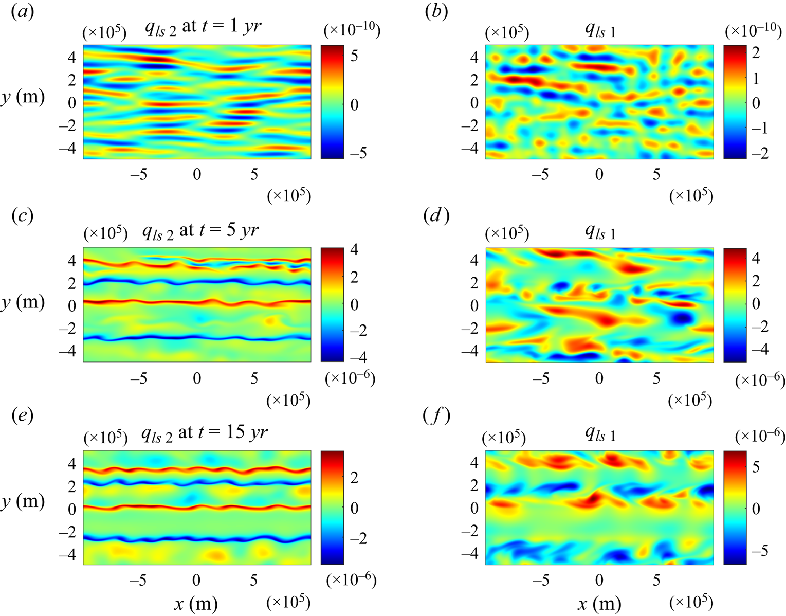
Figure 9. The same as in figure 6 but for the baroclinic background flow.

Figure 10. The same as in figure 9 but for the roughness-resolving simulation.

Figure 11. The roughness-resolving simulation. The instantaneous patterns of the x-averaged zonal velocity in the upper (right panels) and lower (left panels) layers are potted as a function of y at  $t = 1,5$ and 15 years in the first, second and third rows of panels, respectively.
4. Discussion
This study explores the instabilities of large-scale ocean currents caused by irregular kilometre-scale bathymetric variability. Such patterns are ubiquitous in the World Ocean and are commonly referred to as seafloor roughness. Although the general theory of flow interaction with rough topography is still in its infancy (Mashayek Reference Mashayek2023; Radko Reference Radko2023a,Reference Radkob, Reference Radko2024), recent studies reveal some generic and reproducible tendencies. Notably, there is an emerging consensus regarding the profound impact of roughness on large-scale circulation patterns (e.g. LaCasce et al. Reference LaCasce, Escartin, Chassignet and Xu2019; Chassignet & Xu Reference Chassignet and Xu2021; Gulliver & Radko Reference Gulliver and Radko2022). The forcing of abyssal currents by rough topography likely surpasses the drag induced by small-scale turbulence in the bottom boundary layer, which has been used almost exclusively to represent the flow–seafloor interaction in the past.
The non-monotonic pattern of bottom drag is another consistent characteristic of rough topography (Gulliver & Radko Reference Gulliver and Radko2023; Radko Reference Radko2023a,Reference Radkob, Reference Radko2024). For relatively slow flows, drag increases with the speed of abyssal currents but, after reaching a critical velocity, it starts to decrease (figure 1a). According to the sandpaper theory (Radko Reference Radko2023a), this non-monotonic pattern reflects two distinct physical mechanisms of roughness-induced forcing. Slow flows are primarily affected by the form drag, which arises from pressure differences upstream and downstream of topographic features. Fast flows, on the other hand, are more susceptible to the Reynolds stresses associated with eddies generated by rough terrain. This forcing pattern represents a cardinal departure from the traditional oceanographic models, which assume monotonic – either linear or quadratic – drag laws. It is worth noting that an analogous reduction in the air–sea drag coefficient at high wind speeds has been reported in the meteorological literature (e.g. Powel et al. Reference Powell, Vickery and Reinhold2003). However, the frictional mechanisms in the lower atmosphere are substantially different from those proposed by the sandpaper theory for the abyssal flows in the ocean.
The relatively new suggestion that the bottom drag can decrease with increasing flow speed prompts an inquiry into its large-scale consequences. Of particular concern is the possibility of destabilization of abyssal currents, and the suggested mechanism of drag-law instability is illustrated in figure 1. We assume that the mean flow strength is maintained by basin-scale processes of unspecified origin. In this case, the local increase in speed of relatively swift currents is accompanied by the reduction in bottom drag, further accelerating the flow. Conversely, the speed reduction implies higher drag, which slows down the flow even more, and this positive feedback points to the instability of large-scale currents.
The linear stability analyses and numerical simulations in this study confirm our suspicions. Fast, laterally uniform flows develop instabilities in the form of zonal jets separated by relatively quiescent zones. These structures appear in both stratified and homogeneous systems. Although mesoscale variability, caused by the baroclinic instability of the background flow, makes these jets less prominent, they can still be readily identified by zonally averaging the velocity fields (figure 11). Importantly, drag-law instabilities develop even in roughness-resolving simulations that make no a priori assumptions about the relation between bottom forcing and flow speed. It should be noted that the present model considers zonal background currents, which reflects the predominant orientation of large-scale flows in the ocean interior. Thus, the zonal orientation of drag-law instabilities could be caused by the direction of the background flow or by the meridional variation of the Coriolis parameter. The relative contribution of these effects is not clear at this point and could be regime dependent.
The instability signatures extend throughout the entire water column even in stratified simulations. Therefore, it is possible that drag-law instabilities, particularly the most intense ones, can be detected in satellite-based sea surface measurements. The patterns forming in our experiments resemble zonal striations commonly observed in the ocean (Maximenko, Bang & Sasaki Reference Maximenko, Bang and Sasaki2005; Sokolov & Rintoul Reference Sokolov and Rintoul2007; Maximenko et al. Reference Maximenko, Melnichenko, Niiler and Sasaki2008; Berloff & Kamenkovich Reference Berloff and Kamenkovich2019). The alternating zonal jets can be generated by several mechanisms (e.g. Senior, Zhai & Stevens Reference Senior, Zhai and Stevens2024), and they have also been identified in simulations that do not resolve seafloor roughness (e.g. Kamenkovich, Berloff & Pedlosky Reference Kamenkovich, Berloff and Pedlosky2009). Nevertheless, the tendency of drag-law instability to preferentially amplify zonal patterns indicates that it can promote the formation and maintenance of oceanic striations.
The present investigation can be extended in several ways. Perhaps the most pressing next step is the search for observational confirmation of our ideas. The suggested non-monotonicity of drag laws and the associated destabilization of large-scale flows are based on theoretical arguments and idealized numerical models. Consequently, many processes that could interfere with the proposed mechanisms in the ocean are excluded from the outset. Another promising avenue of inquiry lies in theoretical explorations of the nonlinear evolution of such systems. It is crucial to fully explain the dynamics of jet-merging events and the statistical equilibration of drag-law instabilities. There are several precedents for the analytical treatment of quasi-one-dimensional systems that could guide such studies (e.g. Manfroi & Young Reference Manfroi and Young1999). For instance, it may be prudent to exploit the analogy between the drag-law instability and the more extensively studied Phillips–Posmentier instability of turbulent flux laws (e.g. Balmforth et al. Reference Balmforth, Llewellyn Smith and Young1998; Radko Reference Radko2007; Pružina, Hughes & Pegler Reference Pružina, Hughes and Pegler2023). The analysis of drag-law instabilities in non-zonal background flows is also bound to reveal a rich and interesting dynamics. In all such endeavours, the present study can serve as necessary proof of concept and a starting point for more detailed investigations.
Acknowledgements
The author thanks the editor N. Balmforth and the anonymous reviewers for helpful comments.
Funding
This work was supported by the National Science Foundation (grant OCE 2241625) and the Office of Naval Research (grant N00014-24-WX-01685).
Declaration of interests
The author reports no conflict of interest.


