1 INTRODUCTION
Accurate description of the properties at the crust–core interface of neutron stars (NS) is crucial for correct interpretation of a wide range of astrophysical phenomena such as glitches and X-ray bursts. However, modelling neutron stars across their entire range of densities within the same framework is a big challenge, as different types of matter appear at different density regimes. The composition of the outer crust for isolated NSs is given by the ground state of matter below the neutron drip density (roughly ρ ≃ 4 × 10¹¹ g cm−3). According to the cold catalysed matter hypothesis, matter is in full thermodynamic equilibrium at zero temperature. At the surface, the outer crust consists of a lattice of iron nuclei. As the density increases, the composition of the nuclei becomes more and more neutron rich as a result of electron capture. Beyond the neutron drip density, the inner crust consists of neutron-rich clusters in a gas of electrons and free neutrons.
In general, different theoretical models are applied to describe separately the homogeneous matter in the core and the clusterised matter in the crust. The outer crust is assumed to be composed of perfect crystals with one representative nuclear species at lattice sites (bcc), embedded in a sea of electrons. Each lattice volume is represented by a Wigner–Seitz cell, assumed to be charge neutral and in chemical equilibrium. The determination of the composition of the outer crust is largely sensitive to the experimentally determined nuclear masses (Baym et al. Reference Baym, Pethick and Sutherland1971a; Salpeter Reference Salpeter1961). Terrestrial nuclear physics experiments may help to constrain the composition of the subsaturation matter in the outer crust, but in the inner crust, the neutron-rich nuclei are far away from the valley of stability and hence beyond the reach of nuclear experiments. Thus, for the description of the inner crust, one needs to resort to theoretical models for the extrapolation to higher densities. Some commonly used techniques are Compressible Liquid Drop model (Baym, Bethe, & Pethick Reference Baym, Bethe and Pethick1971b; Douchin & Haensel Reference Douchin and Haensel2001), Hartree–Fock/Hartree–Fock Bogoliubov (Negele & Vautherin Reference Negele and Vautherin1973; Grill, Margueron, & Sandulescu Reference Grill, Margueron and Sandulescu2011), Extended Thomas–Fermi approximation (Onsi et al. Reference Onsi, Dutta, Chatri, Goriely, Chamel and Pearson2008), etc.
Usually, the crust–core matching is done in a way that the pressure is always an increasing function of density. However, it was demonstrated recently (Fortin et al. Reference Fortin, Providência, Raduta, Gulminelli, Zdunik, Haensel and Bejger2016) that the use of non-unified models at the crust–core boundary leads to arbitrary results, with an uncertainty in the crust thickness of up to 30% and up to 4% for the estimation of the radius. Further the non-unified models show no or spurious correlations with experimentally determined observables such as symmetry energy and its derivatives, as demonstrated in the works by Khan & Margueron (Reference Khan and Margueron2013) and Ducoin et al. (Reference Ducoin, Margueron, Providência and Vidaña2011).
One of the main challenges for nuclear theory is therefore to develop unified models that are able to reproduce both clusterised matter in nuclei in the crust on one hand, and homogeneous matter in the core on the other, within the same formalism. Despite the huge recent advancement in methodological and numerical techniques, ab-initio approaches, which derive properties of nuclei from the underlying nuclear forces, are limited to relatively light nuclei (as far as 48Ca) (Hagen et al. Reference Hagen2016). An alternative approach is by employing the nuclear energy density functional (EDF) method. There has been tremendous success in application of the density functional theory (DFT) for the description of non-relativistic many particle systems. DFT calculations involve solving a system of non-interacting particles, which interact through a self-consistent effective potential that could be relativistic (Relativistic Mean Field) or non-relativistic (employing local Skyrme or non-local Gogny potentials). The parameters of the density functionals are optimised to selected experimental data and known properties of homogeneous nuclear matter (HNM). However, there is no one-to-one correlation between the parameters of the functional and the physical properties of nuclear matter, implying that the constraints obtained on nuclear matter are still model dependent.
There are quite a few experimental observables that serve to constrain the nuclear Equation of State (EoS) at subsaturation densities (Fortin et al. Reference Fortin, Providência, Raduta, Gulminelli, Zdunik, Haensel and Bejger2016), such as neutron-skin thickness, heavy ion collisions, electric dipole polarisability, Giant Dipole Resonances (GDR) of neutron-rich nuclei, measurement of nuclear masses, isobaric analog states, etc. Of these, the weak charge form factor, neutron skins, dipole polarisability, etc. are good indicators of the isovector dependence, while giant resonance energies, isoscalar and isovector effective masses, incompressibility and saturation density are weakly dependent on asymmetry.
In this work, we use a recently proposed (Margueron, Casali, & Gulminelli Reference Margueron, Casali and Gulminelli2017a, Reference Margueron, Casali and Gulminelli2017b) empirical EoS for HNM for the neutron star core, that incorporates the most recent empirical knowledge of nuclear experimental observables. The functional, when extended to non-homogeneous matter in finite nuclei, contains more parameters that take into account surface properties and spin-orbit effects, but still the one-to-one correspondence between model parameters and EoS empirical parameters is kept. Recently, an analytical mass formula was developed (Aymard, Gulminelli, & Margueron Reference Aymard, Gulminelli and Margueron2016a, Reference Aymard, Gulminelli and Margueron2016b; Aymard, Gulminelli, & Margueron Reference Aymard, Gulminelli and Margueron2014) based on the analytical integration of the Skyrme functional in the ETF approximation. In this study, we will utilise this analytical formula to describe finite nuclei, but we use the empirical functional instead of the Skyrme parametrisation. We will show that one requires, in addition to the empirical coefficients, only one extra effective parameter to obtain a reasonable description of nuclear masses, bypassing the more sophisticated and rigorous full ETF calculations. The advantage of this minimal formalism is that one is able to single out the influence of the EoS parameters.
2 FORMALISM
2.1. Unified description of the NS crust and core
Using the DFT, the energy density of a nuclear system can be expressed as an algebraic function of densities such as nucleon density, kinetic energy density, spin-orbit densities, etc., and their gradients:
 $$\begin{equation}
{\cal {H}} = {\cal {H}} [\rho _q (\vec{r}), \nabla _{q^{\prime }}^k \rho _q (\vec{r})].
\end{equation}$$
$$\begin{equation}
{\cal {H}} = {\cal {H}} [\rho _q (\vec{r}), \nabla _{q^{\prime }}^k \rho _q (\vec{r})].
\end{equation}$$
The ground state can then be determined by minimisation of energy, and the parameters of the functional optimised to reproduce certain selected observables of finite nuclei (such as experimental nuclear mass, charge radii) and of nuclear matter (saturation properties). In general, there can be an infinite number of gradients in the functional. In the case of HNM, the functional consists only of density terms (k = 0), the so-called Thomas–Fermi approximation. For finite nuclei, restricting non-zero number of gradient terms up to k in the expansion results in the so-called kth order ETF approach. The advantage of this approach is that the energy density of a nuclear system can be calculated if the neutron and proton densities are given in a parametrised form. This allows the development of an analytical mass formula (Aymard et al. Reference Aymard, Gulminelli and Margueron2016a, Reference Aymard, Gulminelli and Margueron2016b; Aymard et al. Reference Aymard, Gulminelli and Margueron2014), to link directly the form of the functional and the parameters of the interaction in the ETF approximation. In this study, we employ this analytical mass formula for the calculation of the energies in the ETF approximation. We describe this in detail in the following section.
2.2. Empirical EoS for NS core: Homogeneous matter
We describe the energy density of homogeneous matter by an ‘Empirical’ EoS, whose parameters are related directly to nuclear observables. The energy per particle in asymmetric nuclear matter can be separated into isoscalar and isovector channels, as
 $$\begin{equation}
e(\rho ,\delta ) = e_{\text{IS}}(\rho ) + \delta ^2 e_{\text{IV}}(\rho ).
\end{equation}$$
$$\begin{equation}
e(\rho ,\delta ) = e_{\text{IS}}(\rho ) + \delta ^2 e_{\text{IV}}(\rho ).
\end{equation}$$
Here, δ = (ρ p − ρ n )/ρ is the asymmetry of bulk nuclear matter, the density ρ being the sum of proton and neutron densities ρ p and ρ n , respectively. The empirical parameters appear as the coefficients of the series expansion around saturation density ρsat in terms of a dimensionless parameter x = (ρ − ρsat)/3ρsat, i.e.,
 $$\begin{equation}
e_{IS} = E_{{\rm sat}} + \frac{1}{2} K_{{\rm sat}} x^2 + \frac{1}{3!} Q_{{\rm sat}} x^3 + \frac{1}{4!} Z_{{\rm sat}} x^4
\end{equation}$$\\
$$\begin{equation}
e_{IS} = E_{{\rm sat}} + \frac{1}{2} K_{{\rm sat}} x^2 + \frac{1}{3!} Q_{{\rm sat}} x^3 + \frac{1}{4!} Z_{{\rm sat}} x^4
\end{equation}$$\\
 $$\begin{equation}
e_{IV} = E_{{\rm sym}} + L_{{\rm sym}} x + \frac{1}{2} K_{{\rm sym}} x^2 + \frac{1}{3!} Q_{{\rm sym}} x^3 +\, \frac{1}{4!} Z_{{\rm sym}} x^4 .
\end{equation}$$
$$\begin{equation}
e_{IV} = E_{{\rm sym}} + L_{{\rm sym}} x + \frac{1}{2} K_{{\rm sym}} x^2 + \frac{1}{3!} Q_{{\rm sym}} x^3 +\, \frac{1}{4!} Z_{{\rm sym}} x^4 .
\end{equation}$$
The isoscalar channel is written in terms of the energy per particle at saturation E sat, the isoscalar incompressibility K sat, the skewness Q sat, etc. The isovector channel is defined in terms of the symmetry energy E sym and its derivatives L sym, K sym, etc. In principle, there is an infinite number of terms in the series expansion. However, it was shown (Margueron et al. Reference Margueron, Casali and Gulminelli2017a, Reference Margueron, Casali and Gulminelli2017b) that for nuclear densities less than 0.2 fm−3, the convergence of the expansion is achieved already at the second order in x. Therefore, in this study that is limited to finite nuclei, i.e., subsaturation densities, we restrict the expansion up to to second order.
In the development of the empirical EoS, to account for the correct isospin dependence beyond the parabolic approximation, the density dependence of the kinetic energy term is separated from that of the potential term:
 $$\begin{equation}
e (x,\delta ) = e_{\text{kin}} (x,\delta ) + e_{{\rm pot}} (x,\delta ).
\end{equation}$$
$$\begin{equation}
e (x,\delta ) = e_{\text{kin}} (x,\delta ) + e_{{\rm pot}} (x,\delta ).
\end{equation}$$
The kinetic energy term is given by the Fermi gas expression:
 $$\begin{equation}
e_{\text{kin}} = t_0^{\text{FG}} (1+3 x)^{2/3} \frac{1}{2} \left[ (1+\delta )^{5/3} \frac{m}{m_n^*} + (1-\delta )^{5/3}\frac{m}{m_p^*} \right],
\end{equation}$$
$$\begin{equation}
e_{\text{kin}} = t_0^{\text{FG}} (1+3 x)^{2/3} \frac{1}{2} \left[ (1+\delta )^{5/3} \frac{m}{m_n^*} + (1-\delta )^{5/3}\frac{m}{m_p^*} \right],
\end{equation}$$
where the constant
 $t_0^{\text{FG}}$
is given by
$t_0^{\text{FG}}$
is given by
 $$\begin{equation}
t_0^{\text{FG}} = \frac{3}{5}\frac{\hbar ^2}{2m} \left( \frac{3 \pi ^2}{2} \right)^{2/3} \rho _{{\rm sat}}^{2/3},
\end{equation}$$
$$\begin{equation}
t_0^{\text{FG}} = \frac{3}{5}\frac{\hbar ^2}{2m} \left( \frac{3 \pi ^2}{2} \right)^{2/3} \rho _{{\rm sat}}^{2/3},
\end{equation}$$
where ℏ and m are the usual reduced Planck’s constant and inertial nucleon mass, respectively. However, the interaction in nuclear matter modifies the inertial mass of the nucleons. The in-medium effective mass m* q for a nucleon q = n, p can be expanded in terms of the density parameter x as
 $$\begin{equation}
\frac{m}{m^*_q} = \sum _{\alpha =0}^1 m_{\alpha }^q (\delta ) \frac{x^{\alpha }}{\alpha !}.
\end{equation}$$
$$\begin{equation}
\frac{m}{m^*_q} = \sum _{\alpha =0}^1 m_{\alpha }^q (\delta ) \frac{x^{\alpha }}{\alpha !}.
\end{equation}$$
For asymmetric nuclear matter, we can define two parameters to characterise the in-medium effective mass:
 $$\begin{eqnarray}
\bar{m} = m_0^q (\delta =0) - 1, \nonumber \\
\bar{\Delta } = \frac{1}{2} [m_0^n(\delta =1)-m_0^p(\delta =1)].
\end{eqnarray}$$
$$\begin{eqnarray}
\bar{m} = m_0^q (\delta =0) - 1, \nonumber \\
\bar{\Delta } = \frac{1}{2} [m_0^n(\delta =1)-m_0^p(\delta =1)].
\end{eqnarray}$$
Here,
 $\bar{\Delta }$
is the isospin splitting of the nucleon masses. The effective mass in nuclear medium can then be expressed as
$\bar{\Delta }$
is the isospin splitting of the nucleon masses. The effective mass in nuclear medium can then be expressed as
 $$\begin{equation}
\frac{m}{m_q^*} = 1 + (\bar{m} + \tau _{3q} \: \bar{\Delta }\delta ) (1+3x),
\end{equation}$$
$$\begin{equation}
\frac{m}{m_q^*} = 1 + (\bar{m} + \tau _{3q} \: \bar{\Delta }\delta ) (1+3x),
\end{equation}$$
where τ3q is the Pauli vector ( = 1 for neutrons and −1 for protons).
Similarly, we may write the potential part of the energy per particle as a Taylor series expansion separated into isoscalar and isovector contributions a α0 and a α2, up to second order in the parameter x as follows (Margueron et al. Reference Margueron, Casali and Gulminelli2017a, Reference Margueron, Casali and Gulminelli2017b):
 $$\begin{equation}
e_{{\rm pot}} = \sum _{\alpha =0}^2 (a_{\alpha 0} + a_{\alpha 2} \delta ^2) \frac{x^{\alpha }}{\alpha !} u_{\alpha } (x),
\end{equation}$$
$$\begin{equation}
e_{{\rm pot}} = \sum _{\alpha =0}^2 (a_{\alpha 0} + a_{\alpha 2} \delta ^2) \frac{x^{\alpha }}{\alpha !} u_{\alpha } (x),
\end{equation}$$
where the form of the correction factor u α(x) = 1 − ( − 3x)3 e −b(3x + 1) is chosen such that the energy per particle goes to zero at ρ = 0. The parameter b is determined by imposing that the value of the exponential function is 1/2 at ρ = 0.1ρsat, giving b = 10ln 2.
Comparing with Equations (3) and (4), the isoscalar coefficients in the expansion can be written in terms of the known empirical parameters:
 $$\begin{equation}
a_{00} = E_{{\rm sat}} - t_0^{FG} ( 1 + \bar{m}),
\end{equation}$$\\
$$\begin{equation}
a_{00} = E_{{\rm sat}} - t_0^{FG} ( 1 + \bar{m}),
\end{equation}$$\\
 $$\begin{equation}
a_{10} = - t_0^{FG} ( 2 + 5 \bar{m}),
\end{equation}$$\\
$$\begin{equation}
a_{10} = - t_0^{FG} ( 2 + 5 \bar{m}),
\end{equation}$$\\
 $$\begin{equation}
a_{20} = K_{{\rm sat}} - 2 t_0^{FG} ( 5 \bar{m} - 1),
\end{equation}$$
$$\begin{equation}
a_{20} = K_{{\rm sat}} - 2 t_0^{FG} ( 5 \bar{m} - 1),
\end{equation}$$
and similarly for the isovector coefficients in the expansion
 $$\begin{equation}
a_{02} = E_{{\rm sym}} - \frac{5}{9} t_0^{FG} ( 1 + (\bar{m}+3{\bar{\Delta }})),
\end{equation}$$\\
$$\begin{equation}
a_{02} = E_{{\rm sym}} - \frac{5}{9} t_0^{FG} ( 1 + (\bar{m}+3{\bar{\Delta }})),
\end{equation}$$\\
 $$\begin{equation}
a_{12} = L_{{\rm sym}} - \frac{5}{9} t_0^{FG} ( 2 + 5(\bar{m}+3{\bar{\Delta }})),
\end{equation}$$\\
$$\begin{equation}
a_{12} = L_{{\rm sym}} - \frac{5}{9} t_0^{FG} ( 2 + 5(\bar{m}+3{\bar{\Delta }})),
\end{equation}$$\\
 $$\begin{equation}
a_{22} = K_{{\rm sym}} - \frac{10}{9} t_0^{FG} ( -1 + 5(\bar{m}+3{\bar{\Delta }})).
\end{equation}$$
$$\begin{equation}
a_{22} = K_{{\rm sym}} - \frac{10}{9} t_0^{FG} ( -1 + 5(\bar{m}+3{\bar{\Delta }})).
\end{equation}$$
The present uncertainty in empirical parameters (see Table 1) was compiled recently from a large number of Skyrme, Relativistic Mean Field and Relativistic Hartree–Fock models (Margueron et al. Reference Margueron, Casali and Gulminelli2017a, Reference Margueron, Casali and Gulminelli2017b) and their average and standard deviation were estimated. It may be noted from Table 1 that the saturation density and energy/particle at saturation are very well constrained. The uncertainties of incompressibility, symmetry energy and its first derivative lie within a relatively small interval, while for higher derivatives of the symmetry energy the uncertainty is large.
Table 1. Empirical parameters obtained from various effective approaches (Margueron et al. Reference Margueron, Casali and Gulminelli2017a).

2.3. Inhomogeneous matter in NS crust: Finite nuclei
Given a parametrised density profile ρ(r), the energy of a spherical nucleus can be determined using the ETF energy functional
 $$\begin{equation}
E = \int dr {\cal {H}}_{{\rm ETF}} [\rho (r)].
\end{equation}$$
$$\begin{equation}
E = \int dr {\cal {H}}_{{\rm ETF}} [\rho (r)].
\end{equation}$$
The mean field potential for the nucleons inside the atomic nucleus can be described by a Woods–Saxon potential. A reasonable choice for the neutron and proton density profiles (q = n, p) is ρ q (r) = ρ0q F(r), with the Fermi function defined as F(r) = (1 + e (r − Rq )/aq )− 1. The parameters ρ q and R q are obtained by fitting the Fermi function to Hartree–Fock calculations (Papakonstantinou et al. Reference Papakonstantinou, Margueron, Gulminelli and Raduta2013): ρ0q = ρ0(δ)(1 ± δ)/2. In the above expression, the saturation density for asymmetric nuclei depends on the asymmetry δ and can be written as (Papakonstantinou et al. Reference Papakonstantinou, Margueron, Gulminelli and Raduta2013)
 $$\begin{equation}
\rho _{0} (\delta ) = \rho _{{\rm sat}} \left( 1 - \frac{3 L_{{\rm sym}}}{K_{{\rm sat}} + K_{{\rm sym}} \delta ^2} \right).
\end{equation}$$
$$\begin{equation}
\rho _{0} (\delta ) = \rho _{{\rm sat}} \left( 1 - \frac{3 L_{{\rm sym}}}{K_{{\rm sat}} + K_{{\rm sym}} \delta ^2} \right).
\end{equation}$$
In addition, one needs to make the hypothesis that both neutron and protons have the same diffuseness of the density profile, i.e., a n = a p = a. The diffuseness a can then be determined by the minimisation of the energy, i.e., ∂E/∂a = 0.
One can choose to work with any two parametrised density profiles: here, we choose the total density ρ(r) and proton density profile ρ p (r) (Aymard et al. Reference Aymard, Gulminelli and Margueron2016b):
 $$\begin{equation}
\rho (r) = \rho _{0} F(r)
\end{equation}$$
$$\begin{equation}
\rho (r) = \rho _{0} F(r)
\end{equation}$$
and
 $$\begin{equation}
\rho _p(r) = \rho _{0p} F_p(r).
\end{equation}$$
$$\begin{equation}
\rho _p(r) = \rho _{0p} F_p(r).
\end{equation}$$
The saturation densities are related by the bulk asymmetry:
 $$\begin{equation}
\delta = 1 - 2 \frac{\rho _{0p}}{\rho _{0}}.
\end{equation}$$
$$\begin{equation}
\delta = 1 - 2 \frac{\rho _{0p}}{\rho _{0}}.
\end{equation}$$
The bulk asymmetry differs from the global asymmetry I = 1 − 2Z/A, as is evident from the relation obtained from the droplet model (Myers & Swiatecki Reference Myers and Swiatecki1980; Centelles, Del Estal, & Viñas Reference Centelles, Del Estal and Viñas1998; Warda et al. Reference Warda, Viñas, Roca-Maza and Centelles2009)
 $$\begin{equation}
\delta = \frac{I + \frac{3 a_c Z^2}{8 Q A^{5/3}} }{1 + \frac{9 J_{{\rm sym}}}{4 Q A^{1/3}} },
\end{equation}$$
$$\begin{equation}
\delta = \frac{I + \frac{3 a_c Z^2}{8 Q A^{5/3}} }{1 + \frac{9 J_{{\rm sym}}}{4 Q A^{1/3}} },
\end{equation}$$
where ac is the Coulomb parameter and Q is the surface stiffness parameter. In finite nuclei, in addition to the bulk contribution E b , there are contributions to the energy from the finite size, i.e., surface effects E s :
 $$\begin{equation*}
E(A,\delta ) = E_b(A,\delta ) + E_s(A,\delta ) .\nonumber
\end{equation*}$$
$$\begin{equation*}
E(A,\delta ) = E_b(A,\delta ) + E_s(A,\delta ) .\nonumber
\end{equation*}$$
The bulk energy is the energy of a homogeneous nuclear matter without finite size effects
 $$\begin{equation}
E_b(A,\delta ) = E_{{\rm sat}} A,
\end{equation}$$
$$\begin{equation}
E_b(A,\delta ) = E_{{\rm sat}} A,
\end{equation}$$
where E sat(δ) = e(x, δ) is the energy per particle of asymmetric homogeneous nuclear matter defined in Equation (5), calculated at the saturation density of asymmetric nuclear matter, x = (ρ0(δ) − ρsat)/3ρsat. The surface energy can be decomposed into an isoscalar-like part, where the isospin dependence only comes from the variation of the saturation density with the isospin parameter δ, and an explicitly isovector part, which accounts for the residual isospin dependence:
 $$\begin{equation*}
E_s(A,\delta ) = E_s^{\text{IS}}(A,\delta ) + E_s^{\text{IV}}(A,\delta )\delta ^2 .\nonumber
\end{equation*}$$
$$\begin{equation*}
E_s(A,\delta ) = E_s^{\text{IS}}(A,\delta ) + E_s^{\text{IV}}(A,\delta )\delta ^2 .\nonumber
\end{equation*}$$
Both isoscalar and isovector terms of the surface energy E s contain contributions from the gradient terms in the energy functional. These can be separated into local and non-local terms:
 $$\begin{equation*}
E_s = E_s^L + E_s^{\text{NL}}. \nonumber
\end{equation*}$$
$$\begin{equation*}
E_s = E_s^L + E_s^{\text{NL}}. \nonumber
\end{equation*}$$
The local terms, which depend only on the density, can be expressed directly in terms of the EoS parameters. The non-local terms arise from the gradient terms in the functional, such as the finite size term C
fin(∇ρ)2 + D
fin(∇ρ3)2, spin-orbit term
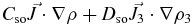 $C_{\text{so}}\vec{J} \cdot \nabla \rho + D_{\text{so}}\vec{J}_3 \cdot \nabla \rho _3$
, spin gradient term
$C_{\text{so}}\vec{J} \cdot \nabla \rho + D_{\text{so}}\vec{J}_3 \cdot \nabla \rho _3$
, spin gradient term
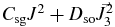 $C_{\text{sg}} J^2 + D_{\text{so}}\vec{J}_3^2$
, etc. (here, ρ3 = ρδ is the isovector particle density and J and J
3 are the isoscalar and isovector spin-orbit density vectors, see Aymard et al. Reference Aymard, Gulminelli and Margueron2016b).
$C_{\text{sg}} J^2 + D_{\text{so}}\vec{J}_3^2$
, etc. (here, ρ3 = ρδ is the isovector particle density and J and J
3 are the isoscalar and isovector spin-orbit density vectors, see Aymard et al. Reference Aymard, Gulminelli and Margueron2016b).
Allowing analytic integration of Fermi functions, the local isoscalar surface energy can be decomposed into a plane surface, curvature and higher order terms (Aymard et al. Reference Aymard, Gulminelli and Margueron2016b):
 $$\begin{eqnarray}
E_s^{\text{IS},L} &=& {\cal {C}}^L_{{\rm surf}} \frac{a(A)}{r_{0}} A^{2/3} \nonumber \\
&&+\, {\cal {C}}^L_{{\rm curv}} \left[ \frac{a(A)}{r_{0}} \right]^2 A^{1/3} \nonumber \\
&&+\, {\cal {C}}^L_{{\rm ind}} \left[ \frac{a(A)}{r_{0}} \right]^3 ,
\end{eqnarray}$$
$$\begin{eqnarray}
E_s^{\text{IS},L} &=& {\cal {C}}^L_{{\rm surf}} \frac{a(A)}{r_{0}} A^{2/3} \nonumber \\
&&+\, {\cal {C}}^L_{{\rm curv}} \left[ \frac{a(A)}{r_{0}} \right]^2 A^{1/3} \nonumber \\
&&+\, {\cal {C}}^L_{{\rm ind}} \left[ \frac{a(A)}{r_{0}} \right]^3 ,
\end{eqnarray}$$
where
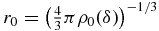 $r_{0}= \left(\frac{4}{3}\pi \rho _{0}(\delta )\right)^{-1/3}$
, and the expressions for the coefficients
$r_{0}= \left(\frac{4}{3}\pi \rho _{0}(\delta )\right)^{-1/3}$
, and the expressions for the coefficients
 ${\cal {C}}(\delta )$
have been defined in Aymard et al. (Reference Aymard, Gulminelli and Margueron2016a, Reference Aymard, Gulminelli and Margueron2016b). The coefficients depend only on the EoS parameters. For the non-local surface energy
${\cal {C}}(\delta )$
have been defined in Aymard et al. (Reference Aymard, Gulminelli and Margueron2016a, Reference Aymard, Gulminelli and Margueron2016b). The coefficients depend only on the EoS parameters. For the non-local surface energy
 $E_s^{\text{IS},\text{NL}}$
:
$E_s^{\text{IS},\text{NL}}$
:
 $$\begin{eqnarray}
E_s^{\text{IS},\text{NL}} = \frac{1}{a^2(A)} {\cal {C}}^{\text{NL}}_{{\rm surf}} \frac{a(A)}{r_{0}} A^{2/3} \nonumber \\
+\, \frac{1}{a^2(A)} {\cal {C}}^{\text{NL}}_{{\rm curv}} \left[ \frac{a(A)}{r_{0}} \right]^2 A^{1/3} \nonumber \\
+\, \frac{1}{a^2(A)} {\cal {C}}^{\text{NL}}_{{\rm ind}} \left[ \frac{a(A)}{r_{0}} \right]^3 .
\end{eqnarray}$$
$$\begin{eqnarray}
E_s^{\text{IS},\text{NL}} = \frac{1}{a^2(A)} {\cal {C}}^{\text{NL}}_{{\rm surf}} \frac{a(A)}{r_{0}} A^{2/3} \nonumber \\
+\, \frac{1}{a^2(A)} {\cal {C}}^{\text{NL}}_{{\rm curv}} \left[ \frac{a(A)}{r_{0}} \right]^2 A^{1/3} \nonumber \\
+\, \frac{1}{a^2(A)} {\cal {C}}^{\text{NL}}_{{\rm ind}} \left[ \frac{a(A)}{r_{0}} \right]^3 .
\end{eqnarray}$$
The non-local coefficients defined in Aymard et al. (Reference Aymard, Gulminelli and Margueron2016a, Reference Aymard, Gulminelli and Margueron2016b) depend on EoS parameters and also on two additional finite-size parameters C fin and C so. In order to isolate the influence of the EoS parameters, we propose a single ‘effective’ parameter C fin for the finite size effects. We constrain this parameter in the next section using experimental nuclear observables.
The decomposition of the surface energy into isoscalar and isovector parts is not straight-forward, since both terms have an implicit dependence on the asymmetry δ. If the explicit isovector term
 $E_s^{\text{IV}}$
is ignored, the diffuseness a
IS can be variationally obtained by solving
$E_s^{\text{IV}}$
is ignored, the diffuseness a
IS can be variationally obtained by solving
 $\frac{\partial E_s}{\partial a}=0$
, giving the following estimation for the diffuseness:
$\frac{\partial E_s}{\partial a}=0$
, giving the following estimation for the diffuseness:
 $$\begin{eqnarray}
3 \mathcal {C}_{{\rm ind}}^{L} \left( \frac{a_{\text{IS}}}{r_{0}} \right)^4 + 2 \mathcal {C}_{{\rm curv}}^{L} A^{1/3} \left( \frac{a_{\text{IS}}}{r_{0}} \right)^3 \nonumber\\
+ \left( \mathcal {C}_{{\rm surf}}^{L} A^{2/3} + \frac{1}{r_{0}^2} \mathcal {C}_{{\rm ind}}^{\text{NL}} \right) \left( \frac{a_{\text{IS}}}{r_{0}} \right)^2 - \frac{1}{r_{0}^2} \mathcal {C}_{{\rm surf}}^{\text{NL}} A^{2/3} = 0 .
\end{eqnarray}$$
$$\begin{eqnarray}
3 \mathcal {C}_{{\rm ind}}^{L} \left( \frac{a_{\text{IS}}}{r_{0}} \right)^4 + 2 \mathcal {C}_{{\rm curv}}^{L} A^{1/3} \left( \frac{a_{\text{IS}}}{r_{0}} \right)^3 \nonumber\\
+ \left( \mathcal {C}_{{\rm surf}}^{L} A^{2/3} + \frac{1}{r_{0}^2} \mathcal {C}_{{\rm ind}}^{\text{NL}} \right) \left( \frac{a_{\text{IS}}}{r_{0}} \right)^2 - \frac{1}{r_{0}^2} \mathcal {C}_{{\rm surf}}^{\text{NL}} A^{2/3} = 0 .
\end{eqnarray}$$
If one neglects the curvature and A-independent terms, one obtains the simple solution for ‘slab’ geometry:
 $$\begin{equation}
a_{{\rm slab}} = \sqrt{\frac{{\cal {C}}^{\text{NL}}_{{\rm surf}}}{{\cal {C}}^L_{{\rm surf}}} }.
\end{equation}$$
$$\begin{equation}
a_{{\rm slab}} = \sqrt{\frac{{\cal {C}}^{\text{NL}}_{{\rm surf}}}{{\cal {C}}^L_{{\rm surf}}} }.
\end{equation}$$
We can see from this simple equation that in the limit of purely local energy functional, the optimal configuration would be a homogeneous hard sphere a = 0. The presence of non-local terms in the functional results in finite diffuseness for atomic nuclei.
The total diffuseness a must however include the isovector contribution. Unfortunately, the isovector surface part cannot be written as simple integrals of Fermi functions (since the isovector density ρ − ρ
p
is not a Fermi function). Hence, it cannot be integrated analytically to evaluate
 $E_s^{\text{IV}}$
, and one requires approximations to develop an analytical expression. Following Aymard et al. (Reference Aymard, Gulminelli and Margueron2016b), we assume that the isovector energy density can be approximated by a Gaussian peaked at r = R:
$E_s^{\text{IV}}$
, and one requires approximations to develop an analytical expression. Following Aymard et al. (Reference Aymard, Gulminelli and Margueron2016b), we assume that the isovector energy density can be approximated by a Gaussian peaked at r = R:
 $$\begin{equation}
{\cal {H}}_s^{\text{IV}}(r) = {\cal {A}}(A,\delta ) e^{-\frac{(r-R)^2}{2 \sigma ^2(A,\delta )} },
\end{equation}$$
$$\begin{equation}
{\cal {H}}_s^{\text{IV}}(r) = {\cal {A}}(A,\delta ) e^{-\frac{(r-R)^2}{2 \sigma ^2(A,\delta )} },
\end{equation}$$
where
 ${\cal {A}}$
is the maximum amplitude of the Gaussian distribution and σ is the variance at R. The isovector surface energy
${\cal {A}}$
is the maximum amplitude of the Gaussian distribution and σ is the variance at R. The isovector surface energy
 $E_s^{\text{IV}}$
in the Gaussian approximation can be written in terms of a surface contribution and a contribution independent of A:
$E_s^{\text{IV}}$
in the Gaussian approximation can be written in terms of a surface contribution and a contribution independent of A:
 $$\begin{equation}
E_s^{\text{IV}} = E_{{\rm surf}}^{\text{IV}} A^{2/3} + E_{{\rm ind}}^{\text{IV}},
\end{equation}$$
$$\begin{equation}
E_s^{\text{IV}} = E_{{\rm surf}}^{\text{IV}} A^{2/3} + E_{{\rm ind}}^{\text{IV}},
\end{equation}$$
(see Aymard et al. Reference Aymard, Gulminelli and Margueron2016b for the full equations and detailed derivation). The total diffuseness can then be determined by mimimising the energy with respect to the diffuseness parameter a, i.e.,
 $\frac{\partial E}{\partial a} = 0$
. In the Gaussian approximation is then given by Aymard et al. (Reference Aymard, Gulminelli and Margueron2016b):
$\frac{\partial E}{\partial a} = 0$
. In the Gaussian approximation is then given by Aymard et al. (Reference Aymard, Gulminelli and Margueron2016b):
 $$\begin{eqnarray}
&& a^2 (A,\delta) = a_{IS}^2 (\delta) \nonumber \\
&+& \sqrt{\frac{\pi}{(1-\frac{K_{1/2}}{18 J_{1/2}})}} \frac{\rho_{sat}}{\rho_{0}(\delta)}
\frac{3 J_{1/2}(\delta-\delta^2)}{{\cal{C}}^L_{surf}(\delta)} a_{slab} \Delta R_{HS} (A,\delta).
\end{eqnarray}$$
$$\begin{eqnarray}
&& a^2 (A,\delta) = a_{IS}^2 (\delta) \nonumber \\
&+& \sqrt{\frac{\pi}{(1-\frac{K_{1/2}}{18 J_{1/2}})}} \frac{\rho_{sat}}{\rho_{0}(\delta)}
\frac{3 J_{1/2}(\delta-\delta^2)}{{\cal{C}}^L_{surf}(\delta)} a_{slab} \Delta R_{HS} (A,\delta).
\end{eqnarray}$$
In this expression, the coefficients J
1/2, K
1/2 represent the value of the symmetry energy and its curvature at one half of the saturation density, J
1/2 = 2e
IV(ρsat/2),
 $K_{1/2}=18(\frac{ \rho _{{\rm sat}}}{2})^2\partial ^2 e_{\text{IV}}/\partial \rho ^2 |_{ \rho _{{\rm sat}}/2}$
, and
$K_{1/2}=18(\frac{ \rho _{{\rm sat}}}{2})^2\partial ^2 e_{\text{IV}}/\partial \rho ^2 |_{ \rho _{{\rm sat}}/2}$
, and
 $$\begin{equation}
\Delta R_{\text{HS}}=\left(\frac{3}{4\pi }\right)^{1/3} \left[\left(\frac{A}{ \rho _0(\delta )}\right)^{1/3}-\left(\frac{Z}{ \rho _{0p}(\delta )}\right)^{1/3}\right]
\end{equation}$$
$$\begin{equation}
\Delta R_{\text{HS}}=\left(\frac{3}{4\pi }\right)^{1/3} \left[\left(\frac{A}{ \rho _0(\delta )}\right)^{1/3}-\left(\frac{Z}{ \rho _{0p}(\delta )}\right)^{1/3}\right]
\end{equation}$$
is the difference between the mass radius R HS = r 0(δ)A 1/3 and the proton radius R HS, p = r 0p (δ)Z 1/3 in the hard sphere limit. Once the diffuseness a(A) is known, one requires only the value of the finite size parameter C fin to evaluate the total energy using Equations (25) and (26).
3 DETERMINATION OF THE FINITE SIZE PARAMETER
3.1. Estimate of finite size parameter using surface energy coefficient
3.1.1. Method 1
To get a first estimate of the finite size parameter, we vary C fin in a reasonable range (40–140 MeV fm5) and calculate the corresponding effective surface energy coefficient as eff = Es /A 2/3. We then compare it with data from a compilation of Skyrme models (Danielewicz & Lee Reference Danielewicz and Lee2009) in Figure 1. This leads to a value of C fin ≈ 75 ± 25.

Figure 1. Constraint on the finite size parameter using effective surface energy coefficient from a compilation of Skyrme models (black lines).
3.1.2. Method 2
An improved estimate of finite size parameter can be achieved by comparing the isoscalar surface energy coefficient
 $a_s = E_s^{\text{IS}}/A^{2/3}$
with the values deduced from systematics of binding energies of finite nuclei (Jodon et al. Reference Jodon, Bender, Bennaceur and Meyer2016) in Figure 2. The value of C
fin obtained using this method is roughly 77.5 ± 12.5.
$a_s = E_s^{\text{IS}}/A^{2/3}$
with the values deduced from systematics of binding energies of finite nuclei (Jodon et al. Reference Jodon, Bender, Bennaceur and Meyer2016) in Figure 2. The value of C
fin obtained using this method is roughly 77.5 ± 12.5.

Figure 2. Constraint on finite size parameter using surface energy coefficient deduced from systematics of binding energies of finite nuclei (black lines).
3.1.3. Effect of uncertainty of empirical parameters on nuclear surface properties
Using the estimated values of C
fin determined in the previous section, we study the effect of uncertainty in the empirical parameters, on the effective surface energy coefficient
 $a_s^{\text{eff}}$
(Figure 3) and the diffuseness parameter a (Figure 4). We vary each empirical parameter one by one keeping the others fixed. We find that among the isoscalar empirical parameters, uncertainties in the saturation density ρ0, finite size parameter C
fin and the effective mass m*/m have the largest effect on the surface energy coefficient
$a_s^{\text{eff}}$
(Figure 3) and the diffuseness parameter a (Figure 4). We vary each empirical parameter one by one keeping the others fixed. We find that among the isoscalar empirical parameters, uncertainties in the saturation density ρ0, finite size parameter C
fin and the effective mass m*/m have the largest effect on the surface energy coefficient
 $a_s^{\text{eff}}$
. For the diffuseness parameter a, the incompressbility K
sat as well as C
fin and m*/m has the largest influence. The isovector empirical parameters only have a significant influence at large asymmetry.
$a_s^{\text{eff}}$
. For the diffuseness parameter a, the incompressbility K
sat as well as C
fin and m*/m has the largest influence. The isovector empirical parameters only have a significant influence at large asymmetry.

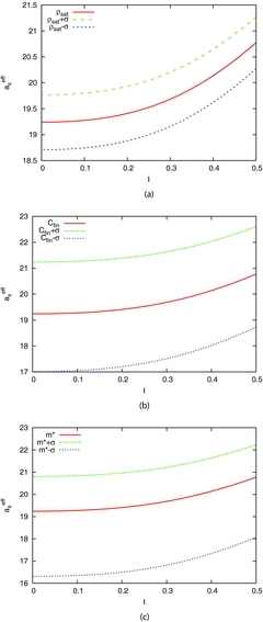
Figure 3. Effect of uncertainty in empirical parameters on the variation of effective surface energy coefficient with asymmetry I. (a) Uncertainty in saturation density. (b) Uncertainty in finite size parameter. (c) Uncertainty in effective mass.

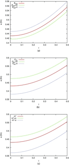
Figure 4. Effect of uncertainty in empirical parameters on the variation of diffuseness parameter with asymmetry I. (a) Uncertainty in incompressibility. (b) Uncertainty in finite size parameter. (c) Uncertainty in effective mass.
3.2. Estimate of finite size parameter using nuclear masses
The estimation of C fin in the previous section relies on the uniqueness of the definition of the surface energy. Unfortunately, the surface energy is not a direct experimental observable and the distinction between bulk and surface requires some modelling. Therefore, we cannot be sure that the functional obtained leads to a reasonable estimation of the nuclear masses. In an alternative approach, we constrain C fin using a fit to experimental nuclear masses. For a range of nuclear masses A, we plot the difference in energy per particle, calculated using ETF model (including Coulomb contribution) and experimental values from AME2012 mass table (Audi et al. Reference Audi, Wang, Wapstra, Kondev, MacCormick, Xu and Pfeiffer2011; Wang et al. Reference Wang, Audi, Wapstra, Kondev, MacCormick, Xu and Pfeiffer2012).
To adjust the value of C fin, we calculate the value of
 $$\begin{equation*}
\chi ^2 = \frac{1}{N} \sum _{i=1}^N \left(\frac{E^i_{\text{th}}-E^i_{\text{exp}}}{E^i_{\text{exp}}}\right)^2
\end{equation*}$$
$$\begin{equation*}
\chi ^2 = \frac{1}{N} \sum _{i=1}^N \left(\frac{E^i_{\text{th}}-E^i_{\text{exp}}}{E^i_{\text{exp}}}\right)^2
\end{equation*}$$
for different (ρsat, C fin, C so). The value corresponding to the minimum of χ2 at ρsat = 0.154fm−3 is found to be C fin = 61 corresponding to C so = 40, while that corresponding to C so = 0 is C fin = 59. The corresponding plot for the residuals is displayed in Figure 5 for the two choices of finite size parameters. It is evident from the figure that the effect of changing the value of C so on the minimum of the energy is negligible.

Figure 5. Difference between theoretical and experimental values of energy of symmetric nuclei per particle, for the two choices of finite size parameters in Section 3.2.
In order to study the sensitivity of the energy per particle to the uncertainty in the empirical parameters, the effect of variations of the isoscalar empirical parameters (ρsat, E sat, K sat) within error bars on the energy residuals is displayed in Figure 6. It is evident from the figure that apart from the effective mass, C fin has the largest effect on the energy residuals.

Figure 6. Sensitivity of the difference between theoretical and experimental values of energy of symmetric nuclei per particle, to the uncertainty in isoscalar empirical parameters.
3.3. Asymmetric nuclei
The uncertainty in isovector empirical parameters only affects the energy residuals at large asymmetry I (Figure 7).

Figure 7. Sensitivity of the difference between theoretical and experimental values of energy per particle vs asymmetry parameter I for Z = 50, to the uncertainty in isovector empirical parameters.
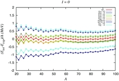
To study the effect of the finite size parameter on the energy per particle of asymmetric nuclei, in Figure 8, we display the residuals for Z = 20, 28, 50, 82. We find that the residuals are close to zero even for finite asymmetry. Therefore, only fixing C fin leads to a good reproduction of energies even for asymmetric nuclei. This justifies the use of a single finite size parameter C fin for symmetric as well as asymmetric nuclei.

Figure 8. Difference between theoretical and experimental values of energy of nuclei per particle vs asymmetry parameter I for different Z values (20, 28, 50, 82).
The uncertainty in the finite size parameter C fin is estimated by varying C fin such that the residuals (E th − E exp)/A lie within ± 0.5 MeV, which leads to an approximate error estimate of 13 MeV (see Figure 9). One may vary C fin within this uncertainty range to reproduce with increasing precision the energy residuals. However, as our simplified model does not include contributions from shell effects and deformations, we cannot aim for precision less than 0.1 MeV in the energy per particle. We have checked that asking for a precision within 0.1 MeV instead than 0.5 MeV does not change the results presented below.

Figure 9. Difference between calculated and experimentally measured energy per particle of nuclei as a function of A for Z = 50.
4 TESTING THE MODEL AGAINST NUCLEAR OBSERVABLES: STUDY OF RMS CHARGE NUCLEI
Matter at subsaturation densities, such as that in the NS crust, is accessible to terrestrial nuclear experiments. In order to test the model developed in Section 3, we calculate the root-mean-square (rms) radii of protons 〈r p 〉 and neutrons 〈r n 〉. To compare with the observations, one must calculate the charge radius that is related to the proton radius, using the following relation:
 $$\begin{equation*}
\langle r^2 \rangle _{ch}^{1/2} = \left[ \langle r^2 \rangle _p + S_p^2 \right]^{1/2},
\end{equation*}$$
$$\begin{equation*}
\langle r^2 \rangle _{ch}^{1/2} = \left[ \langle r^2 \rangle _p + S_p^2 \right]^{1/2},
\end{equation*}$$
where S p = 0.8 fm is the rms radius of charge distribution of protons (Buchinger et al. Reference Buchinger, Crawford, Dutta, Pearson and Tondeur1994; Patyk et al. Reference Patyk, Baran, Berger, Dechargé, Ring and Sobiczewski1999).
For the previously estimated uncertainty in C fin, we plot the charge radii for Z = 50 and compare them with experimental data (Angeli & Marinova Reference Angeli and Marinova2013) in Figure 10. It is found that the experimental values of charge radii span the uncertainty band in C fin: it overestimates the values at C fin + σ, while it underestimates the values at C fin − σ.

Figure 10. The rms charge radii vs asymmetry I for Z = 50, calculated theoretically within uncertainty range of the finite size parameter, compared with experimental values.
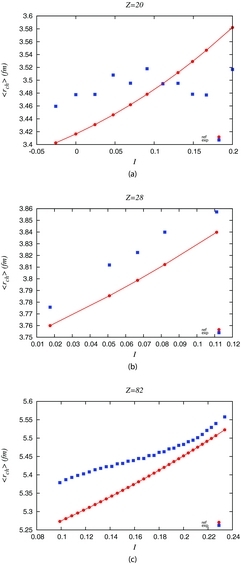
Similarly, the rms charge radii calculated using the above model for Z = 20, 28 and 82 are also compared with experimental data in Figure 11.

Figure 11. Comparison of calculated and experimental rms charge radii with different asymmetry I for different Z nuclei. (a) Z = 20. (b) Z = 28. (c) Z = 82.
5 SUMMARY AND OUTLOOK
In this work, we developed an empirical ‘unified’ formalism to describe both homogeneous nuclear matter in the NS core as well as asymmetric nuclei in the crust. We used DFT in the ETF approximation to construct an energy functional for homogeneous nuclear matter and clusterised matter. In homogeneous nuclear matter, the coefficients of the energy functional are directly related to experimentally determined empirical parameters. We showed in this study that for non-homogeneous matter, a single effective parameter is sufficient (C fin) to reproduce the experimental measurements of nuclear masses in symmetric and asymmetric nuclei. We also tested our scheme against measurements of nuclear charge radii.
In an associated work (Chatterjee et al. Reference Chatterjee, Gulminelli, Raduta and Margueron2017), we employ this model in order to perform a detailed systematic investigation of the influence of uncertainties in empirical parameters scanning the entire available parameter space, subject to the constraint of reproduction of nuclear mass measurements. With the optimised model, we then predict nuclear observables such as charge radii, neutron skin, and explore the correlations among the different empirical parameters as well as the nuclear observables.
ACKNOWLEDGEMENTS
The authors are grateful to Jerome Margueron and Adriana R. Raduta for in-depth discussions and insightful suggestions. DC acknowledges support from CNRS and LPC/ENSICAEN.