


INTRODUCTION
Here we present a novel approach to developing a radiocarbon-based chronology for a set of sediment cores collected in a location where radiocarbon dating has been challenging. The sediment cores analyzed for this project include eight terminal Pleistocene and Holocene cores with correlated stratigraphies (30 cal ka to modern) collected from the western Lake Bonneville basin of western Utah (Figure 1; hereafter LBB; core site descriptions are presented as supplementary information [SI]). The period studied encompasses the rise and fall of late Pleistocene pluvial Lake Bonneville, which has been extensively studied.

Figure 1 Map of core sites showing their locations within the western Lake Bonneville basin of western North America. Lake Bonneville maximum extent is shown with blue shading in panel B. 1. WB-19; 2. ORB-HS-14; 3. DS-17; 4. NRS-14; 5. RSP-15; 6. RSP-18; 7. BCS-15; 8. LCFSN-16. FS NWR = Fish Springs National Wildlife Refuge.
Lake Bonneville was the largest Pleistocene lake in the Great Basin of western North America (Gilbert Reference Gilbert1890; Morrison Reference Morrison1991). The understanding of the chronology of Lake Bonneville has evolved over many years with input from many people (for example, Broecker and Kaufman Reference Broecker and Kaufman1965; Morrison and Frye Reference Morrison and Frye1965; Scott et al. Reference Scott, McCoy, Shroba and Rubin1983; Currey and Oviatt Reference Currey, Oviatt, Kay and Diaz1985; Oviatt et al. Reference Oviatt, Currey and Sack1992; Godsey et al. Reference Godsey, Currey and Chan2005; Oviatt Reference Oviatt2015). The overall accuracy of the chronology is good, but improvements in the chronology are underway (Laabs et al. Reference Laabs, Oviatt and Jewell2019; Oviatt Reference Oviatt2020) and future refinements are certain to be published.
As summarized by Oviatt (Reference Oviatt2015) Lake Bonneville began rising in its hydrographically closed basin from elevations similar to those of modern Great Salt Lake (close to 1280 masl) about 30 cal ka (Figure 2). The lake reached its highest elevation, roughly 300 m higher than 1300 masl, about 18 cal ka, when it began overflowing to the Columbia River drainage basin via the Snake River. The surface elevation of the lake fell about 125 m in a catastrophic event called the Bonneville flood, caused by rapid entrenchment of an alluvial fan in landslide deposits in southern Idaho. The best available age estimates for the Bonneville flood place it within “several hundred years” of 18,000 cal BP (Oviatt Reference Oviatt2015). The flood halted when downcutting at the Red Rocks Pass overflow point reached bedrock. The lake then continued to overflow non-catastrophically as an open-basin lake for an as-yet unestimated amount of time possibly as long as 3000 years. After the lake ceased overflowing and once again became a closed-basin lake it fell in elevation until ∼13 cal ka when it reached Great Salt Lake levels. The Bonneville lake cycle is approximately correlative with global marine oxygen isotope stage 2.
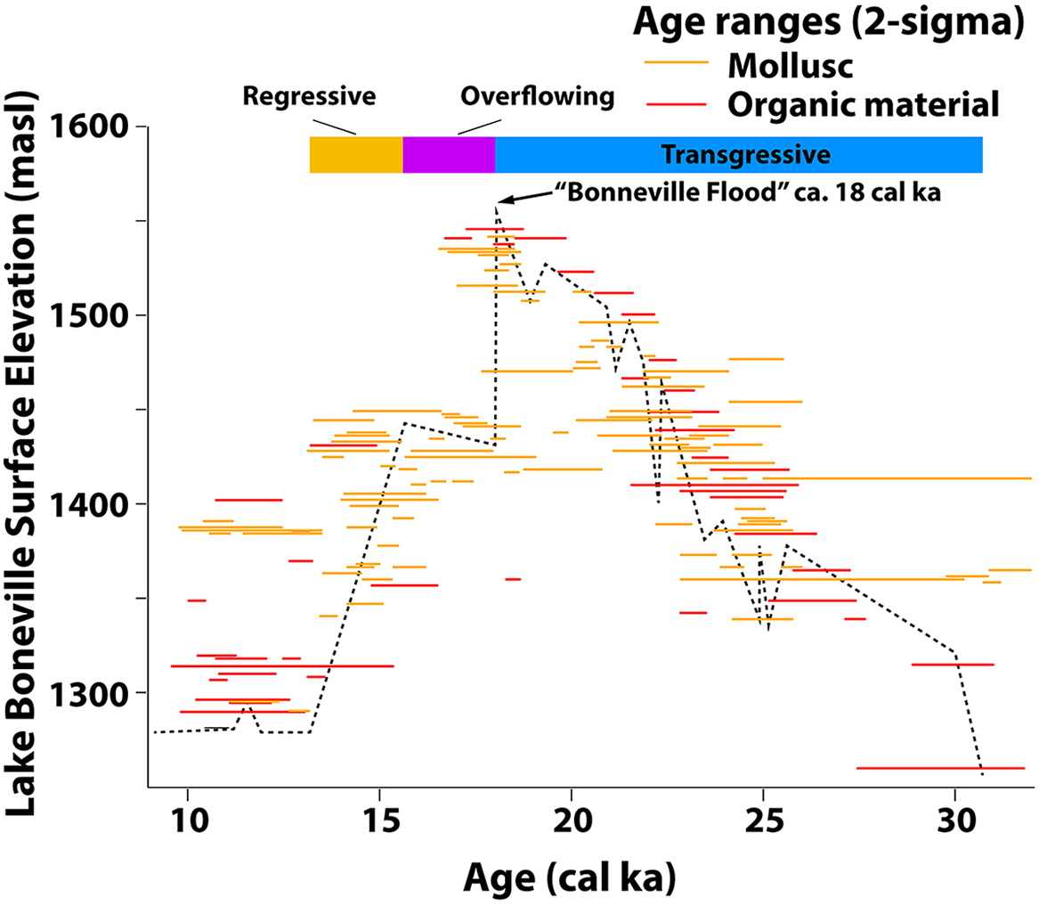
Figure 2 Hydrograph of Lake Bonneville surface elevations, redrawn from Oviatt (Reference Oviatt2015).
Most ages that make up the Lake Bonneville chronology are radiocarbon ages of samples collected by numerous researchers since the 1950s from outcrops in shorezone positions. An advantage of using shorezone chronologies is that the size of the lake at various times in its history can be determined, and this reveals explicit information about paleoclimate. However, some excellent ages are derived from sediments from cores of lake sediment in offshore positions, and it would be useful to be able to confidently link the offshore sedimentary record with the shoreline record. This would, for example, allow detailed correlation of well-dated shorelines with sedimentary paleoenvironmental records. This paper is part of a larger study examining the west desert region of the LBB to understand the paleoenvironments and resources available to early people, as a tool for archaeological predictive modeling and field research. But in order to correlate the multiple cores collected for this larger study with the spatially and temporally heterogeneous archaeological record, a robust, accurate and well-documented chronology must be constructed. This paper develops that chronology, which will serve the current research and is also valuable to ongoing research including the correlation of shorezone/offshore records.
Developing a uniform chronology for our suite of sediment cores emerged as a goal largely because establishing chronological control for individual cores in this project has been challenging. In order to control as many variables as possible in our radiocarbon dating, we have dated almost exclusively pollen samples which have been concentrated by chemical digestion (Table 1). Pollen is produced in terrestrial settings and in ideal conditions should have a reduced susceptibility to radiocarbon contamination from a variety of sources in lake basin settings. Furthermore, pollen is an excellent material for radiocarbon analysis because ultimately, it is also one of the main paleoenvironmental proxies used in paleoecological reconstruction; if understanding variation in pollen abundances over time is the goal of applying a radiocarbon analysis to a sediment core, it would seem that the pollen itself would be an ideal material to submit for radiocarbon analysis. This approach has provided excellent results for previous studies (e.g., Carter et al. Reference Carter, Brunelle, Power, DeRose, Bekker, Hart, Brewer, Spangler, Robinson, Abbott and Maezumi2021; Hart et al. Reference Hart, Brenner-Coltrain, Boomgarden, Brunelle, Coats, Metcalfe and Lewis2021).
Table 1. Radiocarbon ages used in age-depth model.

* Unless otherwise noted, all ages were derived from concentrated pollen samples.
† Calibration used the Intcal20 calibration curve (Reimer et al. 2020).
a Modern surface age of AD 2018 (–68 ± 20 BP) applied to depth zero.
b Bulk sediment ages from Wishbone Stratum are from from Duke et al. (Reference Duke, Rice, Young and Byerly2018).
c BCS15 395–396 age was generated from sculpin (Cottidae: Cottus) bones found in situ in the core.
But even with dating mostly pollen samples, all of our cores show age reversals, and core-specific age-depth models have resulted in sections of different cores which appear stratigraphically identical having estimated ages that are thousands of years apart. This could be a result of a variable hardwater radiocarbon reservoir effect in Lake Bonneville. The ability of old water to deplete hydrologic systems of radioactive 14C has been known for decades (e.g., Tamers Reference Tamers1967), and has previously discussed with respect to Lake Bonneville sediments by Rey et al. (Reference Rey, Mayo, Tingey and Nelson2016). Variation in groundwater discharge and atmospheric mixing has been demonstrated to have affected the radiocarbon budget of lake Bonneville over time and within different sub-basins of the lake (Oviatt Reference Oviatt2015). Lake Bonneville’s surface level fluctuated dramatically over the course of the lake’s history, and during each fluctuation, groundwater discharge rates and transit-times also changed, thus affecting the radiocarbon reservoir of the lake water. While pollen is from terrestrial plants and should not be susceptible to old carbon contamination, algae in a lake might have access to old carbon from groundwater inputs to the lake, and algae and algal spores are not destroyed by the chemical digestion process used here to concentrate pollen. It is therefore possible that the inclusion of those spores and/or non-pollen organic matter which survived the pollen-preparation procedures may cause some of the observed reversals in the reported ages.
Standard practice in paleoecology when confronting sets of radiocarbon ages with reversals is to eliminate those ages which seem to be suspect based on some independent line of evidence, with the assumption that stratigraphic integrity and the law of superposition supersedes the uncertainty associated with radiometric dating. For example, if a radiocarbon age of infinite age appears in a sequence of otherwise stratigraphically consistent Holocene radiocarbon ages, most researchers would reject the infinite age as contaminated with old carbon. Similarly, ages generated from different materials are often accepted or rejected based on their perceived fit into known stratigraphies or existing age models. In dating Lake Bonneville shoreline deposits, Oviatt (Reference Oviatt2015) for example rejected ages from carbonate materials which were older than wood or charcoal ages from similar stratigraphic positions, likely because of radiocarbon reservoir effects. Since we almost exclusively dated concentrated pollen samples, in most cases there was nothing about any particular age other than the age itself to give us reason to accept or reject it. However, a few stratigraphic markers allowed us to evaluate certain ages and anchor the chronology in time. For example, we have identified Mount Mazama volcanic ash in one of the cores (RSP-15B, see SI for site description) at a depth of 99 cm. The eruption of Mount Mazama dates to 6845 ± 50 BP with a median calibrated age of 7673 cal BP (Bacon Reference Bacon1983). But radiocarbon analysis of a sample from 110 cm in the same core returned an age of 4804 ± 26 BP (median 5518 cal BP). However, subsequent radiocarbon re-analysis of a second sample from 110 cm depth in the core returned an age of 9011 ± 27 BP (median calibrated age of 10205 cal BP). We discarded the younger age as likely contaminated by younger carbon.
Radiocarbon ages can also be skewed by young carbon in many ways including microbial contamination if the sediments are not stored properly or for too long (Wohlfarth et al. Reference Wohlfarth, Skog, Possnert and Holmquist1998). Sediments can contain modern rootlets, which would result in an erroneously young age. Mahaney and Boyer (Reference Mahaney and Boyer1986) also propose that sediments can be contaminated by bacteria and fungi that occur on roots or rootlets that penetrate the older material. A recent publication also posits that fungal hyphae from tree roots can contaminate a sample with young organic material (Karig et al. Reference Karig, Mayers, Wattenburge and Southon2021). As we mainly cored wetland areas, the possibility of modern rootlet contamination exists.
Fortunately, the cores used in this project show excellent preservation of visible stratigraphy, consistent from core to core, and we have been able to take advantage of multiple ages from different cores using a stratigraphic correlation approach. In addition to using visually identifiable stratigraphy to correlate cores for identical stratigraphic sections, we have used high resolution X-ray fluorescence data to provide index depths for several basin-wide geochemical changes in Lake Bonneville sediments which appear in sections of cores which do not have sufficiently identifiable visual stratigraphy. The XRF data have provided an additional dataset to align cores. Aligning visible stratigraphies along with the XRF data has allowed us to use a novel approach to chronology building, dating several cores at once rather than one at a time, and it has allowed us to make sense of an otherwise problematic radiocarbon age distribution with potentially multiple sources of contamination.
METHODS AND RESULTS
Coring
We used a “vibracore” system (Lanesky et al. Reference Lanesky, Logan, Brown and Hine1979) to collect eight cores from the LBB of western Utah for this analysis. The vibracore system consists of a concrete leveling vibrator powered by a 2.5 horsepower petrol motor. The vibrator assembly is attached via a custom-made clamp to a 20-foot (6.1 m) long aluminum irrigation tube with a 3” (7.62 cm) outside diameter and a .065” (1.65 mm) wall thickness. The end of each tube is sharpened with a bastard file before coring, to ensure root mat/vegetation penetration. For each core, the tube is vibrated with the motor, and driven down by gravity with field crew personnel pulling down until friction or changes in stratigraphy prevent additional downward movement of the core tube. After removal from the ground, the cores are capped and transported whole to the cold storage facility in the Records of Environment and Disturbance laboratory at the University of Utah.
To open the cores, we used a 7” electrical circular saw with a bi-metal blade to split the tube lengthwise, cutting only the tube itself on opposing sides without cutting the core material. We then use a thin gauge steel wire to pass upwards through the core along the cut tube edges, splitting the core in half and allowing it to be opened, preserving visible stratigraphy and providing a clean profile for XRF scanning. To clean the face of each core half prior to photography and XRF-scanning, we use a 3” scraper with distilled, deionized water cleaning between each pass, scraping horizontally across the core. Half of the core is then cut into 1-m sections and stored in airtight tubes in the cold storage facility for archival purposes. The non-archival half is photographed (described below), then cut into 1-m sections for high resolution XRF scanning (described below), and then placed in cold storage.
Photographic Alignment
The approach we report here involved aligning the cores in time using preserved visual stratigraphy where applicable and high-resolution X-ray fluorescence based elemental composition data (below) where visible stratigraphy is not correlatable. The first step in photographic alignment of the cores involved generating high resolution photographs of each core. Photography of the cores immediately follows opening the cores in order to best capture the visible stratigraphy, which can begin to fade as soon as the cores are exposed to air for even as little as an hour. To generate the highest resolution possible and provide a method with the highest replicability and lowest cost, we chose to use a digital SLR camera for our core images rather than a dedicated core scanner. To photograph the cores, we used a Canon EOS 80D digital SLR camera with a Canon 100mm f/2.8L macro lens to photograph 15-cm sections of each core, with at least 4 cm of overlap between each image pair. This resulted in images with resolutions of around 400 pixels per cm of sediment (about 25 microns/pixel).
Several steps and parameters were required to combine the individual photographs into usable core images, minimizing parallax and color errors and preserving size relationships across the cores. First, all cores were photographed using identical laboratory lighting and with identical camera settings (ISO, aperture, shutter speed and white balance). All photographs for each core were also taken with identical focal lengths. To achieve this we used a rolling core holder which held the face of the core at a constant distance from the camera as it passed under the camera, which was mounted to a bench. This resulted in a set of images for each core which could be aligned and stitched in a way which reasonably minimized parallax and color error.
We used the open-source panoramic photography stitching software Hugin (http://hugin.sourceforge.net) to align and stitch the photographs into single images. At least 25 “normal” and four “horizontal line” alignment control points were generated between each image pair. All control points generated for positions in the image outside the focal plane of the face of the core were removed. Stitching for each core image used an equirectangular projection and was executed at the maximum possible resolution for each image. Photographs of the cores before and after the alignment steps described below are provided in Figure 3.

Figure 3 Core photographs before (A) and after (B) vertical alignment. 1: RSP-18; 2: RSP-15; 3: BCS-15; 4: NRS-14; 5: WB-19; 6: LCFSN-16; 7: DS-17; 8: ORB-HS-14. Smaller numbers overlaid on core images correspond to radiocarbon ages presented in Table 1. Panel (C) shows RSP-18 section 238-352, RSP-15 section 257-358, BCS-15 166-333, NRS-14 section 281-377, WB-19 section 158-202, LCFSN-16 section 211-244, DS-17 section 100-149, ORB-HS-14 section 74-115.
While the resulting images preserve visible stratigraphy very well, the method used here of photographing multiple sections of each core and combining the photographs into one image does introduce size and parallax error—a 1-cm object at the center of an image may not be the same number of pixels as 1 cm at the edge of the image. This error is added many times as the photographs are stitched together as the software has no algorithm to re-size different portions of each photograph according to a pre-defined scale or warp factor. To overcome this limitation, we cut the complete single-image core photographs up into sections of approximately the size of each original photograph, and manually reassembled the image in Adobe Illustrator. We stretched each photograph section to a predefined scale, such that the horizontal size of each centimeter in the final image (we assembled the images horizontally so that left was top and right was bottom) was constant for each centimeter in the image. This process worked well, and none of the final images had horizontal error more than 1 mm at any position in the photograph. This met our goal for horizontal precision because our XRF core scanner scans at 2-mm resolution; to make our XRF data comparable to our photographs we needed a photographic horizontal precision of at least the resolution of the XRF scans, and this was achieved.
After photographing all eight of the cores used in this analysis, several patterns were clear. First, while none of the cores appeared to line up with any of the other cores perfectly (with the exception of the RSP-15 and RSP-18 cores, which were collected only about 2 m apart), sections of each core did appear to visually match sections of other cores. One common feature of the set of cores was that they do appear to more or less match up in broad trends over time despite the 50 km diameter of the study area. The lowest section of each core contains sections of finely laminated marl, which has been identified in several outcrops and cores in early Lake Bonneville deposits across the LBB (e.g., Oviatt et al. Reference Oviatt, Currey and Miller1990; Rey et al. Reference Rey, Mayo, Tingey and Nelson2016). The finely laminated marl transitions to thicker laminations of massive marl, which then gives way to a massive marl section in each core. Finally, in some of the cores, particularly those nearer to permanent water sources (the active spring cores), a thick organic section occurs above the massive marl (Figure 3).
As a baseline with which to align all of the cores and to assign uniform depth values to identical stratigraphic events found in multiple cores, we used the longest and best visually preserved core we have collected to date, the RSP-18 core. We used a cut and stretch/compress method in Adobe Photoshop, stretching or compressing smaller vertical sections of the photograph of each core so that a visual alignment with core RSP18 was obtained. This process resulted in core images with very closely matching stratigraphy across the laminated marl sections (Figure 3). For the massive marl sections, there was insufficient stratigraphic variation to allow any meaningful attempt at stratigraphic correlation. For these sections we used the XRF-based elemental abundance data for stratigraphic alignment (described below).
During our alignment of the core images, we identified another notable feature of the different cores when compared with one another. Different sections of some cores which have matching stratigraphy are of quite different vertical thicknesses. The 100–115 cm section of core ORB-HS-14 for example aligns with the 292–346 cm section of core RSP-18 and with the 210–325 cm section of core BCS-15 (Figure 3). Thus 15 cm in one core spans the same time period as a 54 cm section of another core, and a 115 cm section of a third core. We interpret the differing thicknesses of the matching stratigraphic sections of the cores as indicating variations in sedimentation rates across the LBB. Variability in marl sedimentation rates and connections between sedimentation and geomorphology during the Bonneville cycle has been documented (Oviatt Reference Oviatt2018), and one of the primary factors determining sedimentation rate across the basin is distance from shore (Table 1). The ORB-HS-14 core site for example is about 15 km from the nearest Lake Bonneville shoreline. The site likely had very little alluvial or colluvial sediment input during Lake Bonneville times and therefore very slow deposition rates. The BCS-15 site however sits at the toe of the Fish Springs range, within 1 km of several Lake Bonneville shorelines which allowed much more rapid sediment deposition at that site during a wide range of lake levels.
XRF-Based Alignment
X-ray fluorescence (XRF) is a relatively quick and nondestructive methodology that provides high-resolution elemental analysis, making it an ideal application for paleoecological studies of sediment cores (Croudace and Rothwell Reference Croudace and Rothwell2015). We used XRF-derived elemental concentrations data for this study to correlate the sections of our sediment cores which do not have visibly preserved stratigraphy. Specifically, the massive marl sections of the cores analyzed in this paper do not have sufficiently visible stratigraphy for photographic alignment. These cores do however record lake basin-wide changes in elemental concentrations of sediments deposited during Lake Bonneville times. For the sections of the cores with no correlatable visual stratigraphy, we used a stratigraphic correlation approach similar to the photographic cut and stretch method described above, taking advantage of high resolution XRF-based elemental analysis we had originally collected to evaluate basin-wide geochemical changes in sediments associated with variations in Lake Bonneville’s hydrographic history.
We used a Rhodium-anode Bruker Tracer IIISD series handheld pXRF (T3S2756 and T3S2776) with a silicon-drift detector with a resolution of 140 eV at full-width height maximum for manganese (Mn) K-alpha mounted on a Dewitt Systems MCS-800 Mobile Core System. We scanned each sediment core at 2-mm increments to produce a continuous high-resolution elemental record. Measurements were taken for 60 s using two settings: (1) 15kV, 10mA, and helium gas, and (2) 40kV, 30mA, and yellow filter (25μm Ti/300μm Al) without helium.
Data were collected as raw photon counts and were divided by the instrument live time, generating values referred to as “photon intensities” with a unit of counts per second (c/s). The photon intensities were calibrated into elemental concentrations using the mudrock reference set and methods discussed by Rowe et al. (Reference Rowe, Hughes and Robinson2012) using S1PXRF and S1Cal Process (V. 2.2.32). XRF spectra were normalized to Compton. A Compton energy range of 2.8–3.2 KeV was used for light elements captured the first setting (15kV, 10mA, helium gas), and an energy range of 18.5–19.5 KeV for heavier elements captured in the second setting (40kV, 30mA, yellow filter).
While handheld XRF units are not typically used for this level of detail or range of elements, it is feasible if measurement parameters are carefully tuned with XRF physics. Typically, XRF data analysis used in previous sediment core studies have used photon intensities or Bayesian deconvolution methods to extract net photon counts rather than calibrated concentration data (Elam et al. Reference Elam, Scruggs, Eggert and Nicolosi2010).
In our data collection process, the flow of helium removes the attenuation of air, which allows the measurement of Na and Mg down to 0.7% (Rowe et al. Reference Rowe, Hughes and Robinson2012). The use of a heavily attenuating filter, by contrast, strongly reduces the effects of bremsstrahlung radiation and allows for low-level detection of trace elements (Brent et al. Reference Brent, Wines, Luther, Irving, Collins and Drake2017).
To take advantage of all the resulting XRF data available for each core simultaneously, we used a principal components analysis (PCA) approach, executing a separate PCA for each core’s complete dataset in the statistical programing software R. PCA results for each sediment core are presented in the supplementary information file. Our PCA analyses showed that in each core, the first component of variance explained about 60% of the variation in the scores (Figures S1-S5). Furthermore, at the coarsest level of resolution, the largest source of variation appears to have been differences in hydrologic context between late Pleistocene lacustrine deposition and Holocene terrestrial aquatic (wetland) depositional environments. The uppermost portions of the cores, which had thick organic post-Bonneville (Holocene) mud sections have uniformly low first principal component (PC) scores, whereas the massive and laminated marl (Pleistocene lake deposits) had much more variable, and consistently higher, first PC scores. Our interpretation of this pattern is that the largest amount of variation in these data concern the difference between lacustrine and terrestrial aquatic depositional environments. With this observation in hand, we used the first PC for each dataset, plotted as a time series by depth, to align the sections of the cores which we were unable to align using visual stratigraphy. First principal component scores for each core before visual and XRF-based alignment are shown plotted by depth in Panel A of Figure 4. The same data are plotted by age after alignment are presented in Panel B of Figure 4.

Figure 4 First principal component scores for each core’s XRF dataset as time series, plotted by depth before (Panel A) and after (Panel B) XRF-based and photographic alignment. Labels A–D mark study area-wide hydrographic events used for vertical alignment of the massive marl sections of the cores. Label E marks the top of the visually aligned section of cores RSP-18. WB-19, LCFSN-16, and DS-17. Label F marks the top of the visually aligned section of core BCS-15.
After plotting the time series of the first PC for each core, we identified four positions in each core which appear to mark basin-wide XRF events in the non-laminated sections of the cores. These positions are labeled in Figure 4 as A–D. Position A marks what appears to be the most significant change in the record, a change from variable first PC scores below to uniformly low first PC scores above. Position B marks a diagnostic global spike in the first PC which is present in all of the cores. Positions C and D mark less extreme but identifiable spikes in the first PC score for each core except BCS-15. Data are missing from that core where C and D would be because the core’s surface after cutting was too rough to allow our XRF scanner to get close enough to the surface of the core (within 0.2 cm) to return reliable scan results. Position E marks the top of the laminated marl sections of each of the cores except BCS-15. Below this point, visual alignment was sufficient. Position F marks the top of the laminated marl section of core BCS-15, below which visual stratigraphy was used for alignment.
Unaligned Section
For the section above the visually matching and XRF-matched sediments, we have no independent dataset with which to correlate the cores. The only exception to this is the RSP18 and RSP15 cores, which are visually nearly identical (Figure 3), having been collected from sites only 2 m apart. Because of this we used only the ages from RSP15 and RSP18 for the 0–114 cm section of the age-depth model, and all available ages from 114 to 510 cm. Functionally, this means that the composite age-depth model can be applied to the entirety of RSP15 and RSP18 but only to the visually and XRF-matched sections of the remaining cores. The break point between the aligned sections of the cores (below 114 cm) and the unaligned sections (above 114 cm) appears to correspond to the final regression of Lake Bonneville, about 13 cal ka BP. Sediments below this point were deposited in generally deep-water conditions, while sediments above this point in most cores were deposited in shallow wetland conditions. For subsequent analyses of these cores, the composite model can be applied to the lacustrine sections of the cores but each core will need an independently generated age-depth model for the sections post-dating 13 cal ka.
Radiocarbon Ages
We used a total of 37 radiocarbon ages to construct the age-depth model presented here. These ages are presented in Table 1. Thirty-one ages were generated from samples collected from four of the sediment cores. In addition to the radiocarbon ages derived directly from the four cores, we assigned ages of 6845 ± 50 BP (7673 cal BP median age) to levels in cores RSP15 and RSP18 from which we identified shards of Mazama ash, a well-known and well dated volcanic tephra found in sites across western North America (Bacon Reference Bacon1983). These shards were identified via electron microprobe analysis. Three additional radiocarbon ages were assigned to a black mat layer found in core WB19. This core was collected near an archaeological site called the “Wishbone site,” which was excavated and reported by Duke et al. (Reference Duke, Rice, Young and Byerly2018, Reference Duke, Wohlgemuth, Adams, Armstrong-Ingram, Rice and Young2021). During archaeological excavation at the site a deep probe was dug, the profile of which revealed the same terminal Pleistocene black mat. Three radiocarbon ages were generated from bulk organic samples from the black mat at the Wishbone site (Table 1). We applied the three ages from that stratigraphic unit to the WB19 core at the vertical position the black mat appears in that core. Finally, because we encountered modern vegetation and algae growing in active wetland sediments at the surface of both Redden Springs cores, we applied a modern radiocarbon age of –68 ± 20 BP (AD 2018, the year core RSP18 was collected) to the surface depth of zero. In an earlier iteration of the age-depth model, failure to anchor the surface to a modern age resulted in a predicted age of surface sediments of –500 cal BP (AD 2550) which we felt was not appropriate and skewed the chronology for the younger part of the core. The three cores for which we did not generate radiocarbon ages were included in this analysis to increase our confidence in the stratigraphic correlations we used, as well as to demonstrate the applicability of the method in applying chronological control to otherwise undated sediments.
Of the 31 radiocarbon ages derived from materials sampled from the cores, all but one were derived from concentrated pollen samples. Pollen samples were treated by standard chemical digestion similar to the method described by Faegri et al (Reference Faegri, Kaland and Krzywinski1989). But in order to avoid carbon contamination from acetic acid during the acetolysis step, we instead used a 2-minute treatment with Schulze’s reagent (8 mL nitric acid + 0.8 g potassium chlorate per cc of sample). Samples were checked using light microscopy to verify the presence of pollen, but no attempt at quantification or further concentration was made. The only non-pollen derived radiocarbon age from the cores was an age derived from several sculpin bones (Cottidae: Cottus sp.) identified in core BCS15 at a depth of 395 cm (Table 1).
Bacon
To generate our age-depth model we used the age-depth modeling software Bacon in the “rbacon” package for R (Blaauw and Christen Reference Blaauw and Christen2011). This age-depth modeling approach uses a Bayesian statistical approach including Markov Chain Monte Carlo (MCMC) iterations. This approach allows us to use the full suite of ages across cores to extract the most parsimonious sedimentation scenario. In executing Bacon, we used the default arguments, with ages interpolated to every 0.1 cm and a maximum depth of 510 cm (the bottom of the RSP18 core). Ages for the lowest 50 cm of the age-depth model (below the lowest RSP15 ages at 471–472 cm, which corresponds to 450 cm in RSP18) are therefore extrapolated beyond the actual radiocarbon ages used in the model.
DISCUSSION AND CONCLUSIONS
The age-depth model generated for this project and the calibrated age distributions for each radiocarbon age are presented in Figure 5. The figure shows the probability distribution of each calibrated age, the median calibrated age predicted for each depth in the model, and a 95% confidence envelope for the age-depth model. The probability distribution of each age is labeled with a number corresponding to Table 1 for the purposes of identifying the core from which each age was derived.

Figure 5 Age-depth model created using radiocarbon ages from eight Lake Bonneville Basin sediment cores after aligning the cores using visual stratigraphy and PCA analysis of XRF-based elemental concentrations. Numbers associated with calibration distributions refer to radiocarbon ages numbered in Table 1.
Radiocarbon dating of sediments in the LBB has been challenging given an apparent multitude of opportunities for the sediments to be contaminated with either old or young carbon, or both. The goal of this project was to develop a method of creating a relatively robust composite age model using all the data available to us, with radiocarbon ages from a variety of sites. This composite age model will be used to reconstruct the paleoenvironments of each site, and also to serve as a starting point for further efforts to refine the existing Lake Bonneville hydrograph. One aspect of this model which is troubling, but which also illustrates the necessity of having a single uniform chronology to apply to each these cores, is the distribution of radiocarbon ages relative to the age-depth model itself. As Figure 5 shows, 15 of the calibrated ages from these sediment cores fall outside the confidence envelope of the age-depth model. This is especially problematic for the ages between about 200 and 400 cm. Furthermore, there is no real link between the core from which each age was derived, and whether that age falls above, below, or within the confidence envelope. That is to say, there is no way of guessing which age is more or less suspect based on which core it came from, and so without some additional information, there is no independent reason to include to exclude any particular age in efforts to refine the model. This has resulted in fairly wide confidence intervals for the age model. As can be seen in Figure 5, the confidence envelope for the age-depth model varies considerably over the model from a hundred years or so, to up to 2000 years between 16 and 20 cal ka. For that reason, the present age model is not likely to be particularly useful in refining the timing of specific events such as the Lake Bonneville highstand and the Bonneville Flood without further revision. But this model will serve as a starting point for refining these events as this model is itself refined in the future. One beneficial aspect of the approach detailed here in this regard is that even though the ages for particular parts of the age model may be less refined at this point than they will hopefully be in the future, because we have started by aligning the cores stratigraphically, improvements to the chronology will simultaneously improve our interpretations of multiple different records.
Despite the challenge of the broad scatter of ages, the age-depth model we generated from this set of radiocarbon ages has allowed us to start making sense out of an otherwise troubling set of ages. Taken altogether, this model has produced a chronology that is consistent, reflects likely basin-wide lake level events, and lines up similar depositional events across the suite of cores in time. A coarse comparison to the published chronology for major hydrographic changes helps illustrate this point. Oviatt’s (Reference Oviatt2015) summary of Lake Bonneville’s hydrographic sequence remains the most up to date hydrographic history of the lake, using hundreds of radiocarbon ages from a variety of materials and stratigraphic settings (Figure 2). The broad outline indicates the waters of lake Bonneville began rising around 30.5 cal ka, the lake dropped as a result of the “Bonneville Flood” at around 18 cal ka, and the lake began its final regression from the Provo shoreline some time after 16.5 cal ka. By approximately 13 cal ka, the lake had dropped to a level at or near the modern Great Salt Lake.
Utilizing radiocarbon ages from a suite of cores from different locations around the western portion of the LBB has allowed us to create a relatively robust chronology which can now be used in the analysis and reporting of each of these cores. A Bayesian approach to age modeling allowed the most parsimonious depth-age relationship to be revealed. Using core photographs and XRF analyses for stratigraphic correlation further strengthened the reliability of the final, “master” chronology. This chronology can now be utilized in future analyses to contribute to our understanding of the timing and paleoclimatic significance of changes in Lake Bonneville’s geochemistry and surface elevations. Analyses of cores collected in the future with stratigraphic sections matching sections of these cores will also benefit from being able to use the age-depth model generated here. The chronology developed here will almost certainly be refined in the future as well, taking advantage of radiocarbon ages not yet generated for correlatable cores and sedimentary exposures in future projects.
Finally, while the present study utilized photography, XRF-based elemental data and volcanic tephra identification to identify unique stratigraphic events in multiple sediment cores, the method used here could be applied using any other kind of stratigraphic dataset as well. Suitable datasets could include geochemical analyses such as magnetic susceptibility or loss-on-ignition-based carbonate and total organic carbon. Stratigraphic paleoenvironmental datasets could also be applied in this way with data such as pollen abundance, diatoms, foraminifera, macroscopic charcoal, or any other kind of dataset where unique basin-wide, or even global regional stratigraphic events can be identified.
SUPPLEMENTARY MATERIAL
For supplementary material accompanying this paper visit https://doi.org/10.1017/RDC.2022.3
DATA AVAILABILITY STATEMENT
Data and images used in this study are available upon request via email from the corresponding author.
ACKNOWLEDGMENTS
This paper was improved thanks to very thoughtful reviews provided by Jeff Pigati and one anonymous reviewer. Any errors and weaknesses which remain are solely the responsibility of the authors. This project was funded by the United States Army Dugway Proving Ground Public Works Environmental Programs.


 Open access