


1. Introduction
The Hamiltonian structure of the water-wave problem found by Vladimir Zakharov allows a compact description of dynamics of weakly nonlinear wave fields via a single integro-differential equation; see e.g. Zakharov (Reference Zakharov1968) and also Krasitskii (Reference Krasitskii1994).
To cubic order in surface steepness, the amplitude evolution is governed by the Zakharov equation:
 \begin{equation} \mathrm{i}\,\frac{\mathrm{d} b_1}{\mathrm{d} t} = \omega_1 b_1 + \int{T_{1,2}^{3,4} b_2^* b_3 b_4 \delta_{1,2}^{3,4} \,\mathrm{d}\boldsymbol{k}_{2,3,4}}, \end{equation}
where  $b_{i}=b(\boldsymbol {k}_i,t)$ are complex amplitudes related to the physical variables, characterising the free surface elevation and velocity potential on the surface, through a number of canonical transformations; see Appendix A. Also, $\omega _1^2=\mathrm {g} k_1 \tau _1$, with $k_1=\left \lvert \boldsymbol {k}_1 \right \rvert$ the modulus of the two-dimensional (2-D) wave vector $\boldsymbol {k}_1\in \mathbb {R}^2$, and $\tau _1=\tanh {( k_1 h)}$. Notation is made compact by using subscripts and superscripts: the symbol $\delta$ is the Dirac-delta written in compact notation, i.e. $\delta _{1,2}^{3,4}=\delta {(\boldsymbol {k}_1+\boldsymbol {k}_2-\boldsymbol {k}_3-\boldsymbol {k}_4)}$, $T_{1,2}^{3,4}=T(\boldsymbol {k}_1,\boldsymbol {k}_2,\boldsymbol {k}_3,\boldsymbol {k}_4)$ is the kernel describing the interaction among four waves, and the integration symbol stands for a triple $\mathbb {R}^2$ integration with $\mathrm {d}\boldsymbol {k}_{2,3,4}=\mathrm {d}\boldsymbol {k}_{2}\,\mathrm {d}\boldsymbol {k}_{3}\,\mathrm {d}\boldsymbol {k}_{4}$. The expression for $T_{1,2}^{3,4}$ and all the canonical transformations, summarised in Appendix A, are based on the work by Krasitskii (Reference Krasitskii1994).
Besides being a widely used model for the analysis of fundamental aspects of nonlinear wave propagation, the Zakharov equation (1.1) also provides the basis for the derivation of the kinetic equation (e.g. Zakharov, L'vov & Falkovich Reference Zakharov, L'vov and Falkovich1992; Nazarenko Reference Nazarenko2011); the latter, known as the Hasselmann equation in the water-wave context, is the backbone of the spectral models used e.g. for the ocean wave modelling and forecasting (Komen et al. Reference Komen, Cavaleri, Donelan, Hasselmann, Hasselmann and Janssen1996).
In the deep-water limit, the Zakharov equation raises no concerns and is used widely for modelling of wave dynamics (e.g. Annenkov & Shrira Reference Annenkov and Shrira2001; Janssen Reference Janssen2004). In contrast, the question of whether the Zakharov equation (1.1) is also fully satisfying in water of finite depth (Zakharov Reference Zakharov1999), and hence could be used in practice, has been discussed for decades. The difficulty is that while  $T_{1,2}^{3,4}$ has a well-formed structure, its degenerate forms $T_{1,2}^{1,2}$ and $T_{1,1}^{1,1}$, also known as ‘trivial interaction’ kernels, are not generally defined. The role of the trivial interaction kernels is to account for the Stokes-like frequency shift of the wave harmonic with wave vector $\boldsymbol {k}_1$ caused by the harmonic $\boldsymbol {k}_2$. These interactions are called trivial since they operate only as frequency shifts and do not affect the evolution of the wave amplitudes. The calculation of $T_{1,2}^{1,2}$ is not straightforward and has to be done in the sense of a limit in two dimensions. For example, one has to use the constraint $\boldsymbol {k}_4=\boldsymbol {k}_1+\boldsymbol {k}_2-\boldsymbol {k}_3$ prescribed by the Dirac- $\delta$ in (1.1), and let $\boldsymbol {k}_3\rightarrow \boldsymbol {k}_1$ (e.g. Janssen & Onorato Reference Janssen and Onorato2007). When accounting for finite depth, this limit operation does not return a unique answer (see e.g. Herterich & Hasselmann Reference Herterich and Hasselmann1980), therefore the limit does not exist, i.e. $T_{1,2}^{3,4}$ is singular.
The singularity of the evolution equation kernel originates from the nonlinear canonical transformation that expresses the wave amplitudes in terms of the transformed variable  $b(\boldsymbol {k})$. More specifically, we refer to the part of the transformation that removes the Hamiltonians in the manifold $\boldsymbol {k}_1+\boldsymbol {k}_2=\boldsymbol {k}_3$ and, automatically, in the manifold $\boldsymbol {k}_1=\boldsymbol {k}_2+\boldsymbol {k}_3$, given by (3.13) and (3.14) in Krasitskii (Reference Krasitskii1994), reported here as (A11). The degenerate form of that part of the canonical transformation contributes in setting the surface mean set-up and the wave-induced current. At the four-wave interaction level, the same three-wave interaction kernels enter the canonical transformation as correction to higher moments of the surface elevation and the four-wave interaction kernel of the evolution equation. This is formalised by the four-wave transformation kernel found by Krasitskii (Reference Krasitskii1994) ((3.24) therein), which corresponds to our (A12c). The latter enters the cohomological equation (3.5) by Krasitskii (Reference Krasitskii1994) and thus determines the evolution equation kernel. As a result, the degenerate form of the three-wave kernels are the cause of the non-uniqueness of the trivial interaction kernel. To summarise, the non-uniqueness of the mean set-up of the wave-induced current and of the nonlinear frequency shift have the same origin.
The present work aims to clarify the nature of the singularities in the kernels and thus remove the obstacles to using the Zakharov equation for finite depth. It is motivated by the question: If this ‘theory’ indeed has a singularity, is it legitimate to disregard it and keep only the regular part? This is truly crucial not only for coherence of the theory, but because of all important practical applications, such as ocean-wave modelling in finite water depths. First, we'll try to examine whether the singularities of the kernels manifest themselves as actual singularities of the equations.
To understand the origin of the singular terms, it is convenient to express the kernel  $T_{1,2}^{3,4}$ as
 \begin{equation} T_{1,2}^{3,4} = 2 H_{1,2}^{3,4} + R_{1,2}^{3,4} + S_{1,2}^{3,4} + S_{1,2}^{4,3}, \end{equation}
where  $H_{1,2}^{3,4}$ is a well-defined function governing interactions of two wave pairs, while the last three terms are a result of the canonical integral transformation eliminating all triad interactions, relegating them to the status of second-order ‘bound modes’ (see e.g. (2.17) in Krasitskii Reference Krasitskii1994). The $R$ term is linked to the elimination of the super-harmonics, while the $S$ terms are the result of the removal of the sub-harmonics. These $S$ terms are referred to as ‘singular’ by Stiassnie & Gramstad (Reference Stiassnie and Gramstad2009), since $S$ kernels are not defined on the manifolds $\boldsymbol {k}_3=\boldsymbol {k}_1$ and $\boldsymbol {k}_3=\boldsymbol {k}_2$, i.e. the ‘limits’ $S_{1,1}^{1,1}$ and $S_{1,2}^{2,1}$ do not exist. These manifolds are responsible for the wave-induced current and mean set-up.
At this point, one might wonder whether the removal of the sub-harmonics from the equation of motion makes sense, or if the nearly resonant triad interactions are really important for the dynamics. Herterich & Hasselmann (Reference Herterich and Hasselmann1980), concentrating on the errors associated with an improper treatment of the singularity of the sole self-interaction kernel, suggested removing the uncertainty just by averaging over the limit approaching direction, and then forcing this average to be zero. Zakharov & Kuznetsov (Reference Zakharov and Kuznetsov1997), however, observe that in systems with such dispersion laws, where  $\omega$ is becoming linear as $k\downarrow 0$, the low-frequency motion has to be described by a separate equation.
The issue related to the mean flow, wave-induced or not, is pervading the various approaches to the problem. For example, Madsen & Fuhrman (Reference Madsen and Fuhrman2006, Reference Madsen and Fuhrman2012), by means of a classical perturbation method and admitting a stationary ambient current, found a well-defined Stokes-like frequency shift, but the transfer functions turn out to be unbounded on the resonant manifold. Janssen & Onorato (Reference Janssen and Onorato2007), under assumptions of narrow band and one-dimensional (1-D) wave propagation, found a well-defined self-resonant kernel  $T_{1,1}^{1,1}$, and an expression for the mean flow. These results coincide with those obtained by Whitham (Reference Whitham1974) using a variational principle. The peculiarity of this kernel is that it is negative for $kh<1.363$, which means that in relatively shallow waters, weakly nonlinear phase speed is lower than the linear one. Starting from the simplest Boussinesq model, Onorato et al. (Reference Onorato, Osborne, Janssen and Resio2009) derived a Zakharov equation in which the self-resonant kernel behaves in the same way.
Stiassnie & Gramstad (Reference Stiassnie and Gramstad2009) investigated whether in two dimensions, the singular terms also have the same form of the wave-induced flow and the mean surface elevation that can be obtained by the canonical transformation; unfortunately, the results proved to be inconclusive, since Stiassnie & Gramstad (Reference Stiassnie and Gramstad2009) considered a non-fully symmetric Zakharov kernel, and the implications of the departure from the symmetric kernel are not clear. Gramstad (Reference Gramstad2014) concentrated the effort in splitting the equations into wave and mean motions. This approach follows Craig, Guyenne & Sulem (Reference Craig, Guyenne and Sulem2010), who identified the original sin with the singularity at  $k=0$ of the linear Zakharov transformation (A4a,b). According to Zakharov (Reference Zakharov1999, § 6), on the resonant manifold, singular terms of the four-wave kernel cancel each other in the shallow-water limit. However, this does not lead to the conclusion that also on the self-resonant manifold, singular terms vanish in shallow water (Zakharov Reference Zakharov1999, § 9). Starting from the Davey & Stewartson (Reference Davey and Stewartson1974) equation (D–S equation), Onorato et al. (Reference Onorato, Osborne, Janssen and Resio2009) showed that the associated four-wave coupling kernel is exactly zero on the four-wave resonant manifold. An expression for the self-resonant kernel of the D–S equation was proposed by Janssen (Reference Janssen2017): the singular term in intermediate waters is finite and depends strongly on the directional spread, whereas in the shallow-water limit, the singular term is zero.
Besides the obvious need for a consistent 2-D formulation for the weakly nonlinear dispersion relation, we stress that the problem of finding the 2-D form of the trivial resonance kernel is crucial for the description of all other weakly nonlinear phenomena. There are important practical aspects involved. As pointed out, the two-wave interaction kernel  $T_{1,2}^{1,2}$ accounts for only the Stokes-like frequency shift, and does not affect directly the commonly used kinetic equation for the wave-action density. We must also add that if a slightly modified statistical closure accounting also for faster wave-field evolution is employed, then the wave–wave interaction kernel seems to enter the kinetic equation for the wave-action density (Gramstad & Stiassnie Reference Gramstad and Stiassnie2013; Annenkov & Shrira Reference Annenkov and Shrira2018). In any case, the relation between the wave-action density and the physical variables depends on the integral canonical transformation and its kernels.
There are also much more significant implications of the augmented knowledge on this issue. The dynamic equations for wave amplitude and the corresponding integral canonical transformation are connected intimately. In fact, the latter shapes the former, and naturally takes part in quadratic energy statistics. Among them, we find the second-order spectrum introduced by Janssen (Reference Janssen2009), which is crucial to refine the prediction of spectral moments.
Thus understanding the singularities of the Zakharov equation is fundamental for the description of both water-wave evolution, including long-term statistics, and phase-averaged quantities, e.g. those predicted by forecast centres and used in climate models.
The paper is organised as follows. In § 2, we use the simplest solution of the Zakharov equation to find that the singularities of the kernel are just apparent singularities of the equation. After computing the 2-D form of the self-interaction kernel, in § 3, we show how the result affects the Stokes shift correction of the dispersion relation. In § 4, to validate the results, we analyse the stability of 2-D side-band perturbations of the monochromatic wave. In particular, we show that established results for long-wave modulations (Hayes Reference Hayes1973; Whitham Reference Whitham1974) can be found as a limiting case of the Zakharov solution. In § 5, we find the 2-D-consistent monochromatic wave solution in physical space, integrating up to third order the nonlinear canonical transform. Also, the singularities of the canonical transformation kernels turn out to be apparent singularities of the transformation. Finally, in concluding § 6, we provide a brief summary and discussion of the results.
2. Monochromatic solution of the Zakharov equation
2.1. Solving the equation of motion
It is known that the monochromatic wave
 \begin{equation} b_1(\boldsymbol{k}_1, t) = \beta(t)\,\delta_0^1 \end{equation}
is an exact solution of the Zakharov equation (1.1), provided that  $\beta (t)$ satisfies a relation that we specify below. First, we review the analytical process that supports this proposition. By plugging (2.1) into (1.1), we find immediately that
 \begin{equation} \mathrm{i}\,\frac{\mathrm{d} \beta}{\mathrm{d} t}\,\delta_0^1 = \left( \omega_1 \delta_0^1 + \left\lvert \beta \right\rvert^2 \int{T_{1,2}^{3,4} \delta_0^2 \delta_0^3 \delta_0^4 \delta_{1,2}^{3,4} \,\mathrm{d}\boldsymbol{k}_{2,3,4}} \right) \beta. \end{equation}
The second term in parentheses is the frequency shift proportional to the square of the amplitude  $\beta$. Proceeding from (2.2), after triple integration in $\mathbb {R}^2$, we are left with
 \begin{equation} \mathrm{i}\,\frac{\mathrm{d} \beta}{\mathrm{d} t}\,\delta_0^1 = \beta \omega_1 \delta_0^1 + \beta \left\lvert \beta \right\rvert^2 T_{1,0+0-1}^{0,0} \delta_0^1. \end{equation}
Integrating (2.3) in  $\mathrm {d}\boldsymbol {k}_{1}$, we find
 \begin{equation} \mathrm{i}\,\frac{\mathrm{d} \beta}{\mathrm{d} t} = \beta \omega_0 + \beta \left\lvert \beta \right\rvert^2 \tilde{T}_{0}, \end{equation}
where
 \begin{equation} \tilde{T}_{0} = \int{T_{1,0+0-1}^{0,0} \delta_0^1 \,\mathrm{d} \boldsymbol{k}_1 }. \end{equation}
This is an improper integral, and the singularity at the pole ( $\nexists \lim _{\boldsymbol {k}_1\rightarrow \boldsymbol {k_0}} T_{1,0+0-1}^{0,0}$) does not allow a straightforward removal of the Dirac- $\delta$. The evaluation of (2.5) is the key element of the present work, and it is discussed in the next paragraph.
After invoking an arbitrary initial condition,  $\beta (t=0) = \beta (0) \in \mathbb {C}$, the solution of (2.4) takes the form
 $$\begin{gather}
c(t) =
\beta(0)\,\mathrm{e}^{-\mathrm{i}
\varOmega_0 t},
\end{gather}$$
$$\begin{gather}
c(t) =
\beta(0)\,\mathrm{e}^{-\mathrm{i}
\varOmega_0 t},
\end{gather}$$ $$\begin{gather}\varOmega_0 = \omega_0 + \left\lvert \beta(0) \right\rvert^2 \tilde{T}_{0}. \end{gather}$$
 According to the canonical transformations (A3), (A4a,b) and (A7a,b), together with the ansatz (2.1), the initial value can be written in terms of the amplitude  $\eta$ of the fundamental Fourier mode of the surface elevation:
 \begin{equation} \left\lvert \beta(0) \right\rvert = {\rm \pi}\,\sqrt{\frac{2\mathrm{g}}{\omega_0}}\,\eta. \end{equation}
By means of (2.7) and (2.6b), the weakly nonlinear Stokes shift can be expressed in physical variables and put in the non-dimensional form
 \begin{equation} \frac{\varOmega}{\omega} - 1 = \gamma \left(\frac{k\eta}{\tau^2}\right)^2 , \end{equation}
where we have dropped the subscripts referring to  $\boldsymbol {k}_0$, and introduced a convenient rescaling for (2.5), i.e.
 \begin{equation} \gamma = \frac{2{\rm \pi}^2 \tau^3}{k^3}\,\tilde{T}_0. \end{equation}
As shown in the next paragraphs,  $\gamma$ turns out to be bounded for any $kh$, thus indicating that the Stokes shift (2.8) could be not valid for relative water depths $kh$ smaller than $(k \eta )^{0.5}$.
2.2. Evaluation of the self-interaction integral
The kernel of the integration (2.5) is not defined at the singularity  $\boldsymbol {k}_1=\boldsymbol {k}_0$. In this case, the straightforward application of the Dirac- $\delta$ identity property does not help. We must take a step back, and recall the actual meaning of the Dirac- $\delta$. Let us pick the bucket function
 \begin{equation}
\psi_{\epsilon}(\boldsymbol{k}) = \left\{
\begin{array}{@{}ll@{}} \dfrac{1}{{\rm \pi}\epsilon^2}, &
\left\lvert \boldsymbol{k}
\right\rvert\le\epsilon,\\
0, & \left\lvert \boldsymbol{k} \right\rvert>\epsilon.
\end{array} \right.
\end{equation}
\begin{equation}
\psi_{\epsilon}(\boldsymbol{k}) = \left\{
\begin{array}{@{}ll@{}} \dfrac{1}{{\rm \pi}\epsilon^2}, &
\left\lvert \boldsymbol{k}
\right\rvert\le\epsilon,\\
0, & \left\lvert \boldsymbol{k} \right\rvert>\epsilon.
\end{array} \right.
\end{equation}
Taking  $\epsilon =\epsilon _n=1/n$ with $n\in \mathbb {N}$, the sequence $\psi _{\epsilon _n}$ converges to the Dirac-delta, sharing with it the necessary properties. For example, the circular shape of the compact support ensures that $\psi _{\epsilon _n}$ is invariant to an arbitrary rotation of the axes (see e.g. Jones Reference Jones1982). We can thus write
 \begin{equation} \lim_{\epsilon\rightarrow 0} \psi_{\epsilon}(\boldsymbol{k}) = \delta(\boldsymbol{k}). \end{equation}
By means of (2.11), the integral in (2.5), which operates over  $\mathbb {R}^2$, becomes an integral over a finite domain, i.e.
 \begin{equation} \tilde{T}_{0} = \lim_{\epsilon\rightarrow 0} \int{T_{1,0+0-1}^{0,0} \psi_{\epsilon}(\boldsymbol{k}_1-\boldsymbol{k}_0) \,\mathrm{d} \boldsymbol{k}_1} = \lim_{\epsilon\rightarrow 0} \frac{1}{{\rm \pi}\epsilon^2} \int_{\left\lvert \boldsymbol{k}_1-\boldsymbol{k}_0 \right\rvert\leq\epsilon} {T_{1,0+0-1}^{0,0}\,\mathrm{d} \boldsymbol{k}_1}. \end{equation}
At this point, we make the change of variables  $\boldsymbol {k}_1=\boldsymbol {k}_0 + \boldsymbol {k}_2$, with $\boldsymbol {k}_2$ being expressed via polar coordinates, $\boldsymbol {k}_2 = k_2 [\cos {\theta _2}, \sin {\theta _2}]$, to get from (2.12) a more convenient form:
 \begin{equation} \tilde{T}_{0} = \lim_{\epsilon\rightarrow 0} \frac{1}{{\rm \pi}\epsilon^2} \int_0^{2{\rm \pi}} \int_0^{\epsilon}{T_{0+2,0-2}^{0,0} k_2 \,\mathrm{d} k_2 \,\mathrm{d} \theta_2}. \end{equation}
Using the explicit formula given in Appendix A, one can verify that  $T_{0+2,0-2}^{0,0}$ can be broken into a sum of rational functions. Most of them, at $k_2=0$, are functions of just $\boldsymbol {k}_0$. All other members, originating in particular from the expansion of $S$ in (A10b), have numerator and denominator that can both be expressed as convergent Taylor series around $k_2=0$, with leading term of the same order. Among them we find, for example,
 \begin{equation} \frac{\omega_2^2}{\left(\omega_{0+2}-\omega_0\right)^2-\omega_2^2} = \frac{c_s^2 k_2^2 + \sum_{i=4}^{\infty}{\alpha_i k_2^{i}}} { ( c_{g,0}^2 \cos^2{\theta_2} - c_s^2 ) k_2^2 + \sum_{i=4}^{\infty}{\beta_i k_2^{i}}}, \end{equation}
where  $c_{g,0}=\partial \omega _0/\partial k_0$ is the modulus of the group celerity, $c_s=\sqrt {\mathrm {g} h}$ is the linear shallow-water celerity, and the multipliers $\alpha _i$ and $\beta _i$ are some functions of $\boldsymbol {k}_0$ and $\theta _2$. This is sufficient to ensure that $T_{0+2,0-2}^{0,0}$ can be presented, near $k_2=0$, as a convergent series in powers of $k_2$, that is,
 \begin{equation} T_{0+2,0-2}^{0,0} = \sum_{n=0}^{\infty} \frac{k_2^n}{n!}\,w_n. \end{equation}
The multipliers  $w_n$ are continuous functions of the direction $\theta _2$:
 \begin{equation} w_n(\theta_2) = \left. \frac{\partial^n}{\partial^n k_2} T_{0+2,0-2}^{0,0}(k_2,\theta_2) \right|_{k_2=0} . \end{equation}
It is understood that some of them, certainly the leading term, have to be evaluated as limits for  $k_2\rightarrow 0^+$. Plugging the expansion (2.15) into the expression for $\tilde {T}_{0}$ in (2.13), and integrating over $k_2$, we get
 \begin{equation} \tilde{T}_{0} = \lim_{\epsilon\rightarrow 0} \sum_{n=0}^{\infty} \frac{\epsilon^{n}}{{\rm \pi} (n+2)\,n!} \int_0^{2{\rm \pi}}{ w_n \,\mathrm{d} \theta_2}. \end{equation}
On taking the limit for  $\epsilon$, all the high-order terms ( $n>0$) vanish, so that, recalling $w_0$ from (2.16), we finally have an expression for $\tilde {T}_{0}$ that does not depend on $\theta _2$:
 \begin{equation} \tilde{T}_{0} = \frac{1}{2{\rm \pi}} \int_{0}^{2{\rm \pi}} \lim_{k_2\rightarrow 0} T_{0+2,0-2}^{0,0}(k_2,\theta_2) \,\mathrm{d} \theta_2. \end{equation}
This is the key point of this work. Its implications are discussed below. In deep water, the limit for  $k_2\downarrow 0$ does not depend on the angle $\theta _{2}$, hence the circular average in (2.18) is just a simple identity.
2.3. Explicit expression for the self-interaction kernel
Recalling (1.2), we note that only the  $S$ terms can be singular, thus in need of the treatment suggested in § 2.2. Then, extending the notation of (2.18) to the $S$ term, from (1.2), we have
 \begin{equation} \tilde{T}_{0} = 2 H_{0,0}^{0,0} + R_{0,0}^{0,0} + 2 \tilde{S}_0, \end{equation}
where
 \begin{equation} \tilde{S}_0 = \frac{1}{2{\rm \pi}} \int_{0}^{2{\rm \pi}} \lim_{k_2\rightarrow 0} S_{0+2,0-2}^{0,0}(k_2,\theta_2) \,\mathrm{d} \theta_2. \end{equation}
This is actually the term that represents the effect of the ‘mean motion’ that has been removed by the canonical integral transformation. Recalling (A10b), together with (A13b), (A14b) and (A15b), after taking the limit for  $k_2\rightarrow 0$, we find that (2.20) becomes
 \begin{align}
\tilde{S}_0 &={-} \frac{k_0^3 c_s^2}{8
(2{\rm \pi})^3}\int_0^{2{\rm \pi}} \left\{
\frac{(1-\tau_0^2)^2}{\tau_0
(c_s^2-c_{g,0}^2 \cos^2{\theta_2})}\right.\nonumber\\
&\quad +\left. \left[
\frac{4 \mathrm{g} c_{g,0}}{\omega_0
c_s^2}(1-\tau_0^2) + \frac{4}{k_0 h} \right]
\frac{\cos^2{\theta_2}}{c_s^2-c_{g,0}^2 \cos^2{\theta_2}}
\right\} \mathrm{d}\theta_2 .
\end{align}
\begin{align}
\tilde{S}_0 &={-} \frac{k_0^3 c_s^2}{8
(2{\rm \pi})^3}\int_0^{2{\rm \pi}} \left\{
\frac{(1-\tau_0^2)^2}{\tau_0
(c_s^2-c_{g,0}^2 \cos^2{\theta_2})}\right.\nonumber\\
&\quad +\left. \left[
\frac{4 \mathrm{g} c_{g,0}}{\omega_0
c_s^2}(1-\tau_0^2) + \frac{4}{k_0 h} \right]
\frac{\cos^2{\theta_2}}{c_s^2-c_{g,0}^2 \cos^2{\theta_2}}
\right\} \mathrm{d}\theta_2 .
\end{align}Taking the directional average, we finally get
 \begin{equation}
\tilde{S}_0
={-} \frac{k_0^3
c_s^2}{8 (2{\rm \pi})^2 (c_s^2-c_{g,0}^2)} \left[
\frac{(1-\tau_0^2)^2}{\tau_0}\,J^{0,0}_{0} +
\frac{4 \mathrm{g} c_{g,0}}{\omega_0
c_s^2}(1-\tau_0^2) J^{2,0}_{0} + \frac{4}{k_0
h}\,J^{2,0}_{0} \right],
\end{equation}
\begin{equation}
\tilde{S}_0
={-} \frac{k_0^3
c_s^2}{8 (2{\rm \pi})^2 (c_s^2-c_{g,0}^2)} \left[
\frac{(1-\tau_0^2)^2}{\tau_0}\,J^{0,0}_{0} +
\frac{4 \mathrm{g} c_{g,0}}{\omega_0
c_s^2}(1-\tau_0^2) J^{2,0}_{0} + \frac{4}{k_0
h}\,J^{2,0}_{0} \right],
\end{equation}
where
 \begin{equation} J^{m,n}_i = \frac{c_s^2-c_{g,i}^2}{2{\rm \pi}}\int_{0}^{2{\rm \pi}} \frac{ \cos^m{\theta} \sin^n{\theta}}{c_s^2-c_{g,i}^2\cos^2{\theta}} \,\mathrm{d} \theta. \end{equation}
These integrals can be evaluated easily, e.g. using the change of variables  $u=\tan {(\theta /2)}$, to find
 \begin{equation} J^{0,0}_i = \frac{\sqrt{c_s^2-c_{g,i}^2}}{ c_s } ,\quad J^{2,0}_i = \frac{c_s \sqrt{c_s^2-c_{g,i}^2} - c_s^2 + c_{g,i}^2 }{c_{g,i}^2}. \end{equation}
The sum of the remaining ‘regular’ terms in (2.19) has the well-known expression (e.g. (13.123) in Whitham Reference Whitham1974)
 \begin{equation} 2 H_{0,0}^{0,0} + R_{0,0}^{0,0} = \frac{k_0^3}{(2{\rm \pi})^2}\,\frac{9 \tau_0^4 -10 \tau_0^2 + 9}{8 \tau_0^3}. \end{equation}
Finally, summing (2.25) and (2.22), we obtain  $\tilde {T}_0$ according to (2.19). Considering the scaling introduced by (2.9), we have
 \begin{equation}
\gamma_{2D} = \frac{9 \tau^4 - 10 \tau^2 + 9}{16} -
\frac{c_s^2 \tau^3}{8 (c_s^2-c_g^2)} \left[\!
\frac{(1-\tau^2)^2}{\tau}\,J^{0,0}_{ } + \frac{4
\mathrm{g} c_g}{\omega c_s^2}(1-\tau^2)
J^{2,0}_{ } + \frac{4}{k h}\,J^{2,0}\!\right]\!.
\end{equation}
\begin{equation}
\gamma_{2D} = \frac{9 \tau^4 - 10 \tau^2 + 9}{16} -
\frac{c_s^2 \tau^3}{8 (c_s^2-c_g^2)} \left[\!
\frac{(1-\tau^2)^2}{\tau}\,J^{0,0}_{ } + \frac{4
\mathrm{g} c_g}{\omega c_s^2}(1-\tau^2)
J^{2,0}_{ } + \frac{4}{k h}\,J^{2,0}\!\right]\!.
\end{equation}
Note that in this equation, we have dropped the no longer needed subscript pointing to  $\boldsymbol {k}_0$, while we have added the subscript $2D$ to $\gamma$ on the left-hand side.
3. Weakly nonlinear dispersion
3.1. Stokes shift in the 1-D Zakharov equation
Let us first consider the 1-D version of (1.1). Interpreting  $\boldsymbol {k}\in \mathbb {R}$, we can repeat the solution process of § 2.1. The integral (2.5) defining $\tilde {T}_0$ is, in this case, a 1-D operation. As can be deduced examining the general 2-D limit in the integrand of (2.21), the singular terms contributions are symmetric about the origin. Thus, in one dimension, the limit $T_{0,0}^{0,0}$ exists, and the application of the Dirac- $\delta$ identity is straightforward. This result was found by Janssen & Onorato (Reference Janssen and Onorato2007). Using the scaling (2.9), with the obvious meaning of the $1D$ subscript, we have
 \begin{equation} \gamma_{1D} = \frac{9
\tau^4 -10 \tau^2 + 9}{16} - \frac{c_s^2 \tau^3}{8
(c_s^2-c_g^2)} \left[
\frac{(1-\tau^2)^2}{\tau} + \frac{4 \mathrm{g}
c_g}{\omega c_s^2}(1-\tau^2) + \frac{4}{kh}
\right]. \end{equation}
\begin{equation} \gamma_{1D} = \frac{9
\tau^4 -10 \tau^2 + 9}{16} - \frac{c_s^2 \tau^3}{8
(c_s^2-c_g^2)} \left[
\frac{(1-\tau^2)^2}{\tau} + \frac{4 \mathrm{g}
c_g}{\omega c_s^2}(1-\tau^2) + \frac{4}{kh}
\right]. \end{equation}
3.2. A correction due to a full account of 2-D induced currents
The problem of finding a correction to (3.1) in order to account for a wave-induced current caused by 2-D modulations has been addressed by Janssen (Reference Janssen2017). Instead of working directly with the Zakharov equation, Janssen (Reference Janssen2017) derives an additional term, to be added to (3.1), proceeding from the D–S equation. The latter is a quasi-2-D system admitting a certain degree of lateral spreading. Expressing with  $\rho =\delta _{\theta }/\delta _{\omega }$ the ratio of directional spreading with respect to frequency spreading, the corresponding Stokes shift parameter $\gamma$ can be written in our notation (Janssen Reference Janssen2017, (B1) and (B2)) as
 \begin{equation} \gamma_{DS} =
\gamma_{1D} + \frac{\rho^2 \tau^2 [ 2 c_p + c_g
(1-\tau^2) ]^2 } {8
(c_s^2-c_g^2) [ (1 + \rho^2
) c_s^2 - c_g^2]} ,
\end{equation}
\begin{equation} \gamma_{DS} =
\gamma_{1D} + \frac{\rho^2 \tau^2 [ 2 c_p + c_g
(1-\tau^2) ]^2 } {8
(c_s^2-c_g^2) [ (1 + \rho^2
) c_s^2 - c_g^2]} ,
\end{equation}
where  $c_p=\omega /k$ is the phase celerity.
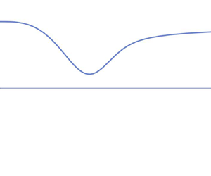
Figure 1 gives a graphical representation of the three presented Stokes shift parameters: the full 2-D version (2.26), the 1-D solution (3.1), and the D–S based solution (3.2). We also added a dotted line to represent the regular terms, given by the first term in (2.26) and (3.1), i.e. the original Stokes dispersion correction in the absence of mean flow (Whitham Reference Whitham1974, (13.123)).

Figure 1. Depth dependence of the nonlinear frequency shift parameter  $\gamma$ given by various formulations: dotted line for ‘regular’ terms only, solid line for full 2-D (2.26), blue dash-dotted line for 1-D (3.1), orange dash-dotted line for D–S (3.2) with $\rho =0.01$, and orange dashed line for D–S (3.2) with $\rho =1.00$. The abscissa is stretched with a cubic power law.
At  $kh\approx 1.363$, the 1-D formula (3.1) presents the well-known sign change of the 1-D nonlinear coefficient, which becomes negative in shallower waters. Its value is $-9/16$ at $kh=0$. The deviation from the Stokes dispersion (dotted line) whose shallow-water value is $9/16$ is due to the ‘singular terms’. In the 2-D expressions, the ‘singular terms’ do not dominate, especially in shallow water, where their contribution is exactly zero. In (3.2), this happens even admitting very small, but finite, directional spreading. Thus a small but finite relaxation of the strict one-dimensionality, as in the D–S system, leads to a positive value of the frequency correction in relatively shallow waters (in contrast to the strictly 1-D setting).
4. Modulational instability (Class I) of a monochromatic wave
One-dimensional periodic wavetrains are modulationally unstable for  $kh>1.363$ (see e.g. Benjamin Reference Benjamin1967; Hasimoto & Ono Reference Hasimoto and Ono1972; Whitham Reference Whitham1974). This result can also be found by perturbing a monochromatic wave with side-bands aligned with the carrier, and accounting for their evolution in the Zakharov equation (1.1), as shown by Janssen & Onorato (Reference Janssen and Onorato2007).
For the monochromatic solution of (1.1), the sub-harmonics set reduces to the wave-induced current (see § 5). In the 1-D setting, its contribution to the nonlinear dispersion causes a sign change at  $kh=1.363$. This fact suggests that the wave-induced current has a stabilising effect in the shallow-water region (Janssen & Onorato Reference Janssen and Onorato2007). The 1-D characteristic sign change at $kh=1.363$ is absent in the 2-D formulation; see figure 1. Thus the Zakharov equation suggests that the effect of the wave-induced current is not as strong as predicted by 1-D theories. However, since the effect of the wave-induced current is less strong in the 2-D formulation and is not causing sign change, it would be interesting to clarify the role of the sub-harmonic component in the stability of the monochromatic wave solution.
Recall that Hayes (Reference Hayes1973) extended the 1-D stability analysis of Whitham (Reference Whitham1974, Ch. 16) and Lighthill (Reference Lighthill1965) to two dimensions. The Hayes–Whitham–Lighthill approach relies on the existence of a variational principle fully describing the gravity-wave problem (Whitham Reference Whitham1967). To study the stability of a periodic wavetrain, the solution is perturbed in amplitude, frequency and wavenumber with a small modulation (Hayes Reference Hayes1973, § 4). The result is that in a fully 2-D system, due to oblique perturbations, the Stokes wave is unstable also for  $kh<1.363$, but unconditionally stable for $kh<0.380$. Exactly the same result was found by Davey & Stewartson (Reference Davey and Stewartson1974) (see also Djordjevic & Redekopp Reference Djordjevic and Redekopp1977). We wish to check if the same applies for the monochromatic solution of the Zakharov equation.
The stability of a uniform wavetrain is governed by (6.8) of Hayes (Reference Hayes1973), which is identical to (3.9) in Davey & Stewartson (Reference Davey and Stewartson1974). In order to facilitate the analysis that follows, we rewrite these results in our notation (see Appendix C for details). The growth rate of the modulations of a Stokes wave with wavelength  $2{\rm \pi} /k$ travelling at depth $h$ can be expressed as
 \begin{equation} \sigma^2_{Hay} \propto G(kh,\theta)\,L(kh,\theta), \end{equation}
where  $G$ is termed the ‘dispersion form’ (Hayes Reference Hayes1973, (6.11)) and equals
 \begin{equation} G(kh,\theta) = \frac{c_g}{k}(1-\cos^2{\theta}) + \frac{\partial c_g}{\partial k} \cos^2{\theta}, \end{equation}
and  $L$ is the ‘effective hardness parameter’ (Hayes Reference Hayes1973, (6.10)) matching
 \begin{align}
L(kh,\theta) &= \frac{9 \tau^4 -10 \tau^2
+ 9}{8 \tau^3} - \frac{c_s^2}{4 ( c_s^2-c_g^2\cos^2{\theta})}\nonumber\\
&\quad \times \left\{ \frac{(1-\tau^2)^2}{\tau} + \left[
\frac{4 \mathrm{g} c_g}{\omega c_s^2}(1-\tau^2)
+ \frac{4}{kh} \right] \cos^2{\theta} \right\}.
\end{align}
\begin{align}
L(kh,\theta) &= \frac{9 \tau^4 -10 \tau^2
+ 9}{8 \tau^3} - \frac{c_s^2}{4 ( c_s^2-c_g^2\cos^2{\theta})}\nonumber\\
&\quad \times \left\{ \frac{(1-\tau^2)^2}{\tau} + \left[
\frac{4 \mathrm{g} c_g}{\omega c_s^2}(1-\tau^2)
+ \frac{4}{kh} \right] \cos^2{\theta} \right\}.
\end{align}
In the equations above,  $\theta$ is the relative direction (with respect to the main wavefront) of the initially small perturbation. As deduced originally by Hayes (Reference Hayes1973) and also found by Janssen & Onorato (Reference Janssen and Onorato2007), from (4.1) with $\theta =n{\rm \pi}$, $n\in \mathbb {Z}$, we recover the stability condition of a monochromatic wave in a pure 1-D system matching the well-established Whitham result (see Whitham Reference Whitham1974, Ch. 16). The marginal stability line $L=0$ cuts the $\theta =n{\rm \pi}$ branches at $kh\approx 1.363$.
In our linear stability analysis, we account for side-band perturbations following Crawford et al. (Reference Crawford, Lake, Saffman and Yuen1981), hence we consider
 \begin{equation} b(\boldsymbol{k}_1) = b_0 \delta_1^0 + \epsilon b_{-} \delta_1^{-} + \epsilon b_{+} \delta_1^{+}, \end{equation}
with  $\epsilon$ being a small ordering parameter, and the choice of wave vectors
 \begin{equation} \boldsymbol{k}_{{\pm}} = \boldsymbol{k}_0 \pm \boldsymbol{\kappa} \end{equation}
identifying the simplest Class I instability triplet  $2\boldsymbol {k}_0=\boldsymbol {k}_+ + \boldsymbol {k}_-$.
On substituting the ansatz (4.4) into (1.1), neglecting  $\epsilon ^2$ terms, and properly treating the arising residual Dirac-delta functions (as done in § 2.1), one finds that the system admits solutions of the type
 \begin{equation} b_{0} = \beta_0\,\mathrm{e}^{-\mathrm{i} \varOmega t} ,\quad b_{+} = \beta_{+}\,\mathrm{e}^{-\mathrm{i} ( \varOmega_{+} + \sigma) t} ,\quad b_{-} = \beta_{-}\,\mathrm{e}^{-\mathrm{i} ( \varOmega_{-} - \sigma^{*}) t} ,\quad \frac{\mathrm{d}}{\mathrm{d} t} \beta_i = 0, \end{equation}
where
 $$\begin{gather} \varOmega = \omega_0 + \tilde{T}_{0} \left\lvert \beta \right\rvert^2, \end{gather}$$
 $$\begin{gather}\varOmega_{{\pm}} = \omega_{{\pm}} + \tfrac{1}{2} \varDelta_{0,0}^{+,-} + ( \tilde{T}_0 \pm \tilde{T}_{0,+} \mp \tilde{T}_{0,-} ) \left\lvert \beta \right\rvert^2 \end{gather}$$
and
 \begin{equation} \sigma^2 = \left[ \tfrac{1}{2}\varDelta_{+,-}^{0,0} + (\tilde{T}_{0,+} + \tilde{T}_{0,-} - \tilde{T}_{0}) \left\lvert \beta \right\rvert^2 \right]^2 - (T_{+,-}^{0,0})^2 \left\lvert \beta \right\rvert^4. \end{equation}
 In (4.7) and (4.8), the objects  $\tilde {T}_{0}$ and $\tilde {T}_{0,\pm }$ are the trivial-resonance integrals given by (2.18) and (B14), respectively, and $\varDelta _{+,-}^{0,0}=\omega _+ + \omega _- -2\omega _0$. The stability of the side-band perturbations is thus governed by the balance between the off-resonant interaction among the three modes $T_{+,-}^{0,0}$ (the last term in the equation above) and a frequency detuning, including the ‘trivial-resonance’ terms.
Hayes–Whitham–Lighthill perturbations can be considered as side-band perturbations in a limit sense (Crawford et al. Reference Crawford, Lake, Saffman and Yuen1981), that is, with an eye to (4.5), for small  $\kappa /k$, i.e. for side-bands representing very-long-wave modulations. For $\kappa /k=0$, (4.8) predicts no instability, i.e. $\sigma ^2=0$. It is easy to see that $\varDelta _{+,-}^{0,0}=\omega _+ + \omega _- -2\omega$ vanishes. In order to see that the remaining term (proportional to $\beta ^2$) also vanishes, one has to recall the expressions (2.19) and (B16). After noticing that the ‘regular terms’ cancel each other, we have
 \begin{align} & \lim_{\kappa}(\tilde{T}_{0,+} + \tilde{T}_{0,-} - \tilde{T}_{0} - T_{+,-}^{0,0} ) \nonumber\\ &\qquad = \lim_{\kappa}( S_{0,+}^{+,0} + \tilde{S}_{0,+} + S_{0,-}^{-,0} + \tilde{S}_{0,-} - 2 \tilde{S}_{0} - 2 S_{+,-}^{0,0} ) = 0, \end{align}
since for symmetry reasons,  $\lim _{\kappa } S_{0,+}^{+,0} = \lim _{\kappa } S_{0,-}^{-,0} = \lim _{\kappa } S_{+,-}^{0,0}$, which is represented by the integrand of (2.21), and $\lim _{\kappa } \tilde {S}_{0,\pm } = \tilde {S}_{0}$ (see § B.4).
We thus have to compute the higher-order terms in the Maclaurin expansion for  $\kappa$, i.e. $\boldsymbol {\kappa }=\kappa [\cos \theta, \sin \theta ]$. At first order, we find only terms proportional to $\left \lvert \beta \right \rvert ^4$, since the multipliers of $\left \lvert \beta \right \rvert ^0$ and $\left \lvert \beta \right \rvert ^2$ are zero. At second order, the multiplier of $\left \lvert \beta \right \rvert ^0$ is zero, while the multiplier of $\left \lvert \beta \right \rvert ^2$ reads
 \begin{align} & \lim_{\kappa\rightarrow 0} \left[ \left(\frac{\partial^2}{\partial \kappa^2}\varDelta_{+,-}^{0,0}\right) (\tilde{T}_{0,+} + \tilde{T}_{0,-} - \tilde{T}_{0}) \right] \nonumber\\ &\quad = 2 G(kh,\theta) [ 2 H_{0,0}^{0,0} + R_{0,0}^{0,0} + \lim_{\kappa\rightarrow 0} (S_{0,+}^{+,0} + \tilde{S}_{0,+} + S_{0,-}^{-,0} + \tilde{S}_{0,-} - 2 \tilde{S}_{0} ) ] \nonumber\\ &\quad = 2 G(kh,\theta) [ 2 H_{0,0}^{0,0} + R_{0,0}^{0,0} + 2 \lim_{\kappa\rightarrow 0} S_{0,+}^{+,0} (\kappa,\theta)] = \frac{k^3}{2 {\rm \pi}^2}\, G(kh,\theta)\,L(kh,\theta). \end{align}
 Putting all this together, disregarding the contribution of  $\left \lvert \beta \right \rvert ^4$ terms, and recalling the surface elevation amplitude $\eta =\left \lvert \beta \right \rvert \sqrt {\omega }/({\rm \pi} \sqrt {2\mathrm {g}})$, we have
 \begin{equation} \sigma^2 = \kappa^2 (k \eta)^2\,\frac{\omega}{2 \tau}\,G(kh,\theta)\, L(kh,\theta) + O[\kappa (k \eta)^4] + O(\kappa^3) . \end{equation}
The leading term behaviour is exactly that predicted by (4.1), i.e. by Hayes (Reference Hayes1973) and Davey & Stewartson (Reference Davey and Stewartson1974). This behaviour dominates, provided that the steepness of the carrier is small enough.
Note that in (4.10), we have used the fact  $\lim _{\kappa } \tilde {S}_{0,\pm } = \tilde {S}_{0}$, i.e. $\lim _{\kappa } \tilde {T}_{0,\pm } = \tilde {T}_{0}$ (see § B.4). As a result, in the limit for small $\kappa$, the self-interaction integral $\tilde {T}_{0}$, given by (2.18), does not contribute to the growth rate of the sidebands. In turn, the growth rate is determined by $L$ given by (4.3), which is the integrand of (2.18).
5. Surface elevation and potential
The simplest solution of the Zakharov equation (1.1) is the monochromatic wave (2.6a), (2.6b), which gives us a solution in terms of canonical variables  $b(\boldsymbol k, t)$. Combining the two canonical transformations, (A4a,b) and (A3), we return to the original physical variables of free surface elevation $\zeta$ and potential at the surface $\psi$. That is, we find the Fourier-transformed elevation (B1) and the potential (B3) evaluated at the free surface.
5.1. Free surface
The free surface can be recovered directly from (B1) via inverse Fourier transform according to (A7a,b). After invoking the ansatz (2.1) and the solution (2.6a), we obtain the well-known Stokes expansion in terms of the generalised Stokes number
 \begin{equation} \hat{\mathcal{U}} = \frac{k\eta}{\tau^3}, \end{equation}
that is,
 \begin{equation} \frac{\zeta(\boldsymbol{x})}{\eta} ={-} Z_0 \hat{\mathcal{U}} + (1 - Z_1 \hat{\mathcal{U}}^2) \cos{(\mu)} + Z_2 \hat{\mathcal{U}} \cos{(2 \mu)} + Z_3 \hat{\mathcal{U}}^2 \cos{(3 \mu)}, \end{equation}
where  $\eta$ is the amplitude of the free mode,
 \begin{equation} \mu = \boldsymbol{k}\,\boldsymbol{\cdot}\,\boldsymbol{x} - \varOmega t, \end{equation}
and
 $$\begin{gather} Z_0 = \frac{c_g c_p \tau^2}{ 4 ( c_s^2 - c_g^2 )} \left[ 2 J^{2,0} + \frac{c_s^2}{c_p c_g} (1 - \tau^2) J^{0,0} \right], \end{gather}$$
 $$\begin{gather}Z_1 = \tfrac{1}{32} [ (3-\tau^2)^2 + 8 \tau^2 (1-\tau^2) Z_0 ], \end{gather}$$
 $$\begin{gather}Z_2 = \tfrac{1}{4} (3-\tau^2), \end{gather}$$
 $$\begin{gather}Z_3 = \tfrac{3}{64} (3-\tau^2) (3+\tau^4) \end{gather}$$
are the coefficients plotted in figure 2.

Figure 2. Coefficients of the Stokes series (5.2). In shallow water, the correction to the surface elevation  $Z_0$ is one order of magnitude ( $kh$) smaller than the other multipliers, and also smaller than the 1-D solution ( $Z_{0,1D}$).
The expressions coincide with the findings of Janssen (Reference Janssen2009), except for the mean set-down  $Z_0$. The Janssen (Reference Janssen2009) formula can be obtained from the above $Z_0$ requiring the narrow-band approximation, i.e. by restricting the solution to the 1-D setting (in practice substituting $J^{2n,0}=1$). In order to compute $Z_0$, we have to compute an integral around a singularity, thus using the same technique adopted for the calculation of the self-interaction kernel (see § 2.2).
The 2-D mean set-down turns out to be small compared to the other second-order contribution. In the 1-D environment, the shallow-water mean flow is as big as the amplitude of the second bound harmonic, while in two dimensions,  $Z_0/Z_2\rightarrow kh$.
5.2. Potential
In the evaluation of the potential, we need to take the inverse transform ((4.1) in Krasitskii Reference Krasitskii1994)
 \begin{equation} \phi(\boldsymbol{x},z,t) = \frac{1}{2{\rm \pi}}\int \hat{\phi}_1\,\frac{\cosh{\left[k (h+z)\right]}}{\sinh{k h}}\,\mathrm{e}^{\mathrm{i}\boldsymbol{k}\,\boldsymbol{\cdot}\, \boldsymbol{x}} \,\mathrm{d}\boldsymbol{k} \end{equation}
of the expansion (A5), after plugging in (B1) and (B3). At  $z=0$, the transformation (5.5) is just the inverse Fourier transform of (A5). Again, invoking the ansatz (2.1) and the solution (2.6a), we find, finally,
 \begin{equation} \frac{\omega}{\mathrm{g} \eta}\,\phi(\boldsymbol{x},0,t) = \varPi_0 \hat{\mathcal{U}}\,\frac{x}{h} + (1 - \varPi_1 \hat{\mathcal{U}}^2) \sin{\mu} + \varPi_2 \hat{\mathcal{U}} \sin{2 \mu} + \varPi_3 \hat{\mathcal{U}}^2 \sin{3 \mu}, \end{equation}
where
 $$\begin{gather} \varPi_0 = \frac{c_s^2 \tau^3}{4 ( c_s^2 - c_g^2 )} \left[ \frac{c_g}{c_p} ( 1-\tau^2 ) + 2 \right] J^{2,0}, \end{gather}$$
 $$\begin{gather}\varPi_1 = \frac{1}{32}\,\frac{1}{1+\tau^2} ( 9 + 9 \tau^2 + 14 \tau^4 - 46 \tau^8 ) + \frac{\tau^5}{2 kh} ( 1 - \tau^2 - 2 kh \tau ) W_2, \end{gather}$$
 $$\begin{gather}\varPi_2 = \tfrac{3}{8} ( 1 - \tau^2 ) ( 1 + \tau^2 ), \end{gather}$$
 $$\begin{gather}\varPi_3 = \tfrac{1}{64} (1-\tau^2) (1+3\tau^2) (9 - 13\tau^2), \end{gather}$$
with
 \begin{equation} W_2 = \frac{c_s^2}{8 (c_s^2-c_g^2)} \left[(1-\tau^2) J^{0,0} + \frac{2 c_g c_p}{c_s^2}\,J^{2,0}\right]. \end{equation}
For the details on the calculation of the mean motion  $\varPi _0$, see § B.3.
6. Concluding remarks
It has been known for more than forty years that in finite-depth water, the kernels of the Zakharov equation and of the associated canonical transformation are singular (Herterich & Hasselmann Reference Herterich and Hasselmann1980). Here, by focusing on the simplest solution of the Zakharov equation, we show that it does not matter whether the kernels are singular, since, upon treating the Dirac- $\delta$ correctly, the integrals involving the singularities are evaluated uniquely, thus the theory is self-sufficient. The key conclusion is that both the four-wave Zakharov equation and the associated canonical transformations are only apparently singular. This means that it is now straightforward to extend to finite-depth waters the efficient way of modelling of all aspects of weakly nonlinear wave dynamics based on the Zakharov equation and the associated canonical transformations, which proved to be so fruitful for deep water (e.g. Annenkov & Shrira Reference Annenkov and Shrira2001, Reference Annenkov and Shrira2013, Reference Annenkov and Shrira2018; Janssen Reference Janssen2003, Reference Janssen2004, Reference Janssen2009). The explicit expressions for the interaction kernels and the associated canonical transformations have been established by Krasitskii (Reference Krasitskii1990, Reference Krasitskii1994) more than thirty years ago.
The validity of the proposed way of handling the finite-depth Zakharov equation has been verified by considering several examples that have been solved earlier employing the Euler equations. In particular, in § 4 concerned with the finite-depth modulational instability, we show that in the limit of very-long-wave perturbations, the stability analysis of the monochromatic solution obtained employing the Zakharov equation yields the same predictions as in Hayes (Reference Hayes1973): that is, periodic long-crested waves are modulationally stable if  $kh<1.363$, but only for perturbations aligned with the carrier.
We recall that all this proceeds from the continuum Hamiltonian theory of water waves that describes the full 2-D initial-value problem on the infinite plane. The results, of course, inherit all the limitations of the Hamiltonian expansion for small depths and finite surface gradients. The Stokes series parameter  $\hat {\mathcal {U}}$ (see (5.1)) indicates once again that in relatively shallow waters, the theory loses meaning if the steepness is $O(kh)^3$. With respect to other solutions, however, the wave-induced flow and the mean-level correction are bounded even if $k\eta \sim (kh)^2$. What is worth emphasizing is that, even in shallow waters, a small increase in steepness corresponds to an increase of the phase celerity. This is the opposite of what is predicted by the Whitham variational principle approach (Whitham Reference Whitham1974, Ch. 6), but is in line with a more intuitive concept that higher waves travel faster. Some 1-D solutions allow a freedom of choice for some parameters, connected to the reference water level and the mean flow, allowing for a wider range of nonlinear corrections to the phase celerity (Fenton Reference Fenton1985; Creedon, Deconinck & Trichtchenko Reference Creedon, Deconinck and Trichtchenko2022). These discrepancies deserve special attention and more detailed examination, since at first glance it seems that different but equally acceptable approaches to the same problem end up describing different physics.
The limitations of the Zakharov equation in shallow water are well known: for sufficiently shallow water and steep waves, the canonical transformation diverges, since exclusion of near-resonant triad interactions becomes impossible. Regimes of nonlinear wave dynamics where such triads are dominant are also possible to describe within the framework of a different Zakharov equation with quadratic nonlinearity (e.g. Vrecica & Toledo Reference Vrecica and Toledo2019). However, a consideration of such nonlinear regimes is beyond the scope of this study.
Although this work is devoted exclusively to water waves, similar Zakharov equations emerge in many branches of physics (see e.g. Zakharov et al. Reference Zakharov, L'vov and Falkovich1992), and the same difficulties have to be common. The proposed way of handling the singularities in the kernels is generic, and we expect its use to not be confined to water waves.
We reiterate our main conclusion: we now have a tool that fully describes 2-D weakly nonlinear waves in waters of intermediate depth, and since we understand all the limitations of this approach, we know a priori the allowed range of water depth and wave steepness. Thus it has become straightforward to extend to intermediate waters the deep-water findings and techniques based on properties of the Zakharov equation and the associated canonical transformations.
Acknowledgements
The authors wish to thank S. Annenkov for initiating their interaction on this topic, and the three anonymous referees for thought-stimulating comments. P.P. also wishes to thank D. Maestrini, M. Onorato and P. Janssen for their fruitful suggestions during the early stages of the work.
Declaration of interests
The authors report no conflict of interest.
Appendix A. Zakharov Hamiltonian formulation
A.1. Canonical transformations
The equation of motion (1.1) is one of the two conjugate Hamilton equations
 \begin{equation} \mathrm{i}\,\frac{\mathrm{d} b}{\mathrm{d} t} = \frac{\delta\,\mathcal{H}(b,b^*)}{\delta b^*}, \end{equation}
where  $\mathcal {H}$ is the reduced Hamiltonian
 \begin{equation} \mathcal{H} = \int \omega_1 b_1 b_2^* \delta_1^2 \,\mathrm{d}\boldsymbol{k}_{1,2} + \int T_{1,2}^{3,4} b_1^* b_2^* b_3 b_4 \delta_{1,2}^{3,4} \,\mathrm{d}\boldsymbol{k}_{1,2}. \end{equation}
The latter is derived by the one corresponding to the full  $\mathcal {H}(a,a^*)$ through the power series transformation
 \begin{align} a_1 &= b_1 + \int B_{1,2,3} b_2^* b_3^* \delta_{1,2,3} \,\mathrm{d} \boldsymbol{k}_{2,3} + \int B_{1,2}^{3} b_2^* b_3 \delta_{1,2}^{3} \,\mathrm{d} \boldsymbol{k}_{2,3} + \int B_{1}^{2,3} b_2 b_3 \delta_{1}^{2,3} \,\mathrm{d} \boldsymbol{k}_{2,3} \nonumber\\ &\quad + \int B_{1,2,3,4} b_2^* b_3^* b_4^* \delta_{1,2,3,4} \,\mathrm{d} \boldsymbol{k}_{2,3,4} + \int B_{1,2,3}^{4} b_2^* b_3^* b_4 \delta_{1,2,3}^{4} \,\mathrm{d} \boldsymbol{k}_{2,3,4} \nonumber\\ &\quad + \int B_{1,2}^{3,4} b_2^* b_3 b_4 \delta_{1,2}^{3,4} \,\mathrm{d} \boldsymbol{k}_{2,3,4} + \int B_{1}^{2,3,4} b_2 b_3 b_4 \delta_{1}^{2,3,4} \,\mathrm{d} \boldsymbol{k}_{2,3,4}. \end{align}
The observable wave action  $a$ is given by
 \begin{equation} \hat{\zeta}_1 = M_1 \left(a_1 + a_{{-}1}^*\right),\quad \mathrm{i} \hat{\psi}_1 = N_1 \left(a_1 - a_{{-}1}^*\right), \end{equation}
where  $\hat {\zeta }$ is the Fourier transformed free-surface elevation, and the potential calculated at the free surface $\hat {\phi }$ has to be recovered from the coordinate $\hat {\psi }$ via the transformation (see Krasitskii Reference Krasitskii1994)
 \begin{equation} \frac{\hat{\phi}_1}{\tau_1} = \hat{\psi}_1 - \frac{1}{2{\rm \pi}}\int k_2 \tau_2 \hat{\psi}_2 \hat{\zeta}_3 \delta_{1}^{2,3} \,\mathrm{d} \boldsymbol{k}_{2,3} - \frac{1}{(2{\rm \pi})^2}\int \varPhi_{1,2}^{3,4} \hat{\psi}_2 \hat{\zeta}_3 \hat{\zeta}_4 \delta_{1}^{2,3,4} \,\mathrm{d} \boldsymbol{k}_{2,3,4}, \end{equation}
where
 \begin{equation} \varPhi_{1,2}^{3,4} = \tfrac{1}{2}\left[k_2^2 - q_2 ( q_{1-3} + q_{1-4})\right]. \end{equation}
The inverse Fourier transforms are
 \begin{equation} \zeta = \frac{1}{2{\rm \pi}}\int\hat{\zeta}\,\mathrm{e}^{\mathrm{i}\boldsymbol{k}\,\boldsymbol{\cdot}\,\boldsymbol{x}} \,\mathrm{d}\boldsymbol{k},\quad \psi = \frac{1}{2{\rm \pi}}\int\hat{\psi}\,\mathrm{e}^{\mathrm{i}\boldsymbol{k}\,\boldsymbol{\cdot}\,\boldsymbol{x}} \,\mathrm{d}\boldsymbol{k}. \end{equation}
All three transformations are canonical, in the sense that the motion (A1) corresponds, for example, to the coupled equations
 \begin{equation} \frac{\mathrm{d} \zeta}{\mathrm{d} t} = \frac{\delta\,\mathcal{H}\left(\zeta,\phi\right)}{\delta \phi},\quad \frac{\mathrm{d} \phi}{\mathrm{d} t} ={-}\frac{\delta\,\mathcal{H}\left(\zeta,\phi\right)}{\delta \zeta}, \end{equation}
where  $\mathcal {H}(\zeta,\phi )$ is the third-order (in wave steepness) truncation of the original Hamiltonian.
A.2. Kernels
In order to perform the evolution calculations, one needs
 \begin{equation} T_{1,2}^{3,4} = 2 H_{1,2}^{3,4} + R_{1,2}^{3,4} + S_{1,2}^{3,4} + S_{1,2}^{4,3}, \end{equation}
where
 $$\begin{gather} R_{1,2}^{3,4} = 9 \left( \frac{1}{\varDelta^{1,2,1+2}} + \frac{1}{\varDelta^{3,4,3+4}}\right) H_{{-}1-2,1,2} H_{{-}3-4,3,4} + \left( \frac{1}{\varDelta^{1+2}_{1,2}} + \frac{1}{\varDelta^{3+4}_{3,4}} \right) H_{1+2}^{1,2} H_{3+4}^{3,4}, \end{gather}$$
 $$\begin{gather}S_{1,2}^{3,4} = \left( \frac{1}{\varDelta_{1}^{3,1-3}} + \frac{1}{\varDelta_{4}^{2,4-2}} \right) H_{1}^{3,1-3} H_{4}^{2,4-2} + \left( \frac{1}{\varDelta_{3}^{1,3-1}} + \frac{1}{\varDelta_{2}^{4,2-4}} \right) H_{3}^{1,3-1} H_{2}^{4,2-4}. \end{gather}$$
The transformation (A3) requires
 $$\begin{gather} B_{1,2,3} ={-}3\,\frac{H_{1,2,3}}{\varDelta_{1,2,3}}, \end{gather}$$
 $$\begin{gather}B_1^{2,3} ={-}\frac{H_1^{2,3}}{\varDelta_1^{2,3}} \end{gather}$$
and
 \begin{align} B_{1,2,3,4}&={-}\frac{1}{\varDelta_{1,2,3,4}} \left[ \frac{2}{3}\left( 3 H_{{-}1-2,1,2} B_{3+4}^{3,4} + 3 H_{{-}1-3,1,3}B_{2+4}^{2,4} + 3 H_{{-}1-4,1,4} B_{2+3}^{2,3}\right.\right.\nonumber\\ &\quad \left.\left. {} +H_{1+2}^{1,2} B_{{-}3-4,3,4} + H_{1+3}^{1,3} B_{{-}2-4,2,4}+ H_{1+4}^{1,4} B_{{-}2-3,2,3} \right) + 4 H_{1,2,3,4}\vphantom{\left[ \frac{2}{3}\left( 3 H_{{-}1-2,1,2} B_{3+4}^{3,4} + 3 H_{{-}1-3,1,3}B_{2+4}^{2,4} + 3 H_{{-}1-4,1,4} B_{2+3}^{2,3} \right.\right.}\right], \end{align}
 \begin{align} B_{1,2,3}^4 &={-}\frac{1}{\varDelta_{1,2,3}^{4}} \left[ 2 \left( H_{4}^{1,4-1} B_{2+3}^{2,3} - H_{1+2}^{1,2} B_{4}^{3,4-3} - H_{1+3}^{1,3} B_{4}^{2,4-2} \right.\right.\nonumber\\ &\quad \left.\left. {}- 3 H_{1,2,-1-2} B_{3}^{4,3-4} - 3 H_{1,3,-1-3} B_{2}^{4,2-4} + H_{1}^{4,1-4} B_{2,3,-2-3} \right) + 3 H_{4}^{1,2,3} \right], \end{align}
 \begin{align} B_{1,2}^{3,4} &= B_{1,2,-1-2} B_{3,4,-3-4} - B_{1+2}^{1,2} B_{3+4}^{3,4} \nonumber\\ &\quad + B_{4}^{1,4-1} B_{2}^{3,2-3} - B_{1}^{4,1-4} B_{3}^{2,3-2} + B_{3}^{1,3-1} B_{2}^{4,2-4} - B_{1}^{3,1-3} B_{4}^{2,4-2}, \end{align}
 \begin{align} B_{1}^{2,3,4}&={-}\frac{1}{\varDelta_{1}^{2,3,4}} \left[ \frac{2}{3}\left( H_{1}^{2,1-2} B_{3+4}^{3,4} + H_{1}^{3,1-3}B_{2+4}^{2,4} + H_{1}^{4,1-4} B_{2+3}^{2,3} \right.\right.\nonumber\\ &\quad \left. \left. {}+ H_{2}^{1,2-1}B_{3,4,-3-4} + H_{3}^{1,3-1} B_{2,4,-2-4} + H_{4}^{1,4-1}B_{2,3,-2-3} \right) + H_{1}^{2,3,4} \vphantom{\left[ \frac{2}{3}\left( 3 H_{{-}1-2,1,2} B_{3+4}^{3,4} + 3 H_{{-}1-3,1,3}B_{2+4}^{2,4} + 3 H_{{-}1-4,1,4} B_{2+3}^{2,3} \right.\right.}\right]. \end{align}
 The  $H$ elements are the kernels of the linear complex action Hamiltonian $\mathcal {H}(a,a^*)$:
 $$\begin{gather} H_{1,2,3} ={-}\tfrac{1}{3} \left( F_{1,2}^3 + F_{1,3}^2 + F_{2,3}^1 \right), \end{gather}$$
 $$\begin{gather}H_{1}^{2,3} = F_{1,-2}^3 + F_{1,-3}^2 - F_{2,3}^1, \end{gather}$$
 $$\begin{gather}H_{1,2,3,4} ={-}\tfrac{1}{6} \left( F_{1,2}^{3,4} + F_{1,3}^{2,4} + F_{1,4}^{2,3} + F_{2,3}^{1,4} + F_{2,4}^{1,3} + F_{3,4}^{1,2} \right), \end{gather}$$
 $$\begin{gather}H_{1,2}^{3,4} ={-} F_{1,2}^{{-}3,-4} + F_{1,-3}^{2,-4} + F_{1,-4}^{2,-3} + F_{2,-3}^{1,-4} + F_{2,-4}^{1,-3} - F_{3,4}^{{-}1,-2}, \end{gather}$$
 $$\begin{gather}H_{1}^{2,3,4} = \tfrac{2}{3} \left( F_{{-}1,2}^{3,4} + F_{{-}1,3}^{2,4} + F_{{-}1,4}^{2,3} - F_{2,3}^{{-}1,4} - F_{2,4}^{{-}1,3} - F_{3,4}^{{-}1,2} \right), \end{gather}$$
where
 $$\begin{gather} F_{1,2}^{3,4} = N_1 N_2 M_3 M_4 E_{1,2}^{3,4}, \end{gather}$$
 $$\begin{gather}F_{1,2}^{3} = N_1 N_2 M_3 E_{1,2}^{3}, \end{gather}$$
with
 $$\begin{gather} E_{1,2}^{3,4} = \frac{1}{8 (2{\rm \pi})^2}\left[q_1 q_2 \left( q_{1+3} + q_{1+4} + q_{2+3} + q_{2+4} \right) - 2 q_1 k_2^2 - 2 q_2 k_1^2\right], \end{gather}$$
 $$\begin{gather}E_{1,2}^{3} ={-}\frac{1}{2 (2{\rm \pi})}\left( q_1 q_2 + \boldsymbol{k}_1\,\boldsymbol{\cdot}\,\boldsymbol{k}_2\right) \end{gather}$$
being the kernels of  $\mathcal {H}(\hat {\zeta },\hat {\phi })$, and
 \begin{equation} M_1 = \sqrt{\frac{\omega_1}{2\mathrm{g}}},\quad N_1 = \sqrt{\frac{\mathrm{g}}{2\omega_1}},\quad q_1 = k_1 \tau_1 = k_1 \tanh{k_1 h} . \end{equation}
Appendix B. Reconstruction of physical variables
B.1. Free surface
Combining (A3) with (A4a,b), we obtain the free surface, in wavenumber space, in terms of the reduced action  $b$:
$b$:
 \begin{align} \hat{\zeta}_1 &= M_1 ( b_1 + b_{{-}1}^* ) + \int Y_{1,2}^{3} b_2^* b_3 \delta_{1,2}^{3} \,\mathrm{d} \boldsymbol{k}_{2,3} + \int Y_{1,2,3} ( b_2^* b_3^* + b_{{-}2} b_{{-}3} ) \delta_{1,2,3} \,\mathrm{d} \boldsymbol{k}_{2,3} \nonumber\\ &\quad + \int Y_{1,2,3}^{4} ( b_2^* b_3^* b_4 + b_{{-}2} b_{{-}3} b_{{-}4}^* ) \delta_{1,2,3}^{4} \,\mathrm{d} \boldsymbol{k}_{2,3,4} \nonumber\\ &\quad + \int Y_{1,2,3,4} (b_2^* b_3^* b_4^* + b_{{-}2} b_{{-}3} b_{{-}4} ) \delta_{1,2,3,4} \,\mathrm{d} \boldsymbol{k}_{2,3,4}, \end{align}
where
 $$\begin{gather} Y_{1,2,3} = M_1 \left( B_{1,2,3} + B_{{-}1}^{2,3} \right), \end{gather}$$
 $$\begin{gather}Y_{1,2}^{3} = M_1 \left( B_{1,2}^{3} + B_{{-}1,3}^{2} \right), \end{gather}$$
 $$\begin{gather}Y_{1,2,3,4} = M_1 \left( B_{1,2,3,4} + B_{{-}1}^{2,3,4} \right), \end{gather}$$
 $$\begin{gather}Y_{1,2,3}^{4} = M_1 \left( B_{1,2,3}^{4} + B_{{-}1,4}^{2,3} \right). \end{gather}$$
B.2. Potential
Combining (A3) with (A4a,b), we obtain the second canonical variable:
 \begin{align} \mathrm{i}\hat{\psi}_1 &= N_1 \left( b_1 - b_{{-}1}^* \right) + \int X_{1,2}^{3} b_2^* b_3 \delta_{1,2}^{3} \,\mathrm{d} \boldsymbol{k}_{2,3} \nonumber\\ &\quad + \int X_{1,2,3} \left( b_2^* b_3^* - b_{{-}2} b_{{-}3} \right) \delta_{1,2,3} \,\mathrm{d} \boldsymbol{k}_{2,3} \nonumber\\ &\quad + \int X_{1,2,3,4} \left( b_2^* b_3^* b_4^* - b_{{-}2} b_{{-}3} b_{{-}4} \right) \delta_{1,2,3,4} \,\mathrm{d} \boldsymbol{k}_{2,3,4} \nonumber\\ &\quad + \int X_{1,2,3}^{4} \left( b_2^* b_3^* b_4 - b_{{-}2} b_{{-}3} b_{{-}4}^* \right) \delta_{1,2,3}^{4} \,\mathrm{d} \boldsymbol{k}_{2,3,4}, \end{align}
with
 $$\begin{gather} X_{1,2,3} = N_1 \left( B_{1,2,3} - B_{{-}1}^{2,3} \right), \end{gather}$$
 $$\begin{gather}X_{1,2}^{3} = N_1 \left( B_{1,2}^{3} - B_{{-}1,3}^{2} \right), \end{gather}$$
 $$\begin{gather}X_{1,2,3,4} = N_1 \left( B_{1,2,3,4} - B_{{-}1}^{2,3,4} \right), \end{gather}$$
 $$\begin{gather}X_{1,2,3}^{4} = N_1 \left( B_{1,2,3}^{4} - B_{{-}1,4}^{2,3} \right). \end{gather}$$
Plugging (B3) and (B1) into (A5), we have
 \begin{align} \mathrm{i}\,\frac{\hat{\phi}_1}{\tau_1} &= N_1 \left( b_1 - b_{{-}1}^* \right) + \int P_{1,2}^{3} b_2^* b_3 \delta_{1,2}^{3} \,\mathrm{d} \boldsymbol{k}_{2,3} \nonumber\\ &\quad + \int P_{1,2,3} \left( b_2^* b_3^* - b_{{-}2} b_{{-}3} \right) \delta_{1,2,3} \,\mathrm{d} \boldsymbol{k}_{2,3} \nonumber\\ &\quad + \int P_{1,2,3,4} \left( b_2^* b_3^* b_4^* - b_{{-}2} b_{{-}3} b_{{-}4} \right) \delta_{1,2,3,4} \,\mathrm{d} \boldsymbol{k}_{2,3,4} \nonumber\\ &\quad + \int P_{1,2,3}^{4} \left( b_2^* b_3^* b_4 - b_{{-}2} b_{{-}3} b_{{-}4}^* \right) \delta_{1,2,3}^{4} \,\mathrm{d} \boldsymbol{k}_{2,3,4}. \end{align}
After proper symmetrisation, the coefficients are
 \begin{gather} P_{1,2,3} = X_{1,2,3} + \frac{1}{4{\rm \pi}} \left( k_2 \tau_2 N_2 M_3 + k_3 \tau_3 N_3 M_2 \right), \end{gather}
 \begin{gather} P_{1,2}^{3} = X_{1,2}^{3} + \frac{1}{2{\rm \pi}} \left( k_2 \tau_2 N_2 M_3 - k_3 \tau_3 N_3 M_2 \right), \end{gather}
 \begin{align} P_{1,2,3,4}& = X_{1,2,3,4} + \frac{1}{3(2{\rm \pi})^2} \big(N_2 M_3 M_4 \varPhi_{1,-2}^{{-}3,-4} + N_3 M_2 M_4 \varPhi_{1,-3}^{{-}2,-4} + N_4 M_2 M_3 \varPhi_{1,-4}^{{-}2,-3} \big) \nonumber\\ &\quad - \frac{1}{6{\rm \pi}} \left( k_{1+2} \tau_{1+2} M_2 X_{1+2,3,4} - k_2 \tau_2 N_2 Y_{1+2,3,4} \right) \nonumber\\ &\quad - \frac{1}{6{\rm \pi}} \left( k_{1+3} \tau_{1+3} M_3 X_{1+3,2,4} - k_3 \tau_3 N_3 Y_{1+3,2,4} \right) \nonumber\\ &\quad - \frac{1}{6{\rm \pi}} \left( k_{1+4} \tau_{1+4} M_4 X_{1+4,2,3} - k_4 \tau_4 N_4 Y_{1+4,2,3} \right), \end{align}
 \begin{align} P_{1,2,3}^{4} &= X_{1,2,3}^{4} - \frac{1}{2{\rm \pi}} \left( k_{2+3} \tau_{2+3} M_4 X_{{-}2-3,2,3} + k_4 \tau_4 N_4 Y_{{-}2-3,2,3} \right) \nonumber\\ &\quad - \frac{1}{4{\rm \pi}} \big(k_{4-3} \tau_{4-3} M_2 X_{4-3,3}^{4} + k_{4-2} \tau_{4-2} M_3 X_{4-2,2}^{4}\big) \nonumber\\ &\quad + \frac{1}{4{\rm \pi}} \big(k_2 \tau_2 N_2 Y_{4-3,3}^{4} + k_3 \tau_3 N_3 Y_{4-2,2}^{4}\big) \nonumber\\ &\quad + \frac{1}{(2{\rm \pi})^2} \left[ N_2 M_3 M_4 \varPhi_{1,-2}^{{-}3,4} + M_2 N_3 M_4 \varPhi_{1,-3}^{{-}2,4} - M_2 M_3 N_4 \varPhi_{1,4}^{{-}2,-3} \right]. \end{align}
B.3. Mean flow
The evaluation of the mean flow associated with the monochromatic solution is somehow critical, since the kernel is strongly singular. After invoking the monochromatic ansatz, and applying inverse Fourier, the second integral of (B5) becomes
 \begin{align} &\int P_{2,1}^{1+2} \delta_2\,\mathrm{e}^{\mathrm{i} \boldsymbol{k}_2\,\boldsymbol{\cdot}\,\boldsymbol{x}} \,\mathrm{d} \boldsymbol{k}_{2} = \int X_{2,1}^{1+2} \delta_2\,\mathrm{e}^{\mathrm{i} \boldsymbol{k}_2\,\boldsymbol{\cdot}\,\boldsymbol{x}} \,\mathrm{d} \boldsymbol{k}_{2} \nonumber\\ &\qquad + \int \frac{1}{2{\rm \pi}} \left( k_1 \tau_1 N_1 M_{1+2} - k_{1+2} \tau_{1+2} N_{1+2} M_1 \right) \delta_2\,\mathrm{e}^{\mathrm{i} \boldsymbol{k}_2\,\boldsymbol{\cdot}\,\boldsymbol{x}} \,\mathrm{d} \boldsymbol{k}_{2}. \end{align}
The second term is clearly zero, but the first is singular:
 \begin{equation} \lim_{k_2} X_{2,1}^{1+2} \rightarrow \lim_{k_2} \frac{1}{k_2}\,W\,\frac{ \cos{\theta} }{ c_s^2 - c_g^2 \cos^2{\theta} } + \cdots, \end{equation}
with
 \begin{equation} W = \frac{\mathrm{g} k}{4 {\rm \pi}} \left[ \frac{c_g}{c_p} (1-\tau^2) + 2 \right]. \end{equation}
The leading term in (B8) is likely to vanish when taking the directional average, but it is unclear if the Maclaurin expansion exists. Instead of studying the higher-order terms, it is convenient to look directly at the mean flow quantities. By taking the gradient – in Cartesian reference this reads  $\boldsymbol {\nabla }=(\partial _x,\partial _y,\partial _z)$ – of the mean potential, we find the mean velocities
 \begin{equation} \mathrm{i}\,2 {\rm \pi}\left(\bar{u}, \bar{v}, \bar{w}\right) = \boldsymbol{\nabla} \int \tau_2 P_{2,1}^{1+2}\, \frac{\cosh{k_2 \left(z + h\right)}}{\sinh{k_2 h}}\,\delta_2\,\mathrm{e}^{\mathrm{i} \boldsymbol{k}_2\,\boldsymbol{\cdot}\,\boldsymbol{x}} \,\mathrm{d} \boldsymbol{k}_{2}, \end{equation}
which have to be evaluated according to the procedure outlined in § 2.2. Assuming that  $\boldsymbol {k}_1$ is oriented along the abscissa $x$, to lowest order,
 \begin{equation} \boldsymbol{\nabla} \frac{\cosh{k_2 (z + h)}}{\sinh{k_2 h}}\,\mathrm{e}^{\mathrm{i} \boldsymbol{k}_2\,\boldsymbol{\cdot}\,\boldsymbol{x}} = \left(\frac{\mathrm{i}}{h} \cos{\theta}, \frac{\mathrm{i}}{h} \sin{\theta}, k_2\,\frac{z+h}{h} \right), \end{equation}
so that, as expected, the only non-zero contribution is along the main motion  $\boldsymbol {k}_1$:
 \begin{equation} \left(\bar{u}, \bar{v}, \bar{w}\right) = \left( \frac{ W }{ 2 {\rm \pi}( c_s^2 - c_g^2 ) }\, J^{2,0}, 0, 0 \right), \end{equation}
with  $J^{2,0}$ given by (2.24a,b). We can then integrate back to find the mean flow potential and, recalling (B9), define
 \begin{equation} P_{0,1}^1 = \int P_{2,1}^{1+2} \delta_2\,\mathrm{e}^{\mathrm{i} \boldsymbol{k}_2\,\boldsymbol{\cdot}\,\boldsymbol{x}} \,\mathrm{d} \boldsymbol{k}_{2} = \frac{\mathrm{g} k}{4 {\rm \pi} ( c_s^2 - c_g^2)} \left[ \frac{c_g}{c_p} (1-\tau^2) + 2 \right] J^{2,0} x \end{equation}
plus an arbitrary constant. Note that again, the mean motion is similar to the Whitham 1-D finding, except for the multiplier  $J^{2,0}$. This reduces the intensity of the mean flow, in shallow waters, from $O(1)$ in one dimension to $O(kh)$ in two dimensions.
B.4. Explicit expressions for trivial resonances
Finite water depth introduces singularities not only in the motion of the monochromatic wave, but all along the more general wave–wave interactions, that is, the degenerate quartets interactions that one would encounter, for example, studying the evolution of a bi-chromatic wave field. The singularities of the kernel  $T_{1,2}^{3,4}$ lie on the manifold $\boldsymbol {k}_3=\boldsymbol {k}_1$ ( $\boldsymbol {k}_4=\boldsymbol {k}_2$), that is, the object $T_{1,2}^{1,2}$ does not exist. However, whether or not this limit exists is not important. Using the same careful steps as outlined in §§ 2.1 and 2.2, one finds that the generic trivial interactions are to be determined computing the more general integral
 \begin{equation} \tilde{T}_{1,2} = \frac{1}{2{\rm \pi}} \int_{0}^{2{\rm \pi}} \lim_{k_3\rightarrow 0} T_{1+3,2-3}^{1,2}(k_3,\theta_3) \,\mathrm{d} \theta_3 , \end{equation}
and we can then verify that the result of § 2.2 can be obtained in a straightforward way:
 \begin{equation} \tilde{T}_{1} = \lim_{\boldsymbol{k}_2\rightarrow\boldsymbol{k}_1} \tilde{T}_{1,2}, \end{equation}
with  $\tilde {T}_1$ given by (2.18), obviously interchanging the subscripts $0$ and $1$. Substituting (1.2) into (B14), we have
 \begin{equation} \tilde{T}_{1,2} = 2 H_{1,2}^{1,2} + R_{1,2}^{1,2} + S_{1,2}^{2,1} + \tilde{S}_{1,2}, \end{equation}
where
 \begin{equation} \tilde{S}_{1,2} = \frac{1}{2{\rm \pi}} \int_{0}^{2{\rm \pi}} \lim_{k_3\rightarrow 0} S_{1+3,2-3}^{1,2}(k_3,\theta_3) \,\mathrm{d} \theta_3, \end{equation}
and the terms  $H_{1,2}^{1,2}$, $R_{1,2}^{1,2}$ and $S_{1,2}^{2,1}$ exist, in the sense that they can be calculated straightforwardly from the general expressions $H_{1,2}^{3,4}$, $R_{1,2}^{3,4}$ and $S_{1,2}^{4,3}$ (see Appendix A) without passing through a limiting process. We recall that the sum $2 H_{1,2}^{1,2} + R_{1,2}^{1,2}$ in (B16) constitutes the ‘regular part’ of the kernel, equal to the one reported by Stiassnie & Gramstad (Reference Stiassnie and Gramstad2009), and thus, according to Reference Stiassnie and GramstadStiassnie & Gramstad, corresponds to the expression for the Stokes shift given by Madsen & Fuhrman (Reference Madsen and Fuhrman2006).
According to (B17), after making use of the definitions in Appendix A, we find
 \begin{align} &\tilde{S}_{1,2} ={-} \frac{\mathrm{g}}{16 (2{\rm \pi})^2 (c_s^2-c_{g,1}^2)} \left\{ s P_1 P_2 J^{0,0}_{1} + \left[ c_s Q_1 Q_2 \cos{\theta_{1,2}}\right.\right.\nonumber\\ &\quad -\left.\left. c_{g,1} ( P_2 Q_1 - P_1 Q_2 \cos{\theta_{1,2}}) \right] J^{2,0}_{1} \right\} \nonumber\\ &\quad - \frac{\mathrm{g}}{16 (2{\rm \pi})^2 (c_s^2-c_{g,2}^2)} \left\{ c_s P_1 P_2 J^{0,0}_{2} + \left[ c_s Q_1 Q_2 \cos{\theta_{1,2}}\right.\right.\nonumber\\ &\quad - \left.\left.c_{g,2} (P_1 Q_2 - P_2 Q_1 \cos{\theta_{1,2}}) \right] J^{2,0}_{2} \right\}, \end{align}
where  $\theta _{1,2}$ is the angle spanned by $\boldsymbol {k}_1$ rotating anticlockwise over $\boldsymbol {k}_2$,
 \begin{equation} P_i = \frac{k_i^2 \sqrt{c_s}}{\omega_i} (\tau_i^2-1) ,\quad Q_i = \frac{2 k_i}{\sqrt{c_s}} , \end{equation}
and  $J$ is given by (2.24a,b). The expression (B18) corresponds to the directional average, with respect to the angles $\theta _{a3}$ and $\theta _{b3}$, of (5.1) in Stiassnie & Gramstad (Reference Stiassnie and Gramstad2009).
Appendix C. Modulations growth rate equivalence
This appendix shows that (6.8) in Hayes (Reference Hayes1973) as well as (3.9) in Davey & Stewartson (Reference Davey and Stewartson1974) can be rewritten as (4.1).
The right-hand side of (6.8) in Hayes (Reference Hayes1973) gives the growth rate of the modulations in terms of the product of two functions, termed as dispersion and hardness:
 \begin{equation} \sigma^2 \propto \varOmega_A^{\prime} \mathcal{H}_{kk}\colon\boldsymbol{nn}, \end{equation}
where  $\varOmega _A^{\prime }$ is the hardness parameter given by (6.10) in Hayes (Reference Hayes1973):
 \begin{equation} \varOmega_A^{\prime} = \varOmega_A - \left(\frac{k^2}{h}\right) \frac{\mu^2(\mathrm{g} h + 2 C_0 B)+B^2}{\mathrm{g} h -\mu^2 C_0^2}. \end{equation}
Using (6.4d) with (6.3) of Hayes (Reference Hayes1973) to find  $\varOmega _A$, and then, for the second term, (6.5) and (6.6), which is the group celerity, one finds an explicit form for $\varOmega _A^{\prime }$. After recalling from Hayes (Reference Hayes1973) the definition $\mu =\cos \psi$ and substituting $T$ (which stands for $\tanh {kh}$) with $\tau$, and $\psi$ with $\theta$, one finds that $\varOmega _A^{\prime }=L$, with $L$ given by (4.3).
The dispersion parameter, given by (6.11) in Hayes (Reference Hayes1973), is
 \begin{align} \mathcal{H}_{kk}\colon\boldsymbol{nn} &= [ - \tfrac{1}{4}\,k^{{-}2} \omega_0 + \tfrac{1}{2} (2k^{{-}1}-h T^{{-}1}-3 h T) B ] \mu^2 A\nonumber\\ &\quad + [ \tfrac{1}{2}\,k^{{-}2} \omega_0 + k^{{-}1} B ] (1-\mu^2) A, \end{align}
with  $A$ the amplitude of the carrier. Using (6.5) and (6.6) of Hayes (Reference Hayes1973), one finds immediately that the second term in square brackets is half the group celerity divided by $k$, and, with a bit of algebra, can verify that the first term in square brackets is half the derivative of the group celerity with respect to $k$, i.e.
 \begin{equation} \mathcal{H}_{kk}\colon\boldsymbol{nn} = \frac{1}{2}\,A \left[ \frac{\partial c_g}{\partial k}\,\mu^2 + \frac{c_g}{k} (1-\mu^2) \right]. \end{equation}
Therefore, recalling the meaning of  $\mu$, we find $\mathcal {H}_{kk}\colon \boldsymbol {nn}=\tfrac {1}{2} A\,G(kh, \theta )$, with $G$ given by (4.2). This is sufficient to prove that (C1) corresponds to our (4.1).
Also, (3.9) in Davey & Stewartson (Reference Davey and Stewartson1974) gives the growth rate as a product of two functions:
 \begin{equation} \sigma^2 \propto (\lambda l^2 + \mu m^2 ) \left(\nu + \frac{\nu_1 \kappa_1 m^2}{\lambda_1 l^2 + \mu_1 m^2}\right), \end{equation}
with  $l$ and $m$ the wavenumbers of the modulation in their rescaled reference, namely $\zeta =\epsilon (x-c_g t)$ and $\eta =\epsilon y$. The magnitudes of $l$ and $m$ are not prescribed. We can map them in polar coordinates by putting $l^2+m^2=\kappa ^2$, $l/\kappa =\cos {\theta }$ and $m/\kappa =\sin {\theta }$, without making any restriction. Recalling also $\lambda$, $\mu$, $\lambda _1$ and $\mu _1$ from (2.5) in Davey & Stewartson (Reference Davey and Stewartson1974), we find from (C5) that
 \begin{equation} \sigma^2 \propto \frac{1}{2}\,\kappa^2 \left[\frac{\partial c_g}{\partial k} \cos^2{\theta} + \frac{c_g}{k} (1-\cos^2{\theta})\right] \left[ \nu + \frac{\nu_1 \kappa_1 (1-\cos^2{\theta})}{c_s^2-c_g^2 \cos^2{\theta}}\right]. \end{equation}
The first term is clearly the dispersion parameter  $G$ given by (4.2). In order to verify that the last term equals $L$ given by (4.3), one has to invoke $\nu$, $\nu _1$ and $\kappa _1$ from (2.5) in Davey & Stewartson (Reference Davey and Stewartson1974), or the inviscid version of the corresponding (2.17) in Djordjevic & Redekopp (Reference Djordjevic and Redekopp1977), and then rearrange the terms. In both papers, the formulas for $\nu$ and $\nu _1$ are affected by typos, which fortunately are different and can be spotted easily. For the sake of completeness, we report here their correct versions (replacing their $\sigma$ with our $\tau$):
 $$\begin{gather} \nu =\frac{k^4}{4\omega} \left\{ \frac{9-10 \tau^2+9\tau^4}{\tau^2} - \frac{8 c_g^2}{c_s^2-c_g^2} \left[ \left(\frac{c_p}{c_g}\right)^2 + \frac{c_p}{c_g}(1-\tau^2) + \frac{c_s}{4 c_g^2}(1-\tau^2)^2 \right] \right\}, \end{gather}$$
 $$\begin{gather}\nu_1 = \frac{k^4}{\omega} \left[ \frac{c_p}{c_g} + \frac{1}{2} (1-\tau^2) \right], \end{gather}$$
with  $c_p=\omega /k$ and $c_s=\sqrt {\mathrm {g} h}$. Thus (C5) also matches our (4.1).


 Open access