


1. Introduction
The extensive use of composite permeable acoustic materials to reduce the external community noise in modern aircraft (Camussi & Di Marco Reference Camussi and Di Marco2013) could cause a higher transmission to the cabin of the vibration generated by the development of the external flow over the fuselage surface. The cabin noise is a crucial point for aircraft manufacturers because of its impact on passengers comfort and on the crew's health (Mellert et al. Reference Mellert, Baumann, Freese and Weber2008). In the same way, the wall pressure load generated by the external turbulent boundary layer and by the impact of the jet plume over the rear part of the fuselage or on the wing pressure side can cause fatigue problems because of the induced vibrations. Above all, in future configurations, like the blended wing body where the fuselage efficiently shields the jet noise, the jet-induced wall pressure load could significantly stress the aircraft panels (Liebeck Reference Liebeck2002; Salehian & Mankbadi Reference Salehian and Mankbadi2020).
The complications related to jet-induced surface pressure load and to the radiated noise behaviour are further amplified for high-speed propulsion systems. Indeed, the renewed interest in high-speed commercial aircraft impacts flight test procedures to progress and adapt noise certifications to supersonic conditions. To take off and land safely, jet engines for supersonic aircraft require relatively greater thrust, and the engine nacelle diameter must be relatively small, being well integrated into the airframe/wing design to reduce the increased drag. Supersonic jet wing integrated configurations are expected to be louder than subsonic installed configurations, increasing the wall pressure load transmitted inside the fuselage and stressing the wing/fuselage panels with very energetic and frequency localized supersonic effects.
Several investigations carried out on isolated supersonic jets (Powell Reference Powell1953b; Tam Reference Tam1995; Raman Reference Raman1998, Reference Raman1999) clarified the main features of the radiated noise. At off-design conditions, the difference between the jet exit and ambient pressures leads to the generation of a series of shock cells that radiate broadband noise as an effect of their interaction with the jet mixing layer (the so-called broadband shock associated noise, BBSAN). The acoustic feedback loop between the nozzle and the shock cells originates the screech tones that are revealed by the localized peak of the noise spectra (Powell Reference Powell1953b). The screech fundamental tone and its harmonics have a well-defined directivity pattern and the wavelength is related to the shock cell spacing (Powell Reference Powell1953a; Edgington-Mitchell Reference Edgington-Mitchell2019). The results of several experimental studies on the screech phenomenon separated four modes (termed A, B, C and D) characterised by discontinuous changes in frequency and different azimuthal structure of both the sound field and downstream propagating disturbances. For the present nozzle pressure ratios (NPRs), the so called A1 and A2 modes, corresponding to axisymmetric toroidal topologies, are expected to be activated.
Fewer studies have been carried out on installed supersonic jets and the influence of solid boundaries on the aforementioned noise sources is still unclear. Brown, Clem & Fagan (Reference Brown, Clem and Fagan2015) investigated the far-field noise emitted by an installed supersonic round jet, operating in the over-expanded, ideally expanded and under-expanded conditions. They showed that the surface will be effective at reducing the broadband shock noise only if it is long enough to shield the noise produced by the shocks. The impact of the jet-induced wall pressure load over a carrier deck has been investigated using a numerical solver by Liu et al. (Reference Liu, Kailasanath, Heeb, Munday and Gutmark2013), highlighting the influence of reflections on the near-field pressure fluctuations.
The literature survey reveals that experimental studies on wall pressure generated in jet-wing configurations have been limited to sonic or subsonic conditions. Meloni et al. (Reference Meloni, Di Marco, Mancinelli and Camussi2019, Reference Meloni, Di Marco, Mancinelli and Camussi2020a) mocked up the wing with a tangential flat plate and provided models for the pressure auto- and cross-spectra accounting for the effect of the Mach and Reynolds numbers. These models have been applied successfully to more realistic jet-wing configurations, as reported in Meloni et al. (Reference Meloni, Mancinelli, Camussi and Huber2020b, Reference Meloni, Proença, Lawrence and Camussi2021). Recently, Camussi et al. (Reference Camussi, Ahmad, Meloni, de Paola and Di Marco2022) extended the analysis to sonic jets in under-expanded flow conditions highlighting the signature on the wall pressure load of the BBSAN and of the screech tones. However, an extensive analysis that includes the effect of the plate on the screech modes is missing.
The main scope of the present work is to cover the lack of knowledge in the field by investigating wall pressure fluctuations induced by supersonic flows on a rigid surface and by providing a model for their single and multivariate statistical spectral properties. The investigation is carried out around the design jet Mach number (for the considered nozzle,  $M=1.19$ and ${\rm NPR}=2.4$) covering the typical working regimes of supersonic nozzles. The design jet Mach number has been chosen slightly supersonic in order to avoid the effect of the flow temperature as a further parameter. Furthermore, this Mach number is close to the expected conditions for near-term supersonic civil transports where propulsion systems will be obtained by the redesign of low-speed turbofan engines currently in use (see Berton et al. Reference Berton, Huff, Prestianni and Seidel2020).
The wall pressure fluctuations are acquired by a couple of pressure transducers flush mounted on a plate and positioned at different distances from the jet exit. Different jet-plate grazing has been considered by varying the jet-plate distance from between  $H/D=0.75$ and $H/D=2$, where $H$ denotes the radial distance of the plate from the jet axis and $D$ the nozzle exhaust diameter.
Pitot measurements and background oriented schlieren (BOS) flow visualizations have been carried out to provide an overall characterisation of the aerodynamic field and of the jet plume spatial evolution, along with a qualitative estimation of the flow distortion due to the presence of the rigid plate.
Multivariate statistical analyses were computed in the spectral domain to characterise in detail the wall pressure fluctuations and to identify the signatures of the typical noise sources observed in supersonic jets, namely BBSAN and screech.
The spectral properties are interpreted in the framework of existing models (e.g. Corcos Reference Corcos1964; Rozenberg, Robert & Moreau Reference Rozenberg, Robert and Moreau2012; Meloni et al. Reference Meloni, Di Marco, Mancinelli and Camussi2019) that, for the present complex configuration, are shown to be uneffective in predicting the pressure auto- and cross-spectra. Also, the use of linear stability analysis to predict the evolution of the screech modes can be very difficult because of the presence of the plate that breaks the axisymmetry of the flow.
In order to manage the intrinsic complexity and richness of the wall pressure spectral content, the modelling strategy we follow relies on the use of artificial intelligence techniques that are able to provide surrogate models. Machine learning techniques have been successfully exploited in similar configurations, for example, to correlate computational fluid dynamics data to the jet acoustic response (Shah Reference Shah2019) or to successfully predict the far-field noise spectra produced by supersonic jets with different nozzle shapes located near a surface (Brown et al. Reference Brown, Dowdall, Whiteaker and McIntyre2020). The predictive surrogate model developed therein is based on artificial neural networks (ANNs), a versatile tool that can be used to represent phenomena when it is not possible to assess a physical model. The dichotomy between biological neurons and mathematical processes has been investigated in the 1940s (McCulloch & Pitts Reference McCulloch and Pitts1943; Hebb Reference Hebb1949), but the theoretical layout of complex multilayer structures was developed within the last 50 years (Ivakhnenko Reference Ivakhnenko1967, Reference Ivakhnenko1973) thanks to the increase in computing resources. The ANNs are widely used in computer vision and speech recognition (Safran & Shamir Reference Safran and Shamir2017) and, more recently, are also being employed in the construction of surrogate models in the aeroacoustic field, alongside the well-assessed radial basis functions dynamic models (Centracchio et al. Reference Centracchio, Burghignoli, Palma, Cioffi and Iemma2021b; Burghignoli et al. Reference Burghignoli, Rossetti, Centracchio, Palma and Iemma2022).
Artificial neural networks are nowadays applied extensively also in fluid mechanics. As examples, Kim & Lee (Reference Kim and Lee2020) used the ANNs with a deep learning approach based only on wall information to predict turbulent heat transfer. In the work of Lee & You (Reference Lee and You2019) the unsteady flow fields over a circular cylinder are used for training four different deep learning networks providing reliable predictions. Le Clainche, Rosti & Brandt (Reference Le Clainche, Rosti and Brandt2022) presented a data-driven model applied to approximate the statistics of the averaged wall-shear stress in a turbulent channel flow over a porous wall. Centracchio et al. (Reference Centracchio, Meloni, Jawahar, Azarpeyvand, Camussi and Iemma2022) recently proposed a data-driven nonlinear model based on ANNs to describe and predict the noise emitted by a single stream jet in under-expanded conditions.
In the present paper an optimized network topology for the wall pressure fluctuating field has been built considering all the experimental parameters (i.e. axial position of the probes, radial position of the plate and NPR) and using the available data to train and validate the network. The network topology is selected by means of a tailored deterministic minimisation process, which aims at finding the optimal (or near-optimal) architecture in terms of a number of hidden layers, neurons per layer and activations. The optimization algorithm is coupled with a suitable self-tuning scheme to ensure efficient network training. In addition, using the spatial correlation, the model provides the uncertainty on the whole domain. Following this approach, a novel data-driven metamodel capable of predicting both auto- and cross-spectra is here reported, the details being presented in the following sections.
The paper is organized as follows. In § 2 the experimental set-up is described in detail. Velocity measurements and flow visualizations are reported in § 3. Section 4 describes the spectral analysis, with details on the merit function to be modelled. The architecture and implementation of the surrogate model is presented in § 5, with some predictions related to domain regions where the true functions are unknown. Finally, § 6 gathers some concluding remarks, outlining future developments.
2. Experimental set-up
Measurements were performed in the semi-anechoic chamber of the ‘G. Guj’ Fluid Dynamic laboratory at the University Roma Tre of Rome (Italy). The acoustically treated chamber measures  $2\,{\rm m}$ high, $4\,{\rm m}$ long, $3\,{\rm m}$ wide and has wooden-insulated walls covered with sound-absorbent panels (further details are reported by Meloni et al. Reference Meloni, Di Marco, Mancinelli and Camussi2019). A jet having the nozzle connected to an air duct through a pressure regulator and a muffler is installed in this environment. Compressed air is supplied from a $2\,{\rm m}^3$ air tank at 8 bar, delivering continuous dry air that passed through an 80 mm diameter plenum, equipped with mesh screens and a honeycomb. The electronically controlled regulator maintains the NPR to within $1\,\%$ of the desired set point. Supersonic flow conditions were obtained with a small contoured convergent–divergent nozzle having a choking section of 12 mm and an exhausting area of $12.2\,{\rm mm}$. The nozzle theoretical design condition is at around $M=1.2$, with ${\rm NPR}=2.4$. Measurements were performed varying the NPR from ${\rm NPR}=2.1$ up to ${\rm NPR}=2.6$ with an increment step of 0.1. The considered flow conditions are summarized in table 1.
Table 1. Flow measurement conditions.

To reproduce the installed conditions, a large flat plate, with negligible edges effects, has been positioned close to the jet at  $H/D=0.75$ and $H/D=2$, where $H$ is the distance between the plate and the jet axis. The incidence angle of the plate was fixed to
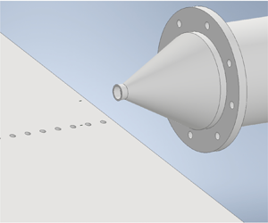
  $0^\circ$, the alignment having being carefully checked using a laser levelling instrument. A scheme of the experimental set-up is given in figure 1.

Figure 1. Sketch of the experimental set-up. Here,  $\xi$ denotes the streamwise separation between the two consecutive pressure transducers.
2.1. Measurement techniques
The wall pressure fluctuations are measured using a pair of miniaturized pressure transducers (Kulite-Mic190M) able to acquire both fluctuating and mean pressure fields and installed in a series of holes manufactured into the plate pressure side. The sensitive diameter is of approximately 3.3 mm, the size of the sensitive surface being small enough not to affect the measured spectra in the range of frequency of interest. The pressure transducers have a sensing diameter that fits the wall pressure taps and a frequency response up to 100 kHz, the unused holes were covered with tape to avoid any vortex shedding effect and cavity resonance. Data were acquired by setting the cutoff filter of the Kulite signal conditioner at 70 kHz and the sampling frequency at 200 kHz, accordingly to the Nyquist–Shannon theorem. Measurements were performed exploring different streamwise positions from  $x/D=1$ up to $x/D=10$ and a schematic view of the transducers positioning is also given in figure 1.
Pointwise velocity measurements were performed using a Pitot probe with the scope of highlighting the modification of the jet flow field due to the presence of the plate. The Pitot tube has been installed on a Thorlabs 2 axis traverse system and moved in an axial direction by step of one nozzle exhaust diameter up to  $x/D=10$, whilst in the radial direction the entire jet plume has been spanned by moving the probe by step of $1/6D$.
In order to provide an overall qualitative picture of the flow behaviour at the different flow regimes and different jet-plate distances, flow visualizations were performed by the application of the BOS technique.
The principles of such a non-intrusive technique, providing an estimation of the density gradient integrated along the optical path, have been extensively described in the past (Richard & Raffel Reference Richard and Raffel2001; Gojani, Kamishi & Obayashi Reference Gojani, Kamishi and Obayashi2013; Raffel Reference Raffel2015), and its applicability in the study of free jets (Clem, Zaman & Fagan Reference Clem, Zaman and Fagan2012; Clem, Brown & Fagan Reference Clem, Brown and Fagan2013) and jet-plate configurations has been assessed in the literature (De Paola et al. Reference De Paola, Di Marco, Meloni and Camussi2019; Camussi et al. Reference Camussi, Ahmad, Meloni, de Paola and Di Marco2022).
The first step of this procedure is the acquisition of a reference image generated by recording a background pattern observed through the air at rest. Thereafter, an additional exposure through the flow under investigation leads to a local displacement of the background pattern. The resulting images of both exposures can now be evaluated by correlation methods. Existing algorithms, developed and optimized for particle image velocimetry (PIV), can be used to determine the displacement of patterns at multiple locations throughout the image. In the present study, a structured background pattern was created in Matlab ambient by generating a  $2000\times 2000$ size matrix of random numbers whose elements are normally distributed and then printed out as a binary image of white dots. The size of the recorded dots is kept at approximately 2–3 pixels as required by the technique in order to obtain a reliable solution. The CCD camera used for the measurements is a LaVision SX 4M with a resolution of $2360\times 1776$ pixels and equipped with a Nikon lens characterised by a focal length of 50 mm. The recording frequency was set to 10 Hz. The pattern was uniformly back illuminated by a white LED screen. To determine the image displacements a PIV cross-correlation algorithm was applied using the Davis software provided by LaVision. The interrogation window was set at a constant size corresponding to $16\times 16$ pixels with a 50 % overlap. Tests were performed by placing the camera and the back-illuminated pattern at the same distance from the nozzle axis as shown in figure 2. For each case, 50 images were acquired and ensemble averaged providing a mean pixel displacement on a grey scale that represents the dimension proportional to mean density gradient fields integrated over the line of sight. It has been checked that the related standard deviation ensured sufficient statistical accuracy for the estimation of the mean values.

Figure 2. Flow visualization experimental set-up.
3. Flow qualification
3.1. Velocity measurements
The mean velocity profiles in the radial and axial directions obtained by the Pitot measurements are reported in figure 3, comparing the isolated case with two different positions of the plate. The local mean velocity is reported in terms of the Mach number and is normalised by the Mach measured at the nozzle exhaust. The curves reported refer to the design conditions but similar results are obtained for the other NPRs and are not reported here for brevity.

Figure 3. Normalised velocity profiles for various jet-plate configurations. (a) Axial evolution at  $y/D=0$. (b) Radial profiles at $x/D=8$.
In figure 3(a) a relevant difference in the axial evolution of the mean velocity is seen in installed configurations compared with the isolated case at large  $x/D$. This is hypothesized as an effect of a local acceleration ascribed to the restricted development of the jet, due to the presence of the plate. This effect was expected considering previous results in the subsonic flow regime (Meloni et al. Reference Meloni, Di Marco, Mancinelli and Camussi2019; Proenca, Lawrence & Self Reference Proenca, Lawrence and Self2019). The radial installed velocity profiles reported in figure 3(b) show a higher jet velocity in the lower shear layer (i.e. close to the plate surface) compared with the isolated case, while installed and isolated jet mean velocity curves collapse well at positive $y/D$ (opposite to the plate). This is observed more intensely at $H/D=0.75$ because of the earlier impact of the jet shear layer over the plate surface. To sum up, as for the subsonic case, the plate restricts the amount of flow entrainment causing a Coanda effect (Proenca et al. Reference Proenca, Lawrence and Self2019).
3.2. Flow visualization
Flow visualizations obtained with the BOS technique provide an overall estimation of the influence of the plate on the shock cell train. Figure 4 illustrates the results obtained in over-expanded (figure 4a,c) and under-expanded (figure 4b,d) conditions. The figures show the trend of the axial component of the displacement vector, which better reveals the shock cell characteristics.

Figure 4. Flow visualizations at different flow velocities and different plate locations. Results are shown for (a)  $H/D=2$ and ${\rm NPR}=2.1$, (b) $H/D=2$ and ${\rm NPR}=2.6$, (c) $H/D=0.75$ and ${\rm NPR}=2.1$, (d) $H/D=0.75$ and ${\rm NPR}=2.6$.
According to the literature (Ben-Dor Reference Ben-Dor2007; Arun Kumar & Rajesh Reference Arun Kumar and Rajesh2017), the cell pattern is significantly modified when moving from over-expanded to under-expanded conditions. As the NPR is raised, the shock cell train exhibits an increasingly pronounced shape and intensity. Also the length of the shock cells changes and increases when the pressure ratio is incremented (André, Castelain & Bailly Reference André, Castelain and Bailly2013). As expected, this length variation is strongly related to the structure of the shock wave reflection. In the over-expanded regime the reflected shock wave does not produce an equal deflection, and the subsequent shock occurs in a closer position than in the under-expanded case (Hadjadj, Kudryavtsev & Ivanov Reference Hadjadj, Kudryavtsev and Ivanov2004; Matsuo et al. Reference Matsuo, Setoguchi, Nagao, Alam and Kim2011). Figure 5 shows the pixel displacement trends along the jet axis ( $y/D=0$) normalised with respect to its mean value in the case of over-expansion (figure 5a) and under-expansion (figure 5b), respectively. For all the NPR values, the effect of the plate is not significantly relevant. More specifically, immediately in the downstream of the jet, the shock cell length only slightly differs between the two configurations while, for increasing $x/D$, the separation between one cell and another remains mostly identical, as illustrated in figure 4 and highlighted in figure 5. It is possible to notice an acceleration of the flow due to the presence of the plate that results in a small delay of the shock cell at the nozzle exit for small $H/D$, which tends to disappear further along the axis. The proximity of the surface increases the intensity of the shocks, leading, in the over-expanded case, to a larger number of shock cells (figure 5a) visible at large $x/D$.

Figure 5. Axial evolution of the pixel displacement at different flow velocities and different plate locations; (a)  ${\rm NPR}=2.1$, (b) ${\rm NPR}=2.6$.
4. Multivariate statistics
An overall picture of the fluctuating wall pressure load is presented through the overall sound pressure level (OASPL), defined as
 \begin{equation} \mathrm{OASPL}=10 \log_{10} \left(\frac{p^{\prime 2}}{P_{{ref}}^2}\right), \end{equation}
where  $P_{{ref}}$ is the reference pressure in air (equal to $20\,\mathrm {\mu }$Pa). Since the lowest frequency acoustic energy, below the anechoic limit of the chamber (i.e. $f < 400\,{\rm Hz}$), contains unwanted reflections and the highest frequency energy contains non-physical background noise, $p'^2$ is computed via integration of the power spectral density (PSD) over a frequency range (Meloni et al. Reference Meloni, Proença, Lawrence and Camussi2021)
 \begin{equation} p'^2= \int_{f_1}^{f_2} \mathrm{PSD}(f)\, {\rm d}f, \end{equation}
where  $f_1$ is 400 Hz and $f_2$ is 20 kHz. The OASPL analysis is reported in figure 6. Different OASPL trends and amplitudes were detected by varying the plate position, due to the different jet-plate grazing. Figure 6(a) reports the OASPL axial evolutions for the over-expanded case showing a quasi-constant trend at $H/D=0.75$ with a maximum at $x/D=3$, and a non-monotonic evolution at $H/D=2$ where the OASPL reaches the maximum where the jet flow impacts the plate ( $x/D=7$) (Camussi et al. Reference Camussi, Ahmad, Meloni, de Paola and Di Marco2022). The OASPL decreasing observed at $H/D=0.75$, especially in the under-expanded case, can be ascribed to the flow development over the plate surface. The authors observed a constant difference (of approximately 10 dB) in terms of OASPL between the two plate locations at the higher axial location ( $x/D>8$). Nevertheless, considering the under-expanded case (see figure 6b), the OASPL axial evolution remains similar to the over-expanded case when the plate is located at $H/D=2$, whereas when reducing the plate location a bump ascribed to the presence of screech noise is observed at $x/D<4$. The OASPL variation due to the plate location remains constant, similar to what was observed in figure 6(a) at $x/D>8$.

Figure 6. Axial evolution of the wall pressure OASPL; (a)  ${\rm NPR}=2.1$. (b) ${\rm NPR}=2.6$.
A spectral analysis of the jet-induced wall pressure field has been performed in terms of single-point statistics depicting the fluctuating pressure load in the frequency domain. Sound pressure level (SPL) spectra are evaluated as
 \begin{equation} {\rm SPL}=10 \log_{10} \left(\frac{ \mathrm{PSD} \Delta f_{{ref}}}{P_{{ref}}^2}\right), \end{equation}
where the PSD is evaluated using Welch's method and  $\Delta f_{{ref}}$ is the frequency bandwidth. Recalling the definition of the Strouhal number
 \begin{equation} St=\frac{fD}{U_j}, \end{equation}
with  $f$ the frequency, $D$ the nozzle exhaust diameter and $U_j$ the jet exit velocity, a series of SPL spectra (plotted as a function of $St$) are shown in figure 7.

Figure 7. Wall pressure spectra at different locations and NPRs. Results are shown for (a)  ${\rm NPR}=2.1$ and $x/D=3$, (b) ${\rm NPR}=2.1$ and $x/D=8$, (c) ${\rm NPR}=2.6$ and $x/D=3$, (d) ${\rm NPR}=2.6$ and $x/D=8$.
Figure 7(a,b) reports spectra acquired in the over-expanded jet cases (i.e.  ${\rm NPR}=2.1$). The trends are mostly broadband for both axial positions and plate locations. According to the low supersonic Mach number, only a slight trace of the BBSAN between $St=0.7$ and $St=0.9$ is detected when the plate is at $H/D=2$ (figure 7a). At $H/D=0.75$ (blue line in figure 7a) this contribution is probably buried by the high-frequency hydrodynamic field generated when the jet grazes over the plate surface. A similar behaviour was observed in subsonic cases (Meloni et al. Reference Meloni, Proença, Lawrence and Camussi2021) where the hydrodynamic component due to the flow development over the rigid surface covered the linear acoustic field.
The wall pressure fluctuations spectra in the under-expanded cases (i.e.  ${\rm NPR}=2.6$) are reported in figure 7(c,d). In these flow conditions the spectral bump related to the BBSAN is more evident due to the higher Mach number. The frequency and amplitude of the BBSAN vary because they depend on the axial location of the pressure transducer and on the distance from the jet flow. According to Edgington-Mitchell (Reference Edgington-Mitchell2019), this is related to the reduction of the shock cell length, the decrease of the energy of the shock train and the reduction of the jet convective Mach number.
In the under-expanded flow conditions several peaks in the spectra are detected for both plate positions. Taking into account the adopted Mach number, the NPR and the  $St$ number of the observed dominant peaks, it is possible to assume that they are the traces of the screech tones that are both identified as toroidal modes (A1 or A2, see Edgington-Mitchell Reference Edgington-Mitchell2019; Li et al. Reference Li, Zhang, Hao and He2020). These modes have been characterised extensively for the cases of under-expanded converging nozzles whereas less investigations have been carried out in supersonic conditions achieved by converging–diverging nozzles and in the presence of a flat plate.
Figure 7(c,d) clearly shows that screech signatures appear differently with the variation of the jet-plate distance. The screech amplitude, as expected, is increased by reducing the jet-plate radial distance due to the closer vicinity of the pressure transducers to the jet plume. Furthermore, as observed in figure 7(c), the vicinity of the plate suppresses the mode A2, while the presumed A1 mode persists with two harmonics. This is probably due to the fact that the plate breaks the symmetry of the jet plume partially inhibiting the symmetric modes. On the contrary, at  $H/D=2$ only the fundamental tones are visible but for both modes since the influence of the plate is weaker and the flow remains axisymmetric. The modification of the screech frequency could be ascribed to a slight modification of the degree of expansion of the jet, maybe producing a slight variation of the position of the shock structures, that could be linked to the increase of the mean velocity observed in figure 3.
Moving farther apart in the streamwise direction (see figure 7d), the effect of the screech is reduced because of the increasing axial distance from the zone of the jet plume containing shock cells. The screech harmonics completely disappear in figure 7(d) as a combined effect of the decrease in the amplitude of the tones due to the increasing distance from the noise source and to the polar dependence in the amplitude of the A1 and A2 modes. Indeed, according to the literature (Edgington-Mitchell Reference Edgington-Mitchell2019), these modes have their major directivity upstream of the nozzle exhaust while their contribution reduces moving downstream. It must also be pointed out that at  $x/D=8$ and $H/D=0.75$, the amplitude of the broadband hydrodynamic component increases significantly as an effect of the grazing of the fully turbulent jet flow, which can partially cover the screech peaks.
In summary, the spectral analysis clarifies that the wall pressure spectra overall amplitude and frequency content are strongly influenced by the governing parameters (i.e.  $x/D$, NPR and $H/D$), and a functional dependence could not be recovered through a simple empirical model.
This is further confirmed by the two-point statistics, investigated in the frequency domain by the computation of the spectral coherence function, a quantity that is crucial to be predicted in order to achieve a complete view of the fatigue stress to which the aircraft structure could be subjected (Blake Reference Blake1986). The coherence function has been evaluated as
 \begin{equation} \gamma(\xi, \eta, \omega)=\frac{ | \phi_{p_{1} p_{2}} ( \xi, \eta, \omega)|}{[ \phi_{p_{1}}(\omega) \phi_{p_{2}}(\omega)]^{{1}/{2}}}, \end{equation}
where  $\omega$ is the angular frequency, $\phi _{p_{1}p_{2}}$ is the cross-spectrum, $\phi _{p_{1}}$ and $\phi _{p_{2}}$ are the auto-spectra of two consecutive transducers separated in the streamwise direction by $\xi$ and in the spanwise direction by $\eta$, in present study both separations being fixed to one dimension. It should be noted that in the present experiment the plate is nominally of infinite length and there are no interactions between the plate trailing edge and the jet. Therefore, the wall pressure coherence has been computed only considering transducers aligned in the streamwise direction, as reported in figure 8, at different axial locations and streamwise separations.

Figure 8. Wall pressure streamwise coherence. Results are shown for (a)  ${\rm NPR}=2.1$ and $x/D=2\unicode{x2013}3$, (b) ${\rm NPR}=2.1$ and $x/D=8\unicode{x2013}9$, (c) ${\rm NPR}=2.6$ and $x/D=2\unicode{x2013}3$, (d) ${\rm NPR}=2.6$ and $x/D=8\unicode{x2013}9$.
A broadband coherence is observed in the cases reported in figure 8(a,b) when the plate is close to the jet plume (at  $H/D=0.75$) because of the fully developed flow overflowing the plate surface. On the other hand, for the plate located at $H/D=2$, a series of bumps around $St=1$ emerge, due to the presence of the BBSAN. Figure 8(c,d) reports the coherence functions at ${\rm NPR}=2.6$. As expected, at large NPR the trace of the screech tones is evident mainly at low $x/D$ (plot (c)) where the grazing flow is less relevant than at large $x/D$ (plot (d)). As was observed from the auto-spectra (figure 7), the presence of the plate leads to the modification of the modes frequencies as well an amplification of their amplitude for small $H/D$.
To the extent of the modelling purposes, the approaches usually adopted in the literature (e.g. Corcos Reference Corcos1964; Smol'yakov, Tkachenko & Wood Reference Smol'yakov, Tkachenko and Wood1991) provide an approximation of the wall pressure coherence function through an exponential decay law (see also Rozenberg et al. Reference Rozenberg, Robert and Moreau2012; Meloni et al. Reference Meloni, Di Marco, Mancinelli and Camussi2019). For the present cases, the presence of peaks and bumps related to screech and BBSAN render this approach quite difficult. Examples of possible exponential approximations are given in figure 9 where the coherence is plotted as a function of the normalised frequency usually adopted in the cited models. It is possible to observe that only for the case at  $H/D=0.75$, $x/D=8$ and ${\rm NPR}=2.1$, where the grazing flow dominates the pressure fluctuations, the exponential approximation applies well whereas it is not reliable for the other cases.

Figure 9. Coherences with exponential decay (dashed lines report the exponential decay laws). Results are shown for (a)  $x/D=7\unicode{x2013}8$ and ${\rm NPR}=2.1$, (b) $x/D=2\unicode{x2013}3$ and ${\rm NPR}=2.6$.
This experimental evidence further motivated the adoption of a data-driven modelling approach, capable of handling efficiently the large number of parameters governing the flow physics and able to reproduce the complex behaviour of the spectral quantities.
5. Metamodel assessment
In the framework described in § 4, a possible approach to model the wall pressure loads and predict in the frequency domain both single- and two-point statistics could be provided by a surrogate model built by means of an ANN. The ANN is here exploited as a data-driven nonlinear model aimed at representing the data acquired in the present experimental campaign. The ANN-based models consist of an analytic function completely defined by a small number of parameters, by means of which it is possible to make predictions in domain regions where the true values are not known. In addition, using a surrogate model based on an ANN implies the possibility of no longer handling large databases.
The ANN model consists of a group of information connections made up of artificial neurons: the elementary unit is the perceptron, a mathematical function that accepts several inputs and retrieves a single output. In the feed-forward, fully connected architecture the network is capable of receiving external signals on a layer of processing units (input nodes), each of which is connected with several inner nodes, organized in different layers: each node processes the received signals and transmits the result to subsequent nodes. A schematic representation of a neural network is in figure 10.

Figure 10. Schematic representation of a neural network with four input nodes, two hidden layers (with seven and four nodes, respectively) and two output nodes.
The learning algorithm is addressed through the so-called training with the backpropagation method. The choice of the network topology and the selection of the parameters that regulate the network training represent a serious challenge since they are highly problem dependent. To overcome the issue, a suitable hyperparameters self-tuning coupled with a fully deterministic topology optimization scheme has been used here (for details, see Appendix A) to derive the metamodel.
5.1. Training set and validation set
The data collected by means of the experimental campaign must be converted into an  $N$-dimensional space suitable to the construction of the model. Specifically, for a given $n$ tuple of the radial distance of the plate $H/D$, axial distance $x/D$ and NPR, the database provides two spectra related to the SPL and the coherence $\gamma$. With the aim at modelling simultaneously spectra and coherence values for a given frequency, the following mixed-integer approach has been adopted:
 \begin{equation} \begin{bmatrix} \text{SPL}_i\\ \gamma_i \end{bmatrix} = \boldsymbol{f}\left({H/D},{x/D},\text{NPR},i_\omega\right). \end{equation}
Here  $i_\omega$ is the frequency index; in this view, SPL and $\gamma$ at the $i$th frequency are the output of the single-frequency multi-point (SFMP) model. The rationale underlying the choice of a SFMP model relies, for example, on the possibility of using the network within an optimal design process, where the objective function must be evaluated thousands of times. Since the network can reproduce single- and two-point statistics with a unique function, providing simultaneously SPL and coherence for a given frequency, the complete set of network parameters (weight matrices and bias vectors) have to be loaded only once by the function evaluator. Such a problem can be translated into a network with four input neurons and two output neurons (in addition to a unknown hidden topology) and $M n_\omega$ points ( $M$ being the number of experiments and $n_\omega$ the number of frequencies) are used to build the model. Since a large number of training points could have represented a computational burden, it has been decided to use the bands representation for the spectra. Moreover, to collect only the desired physical phenomena, some bands were cut both at the beginning and at the end of the spectra. Figure 11 shows how the 1/12 octave band approximation is capable of preserving all the relevant physical information related to both the broadband and tonal components, using a relatively small number of bands.

Figure 11. Comparison between the broadband spectra and its bands representation.
It is also worth noting that, as depicted in figure 11, the tonal screech components location is determined with remarkable accuracy.
The data of the experimental campaign are therefore used to create a database consisting of 7884 elements that define the four variables ( $H/D$, $x/D$, NPR and $i_\omega$) with associated two function values (SPL and $\gamma$). The dataset has been randomly shuffled and 5913 elements were used as training set $\mathcal {T}$, whereas 1971 elements were used as validation set $\mathcal {V}$.
5.2. Network architecture and training
The architecture of the model has been found by solving a minimisation problem in the design space defined by the number of layers, the number of neurons per layer and the kind of activation functions. Specifically, the maximum number of hidden layers has been set equal to three, and five activations are used for the tournament (Gaussian, swish, identity, hyperbolic tangent and cardinal sine). Each optimizer iteration consists of training the current network architecture, and is controlled by an exit rule based on the normalised root-mean-squared error (RMSE) on the training set points RMSE $_\mathcal {T}$,
 \begin{equation} \text{RMSE}_\mathcal{T}= \sqrt{\frac{1}{NM}\sum_{i=1}^M\sum_{j=1}^N\left[ \frac{f_j(\boldsymbol{x}_i)-\hat{f}_j(\boldsymbol{x}_i) }{\max(f_j)-\min(f_j)} \right]^2}, \end{equation}
with  $N$ the number of modelled functions, $M$ the size of the training set $\mathcal {T}$, $\hat {f}_j(\boldsymbol {x}_i)$ the predictions and $f_j(\boldsymbol {x}_i)$ the true values (the terms $\max (f_j)$ and $\min (f_j)$ are used to normalise the error value, making it independent of the functions range). In order to avoid burdensome training of underperforming network configurations, suitable early stop criteria, based on the analysis of different performance metrics, are implemented within the optimizer. The validation error RMSE $_\mathcal {V}$ is also analysed in runtime during the training of the current architecture, and is used to stop the training in case of overfitting.
The calculations for the construction of the model were made on a computer equipped with an Intel Xeon CPU E5-2620 v4. Despite being strongly parallelizable, the optimization algorithm used here makes intentional use of a non-parallel implementation to better highlight the relationship between computing cost and desired accuracy.
For the specific problem, the RMSE $_\mathcal {T}$ target accuracy was set equal to $1.25\,\%$ (the convergence of the network response as a function of the target accuracy is presented in Appendix B), and the optimization algorithm reached the convergence value after 147 iterations, as depicted in figure 12.

Figure 12. The RMSE $_\mathcal {T}$ as a function of the number of iterations.
Figure 12 shows that the optimizer is capable of improving the accuracy (with respect to the initial value) by an order of magnitude in a few iterations, while further improvements are achieved at great computational cost – such behaviour is similar to that of some meta-heuristic optimization algorithms. This is further confirmed by figure 13, which reports the computation time as a function of RMSE $_\mathcal {T}$.

Figure 13. Computation time as a function of RMSE $_\mathcal {T}$ (Intel Xeon CPU E5-2620 v4).
The analysis of figure 13 shows that an accuracy of 5 % in terms of RMSE $_\mathcal {T}$ is reached in less than 5 min, whereas the optimizer drops below the $1.5\,\%$ threshold in just over an hour. To reach the RMSE $_\mathcal {T}$ required target accuracy (set equal to 1.25 %), it takes approximately 5 days. The configuration of the model obtained by means of the optimization process described above has the characteristics reported in table 2.
Table 2. The ANN metamodel final configuration.

5.3. Results and discussion
First we have to compare the response of the model in some points belonging to the training set; indeed, the initial requirement of a model is its ability to reproduce known data. To this aim, the model response in terms of spectra and coherence functions for known axial locations and NPRs are analysed; figure 14 shows original data and model predictions.

Figure 14. Comparison between the ANN metamodel response and original data at different locations. (a) The SPL data and model at  $H/D=0.75$, $x/D=4$ and ${\rm NPR}=2.6$. (b) Values of $\gamma$ and the model at $H/D=0.75$, $x/D=4$ and ${\rm NPR}=2.6$. (c) The SPL data and model at $H/D=0.75$, $x/D=8$ and ${\rm NPR}=2.2$. (d) Values of $\gamma$ and the model at $H/D=0.75$, $x/D=8$ and ${\rm NPR}=2.2$. (e) The SPL data and model at $H/D=0.75$, $x/D=3$ and ${\rm NPR}=2.6$. (f) Values of $\gamma$ and the model at $H/D=0.75$, $x/D=3$ and ${\rm NPR}=2.6$.
The analysis of figure 14 highlights that the ANN model is fully capable of describing the overall dynamics of the vector function; in addition, the generalizing property of the neural networks ensures the regularization of some noisy phenomena (especially for the coherences), typical of experimental data despite the post processing (see, e.g. figure 14(b,d,f).
It is worth noting that, as shown in figure 14(a,b), the peak at  $St\approx 0.7$ is not captured by the model at all. Such a lack can be justified by the objective function that drives the optimization algorithm: the root-mean-square error defined by (5.2) is a global error metric that does not take into account the shape of the functions, and the pointwise differences between the data and the model can be highly non-uniform. To overcome the issue, error metrics based on the concept of ‘distance’ between spectra could be useful; for example, the norm in the vector space defined by the difference between spectra is representative of their differences. Therefore, the norm in the $L^p$ space can be used as a metric to be minimised to match the model of the spectra with the available data. Furthermore, since low values of $p$ enhance the contribution of distributed differences and high values of $p$ emphasise local differences, the choice of $p$ can drive the modelling process towards the minimisation of broadband or tonal component differences (low and high values of $p$, respectively); such an approach has been successfully used in both the aircraft conceptual optimal design and the low-noise flight path optimization (Diez & Iemma Reference Diez and Iemma2012; Centracchio, Burghignoli & Iemma Reference Centracchio, Burghignoli and Iemma2021a; Iemma & Centracchio Reference Iemma and Centracchio2022). Tailored objectives based on the $L^p$ norm are currently under analysis for active modelling problems that involve spectra with significant tonal components (preliminary results can be found in Iemma et al. Reference Iemma, Centracchio, Meloni and Camussi2022).
However, the results in figure 14 clearly show that the dynamics of the data can be replaced by the model response, providing the ability to easily extract information from large databases by using an analytical representation of the data.
Since one of the primary goals of the modelling process is to provide predictions in regions of the domain where there are no experiments or simulations, the model is used to predict the behaviour at conditions outside of the measured data set. Figure 15 shows the model response at  $H/D=0.75$ and $x/D=3.5$ for different NPR values.

Figure 15. Model response for test points at  $H/D=0.75$ and $x/D=3.5$; (a) ${\rm NPR}=2.1$. (b) ${\rm NPR}=2.6$.
It is shown that the screech tone starts to appear at  ${\rm NPR}\approx 2.45$, while for lower NPR values, the spectral dynamics is dominated by broadband phenomena; the frequency domain physics as a function of the NPR is in accordance with expectations.
It is worth emphasising that the model response should be associated with a proper quantification of its uncertainty to provide an estimate of the prediction reliability (here, as specified in Appendix A, the spatial correlation is used to derive the uncertainty function). Figure 16 shows the map of the model response, obtained on a structured grid composed of approximately 80 000 prediction points, at  $H/D=0.75$ and $x/D=3.5$ for all the NPRs, with associated uncertainty values.

Figure 16. The ANN model response and uncertainties at  $H/D=0.75$ and $x/D=3.5$. (a) Model response for the SPL at $H/D=0.75$ and $x/D=3.5$. (b) Model response for $\gamma$ at $H/D=0.75$ and $x/D=3.5$. (c) Model uncertainty for the SPL at $H/D=0.75$ and $x/D=3.5$. (d) Model uncertainty for $\gamma$ at $H/D=0.75$ and $x/D=3.5$. (e) Model global uncertainty function at $H/D=0.75$ and $x/D=3.5$.
Results in figure 16(a,b) look consistent with the literature and the physics. The screech tone, as also depicted in figure 15, appears at  ${\rm NPR}\approx 2.45$, in the region where the jet is under-expanded; the maximum amplitude increases with NPR with a slight Strouhal variation. The ANN model uncertainty related to the SPL turns out to be proportional to the amplitude values, as shown in figure 16(c), whereas the analysis of figure 16(d) highlights that the maximum $\gamma$ uncertainty corresponds to the minimum coherence values; the global metamodel uncertainty, reported in figure 16(e), combines the dynamic properties of the uncertainties related to each component of the vector function. Figure 17 depicts the predictions and the model uncertainty at $H/D=0.75$ and $x/D=3.5$.

Figure 17. The ANN model response and uncertainties at  $H/D=0.75$ and ${\rm NPR}=2.55$. (a) Model response for the SPL at $H/D=0.75$ and ${\rm NPR}=2.55$. (b) Model response for $\gamma$ at $H/D=0.75$ and ${\rm NPR}=2.55$. (c) Model uncertainty for the SPL at $H/D=0.75$ and ${\rm NPR}=2.55$. (d) Model uncertainty for $\gamma$ at $H/D=0.75$ and ${\rm NPR}=2.55$. (e) Model global uncertainty function at $H/D=0.75$ and ${\rm NPR}=2.55$.
In figure 17(a,b) are reported the SPL and coherence maps at for different  $x/D$, fixing the NPR at 2.55 and the position of the plate at $H/D=0.75$. Screech tone frequency, as expected, is constant with $x/D$ being independent of the polar location of the pressure transducer. The screech amplitude decreases as the distance from the nozzle increases due to the dissipation of the shock cell train. The analysis of figure 17(b) underlines, as expected, a higher coherence for the screech frequency, and a smooth low-frequency coherence increasing with a few axial locations downstream of the jet impact point over the plate surface (i.e. $x/D\approx 3.5$), due to an increasing hydrodynamic contribution. Figure 17(c,d) confirms what has been said approximately for the previous case. The map in figure 17(c) shows that the highest uncertainty is related to the maximum SPL amplitudes while the areas with low coherence values imply a lower local uncertainty, as depicted in figure 17(d). These effects are mitigated in the global uncertainty function, reported in figure 17(e).
It is lastly worth highlighting that, similarly to all the surrogate models, the ANN-based model built here has strong restrictions on the possibility of extrapolating data outside the domain identified by the training set. Indeed, although theoretically capable of providing a response also in the outer training frontier, it would not be possible to build the uncertainty function; therefore, the values obtained from the model response should be considered unreliable.
6. Conclusion
An experimental study on the wall pressure fluctuations induced over an infinite flat plate by a single stream supersonic jet has been presented. The plate has been placed tangentially to the jet flow, varying its radial position from  $H/D=0.75$ up to $H/D=2$. The analysis includes wall pressure fluctuations acquired in the streamwise direction using a couple of flush-mounted pressure transducers moved from $x/D=1$ up to $x/D=10$. The NPR has been varied from 2.1 (over-expanded condition) up to 2.6 (under-expanded condition) by steps of 0.1.
An aerodynamic survey is performed using a Pitot probe to the extent of providing a general view of the interaction between the jet and plate surface. A local acceleration, in the axial velocity profile, that could be ascribed to the restricted development of the jet is seen within the vicinity of the plate. Radial velocity profiles showed a higher jet velocity in the lower shear layer in the installed case, revealing the trace of a soft Coanda effect.
The qualitative description of the jet flow fields has been achieved using the BOS technique that provides the visualization of the shock cells and highlights the different behaviours typical of the over-expanded and under-expanded conditions. A slight delay of the shock cell position has been observed when the plate is close to the jet as an effect of the flow acceleration caused by the presence of the plate. The close position of the solid boundary surface also increases the shocks intensity.
A global picture of the fluctuating wall pressure load has been given by the computation of the OASPL, whose trend is strongly influenced by the NPR and the trace of the jet-plate grazing.
The spectral analysis showed clearly the screech and BBSAN signatures. Their trace, in terms of frequency content and amplitude, is significantly influenced by the presence of the plate. According to the considered NPRs, the screech tones are observed to be dominated by the so-called A1 and A2 modes, but at low  $H/D$ ( $H/D=0.75$) the A2 mode is suppressed while the A1 mode persists with the related harmonics. It is worth noting that this mode suppression has been observed for the first time in the present paper, and it is suspected to be related to the breaking of the symmetry of the jet flow field caused by the vicinity of the plate. However, further studies are needed to better clarify the physical mechanism responsible for this phenomenon.
The spectral analysis was extended by considering the two-point statistics. A broadband coherence has been observed at  $H/D=0.75$, where the flow is fully developed over the plate. Nevertheless, a series of bumps related to the BBSAN and screech tones were observed, especially at lower $x/D$, in the under-expanded case, making the coherence not easily reproducible through a model. This is evident in particular close to the nozzle exhaust because of the absence of the jet-plate grazing.
To fulfil the modelling issue, a metamodel based on the ANN approach has been proposed in order to provide a single model capable of predicting both the auto- and cross-spectra. A fully deterministic architecture optimization algorithm has been used to derive the ANN topology and the activation functions combination; the algorithm is coupled with a suitable self-tuning scheme to select the network training parameters. Results show an excellent agreement between the modelled single- and two-point statistics and the original data. As expected, the accuracy of the prediction depends on the number of iterations; in the application presented here, a training set error less than 1.25 % (with a validation error of approximately  $3\,\%$) has been achieved with 147 optimization steps. The model response is capable of correctly reproducing the dynamics of the data, and the predicted values are in accordance with the expected physics. The intensity of the screech is observed depending on the probe position and on the NPR, whereas the screech frequency does not have a polar dependency. Thus, the ANN metamodelling has been demonstrated to be a viable strategy to provide a representative prediction of the jet-induced wall pressure fluctuation in the frequency domain.
Funding
This work has been supported by the European Union's Horizon 2020 research and innovation program under project ENODISE (enabling optimized disruptive airframe-propulsion integration concepts), grant agreement no. 860103.
Declaration of interests
The authors report no conflict of interest.
Appendix A. Active metamodelling using neural networks
Let us consider a fully connected multilayer structure composed of  $L=Q+2$ layers, i.e. the input layer (with $N_i$ input neurons), $\boldsymbol {N_h} = (N_{h_1},\ldots,N_{h_Q})$ hidden neurons organized in $Q$ hidden layers and the output layer (composed of $N_o$ output neurons); the input–output functional relation for each layer can be written as
 \begin{equation} \boldsymbol{a}_l = \boldsymbol{f}_l \left( \boldsymbol{\mathsf{W}}_{l\text{-}1} \boldsymbol{a}_{l\text{-}1}+\boldsymbol{\boldsymbol{b}}_l \right), \end{equation}
with  $\{ \boldsymbol {f}_l \}_{l=2}^{L}$ being the activation functions vector, $\{ \boldsymbol{\mathsf{W}}_l \}_{l=1}^{L\text {-}1}$ the weight matrices and $\{ \boldsymbol {b}_l \}_{l=2}^{L}$ the bias vector. Using the notation of (A1), the inputs $\boldsymbol {x} \equiv \boldsymbol {a}_1$ and the outputs $\boldsymbol {y} \equiv \boldsymbol {a}_L$. The selection of weight matrices and bias vectors (both initialised with random numbers) is performed here with the well-known backpropagation training technique. Such a method involves the minimisation of the cost function
 \begin{equation} C_t = \frac{1}{2}\sum_{i=1}^R \left( \boldsymbol{d}_i- \boldsymbol{y}_{i,t}\right)^2 \end{equation}
for a prescribed number of epochs  $T$. In (A2), $R$ is the number of training set patterns, $\boldsymbol {d}_i$ is the desired output vector and $\boldsymbol {y}_{i,t}$ the network output at the $t$th epoch, both related to the $i$th training pattern. The gradient of the cost function $C_t$ is computed as a series of local intermediate components obtained by backpropagating the information flow from the output layer to the input one. Eventually, weights and biases are updated by means of the learning rate $\eta$. As a result of the training process, the network is identified by its parameters $\varTheta = \{ \boldsymbol {f}_l, \boldsymbol{\mathsf{W}}_{l\text {-}1},\boldsymbol {b}_l \}_{l=2}^{L}$, and the network output is such that $\boldsymbol {\hat {y}_{i}}$ is the image of $\boldsymbol {x}_i$.
Usually, the first goal of the designer is to calibrate the model parameters to ensure an efficient network training such as to ensure a reliable response at any point in the domain. Within this context, two classes of parameters can be identified: the training parameters and architectural parameters. The training parameters affect the training dynamics and include the following parameters: the number  $T$ of training epochs, the batch size $B$ (the number of training data that are propagated through the network), the learning rate $\eta$ and the initial values of weights $\boldsymbol{\mathsf{W}}_0$ and biases $\boldsymbol {b}_0$. The architectural parameters include the network topology (in terms of the number of hidden layers $Q$ and nodes per layer) and the activation function vector $\boldsymbol {f}$. It can be easily noted that the training parameters do not characterise the model but influence its construction, and also provide different convergence properties.
A.1. Training parameters
To avoid the commonly used heuristic approach to the selection of the training parameters, that could constitute a huge computational burden, the active metamodelling strategy implemented makes use of suitable self-tuning of the training parameters. Specifically, the number of epochs  $T$ is selected based on an early stopping criterion: the training process exits if the RMSE related to the training ( ${\rm RMSE}_\mathcal {T}$) set satisfies the designer's needs, or in the event that the RMSE related to the validation set ( ${\rm RMSE}_{\mathcal {V}}$) grows up when ${\rm RMSE}_{\mathcal {T}}$ decreases (as might be an indication of the network overfitting). In addition, a dynamic update of the learning rate $\eta$ is included within the algorithm, with the aim of mitigating the effects of the training instabilities: a runtime control detects the dynamics of the loss function and, if necessary, $\eta$ is shrunk to restore a smooth convergence. It is worth noting that, for both $\boldsymbol{\mathsf{W}}_0$ and $\boldsymbol {b}_0$, uniform random deviate distributions of numbers between 0.0 and 1.0 are generated with a fixed seed to ensure the simulations repeatability; afterwards, the Box–Muller transform is applied to make the distributions normally distributed with zero expectation and unit variance.
A.2. Architecture optimization
It is well known that there is no specific scheme to find the optimal network configuration (in terms of activation functions and topology), thus, a recently implemented fully deterministic optimization scheme has been used to derive the metamodel architecture. Here we want to provide a brief overview of how the optimizer works, without going into details (the complete formulation is the subject of a separate work). Each iteration of the optimization algorithm consists of training a network architecture, and such a training is controlled by an exit rule, based on the normalised RMSE on the training set points. Suitable early stop criteria, based on the analysis of different performance metrics (including the overfitting prevision), are implemented to stop the current training if the analysed topology is poor in terms of fitting performance and no improvement is foreseen. The first step of the optimization algorithm is the selection of the hidden layers number (chosen between 1 and the maximum number of layers set by the designer) and layers initialisation. This is done by testing topologies with a few layers filled with many neurons or many layers filled with a few neurons. Subsequently, based on the performance of the networks calculated in the previous step, the neighbouring networks in the design space identified by the layers and neurons per layer are analysed. Lastly, the topologies with the worst performance are collected and mutations are carried out on them (for example, the number of neurons is exchanged between two contiguous layers) in order to explore the domain. Within the optimization, the training of the current topology is preceded by a tournament for the selection of the best combination of hidden and output layers activation function. Despite the fact that such an initial tournament implies an additional computing effort, it has been noted that such a computational cost is recovered by a faster network training, as the activation functions are the best performing for the specific problem. Recently, the automatic batch size selection has been implemented, which further improves training performance.
A.3. Model uncertainty
The uncertainty of the surrogate model is here provided based on the spatial correlation. To this aim, the ANN response is assumed to be the expectation of a posterior stochastic process: the standard deviation related to the process is modelled as
 \begin{equation} \sigma_\mathcal{N}(\boldsymbol{x})= \begin{cases} \left[ {\dfrac {\sum_{j=1}^{N}{\omega_j(\boldsymbol{x})\hat{y}_j}} {\sum_{j=1}^{N}{\omega_j(\boldsymbol{x})}}- \hat{y}(\boldsymbol{x})} \right]^2 & \text{if}\ \Delta_j(\boldsymbol{x})\neq 0 \ \forall j, \\ 0 & \text{if}\ \exists j \vert \Delta_j(\boldsymbol{x})= 0, \end{cases} \end{equation}
with  $\omega _j(\boldsymbol {x})=\Delta _j^{-\alpha }$, where $\Delta =d(\boldsymbol {x},\boldsymbol {x}_j)$ is the Euclidean distance of a generic point $\boldsymbol {x}\in \mathcal {D}$ and $\boldsymbol {x}_i\in \mathcal {T}$, and $\alpha$ is a parameter to control the decay law of the influence of distant points. Equation (A3) ensures that the variance of the process equals zero at the known data. Under the hypothesis of a continuous uniform distribution bounded by $a(\boldsymbol {x})$ and $b(\boldsymbol {x})$, where $-\infty < a(\boldsymbol {x})< b(\boldsymbol {x})<\infty$, with expectation $\hat {y}$ and variance $\sigma ^2_\mathcal {N}(\boldsymbol {x})$, the uncertainty related to the $j$th component of $\boldsymbol {y}$ is defined as
 \begin{equation} u_j(\boldsymbol{x}) = 2\sqrt{3} \sigma_\mathcal{N}(\boldsymbol{x}), \end{equation}
whereas the global uncertainty  $U(\boldsymbol {x})$ is evaluated as the normalised norm on the $\mathbb {R}^{N}$ Euclidean space
 \begin{equation} U(\boldsymbol{x}) = \sqrt{\frac{1}{N}\sum_{j=1}^{N} u^2_j(\boldsymbol{x})} \end{equation}
to account for all the components of the vector function. Equation (A5) can also be used to estimate the locations of the domain where the knowledge about the dynamics of the target response needs to be improved, e.g. with additional experiments or simulations; its definition can be used to assess adaptive sampling schemes.
Appendix B. Model response convergence
To better understand the role of network training on the functions reproduction, we present here the model of table 2 at different RMSE $_\mathcal {T}$. The model convergence as a function of the training epochs is presented in figure 18, in terms of training loss RMSE $_\mathcal {T}$.

Figure 18. The ANN model RMSE $_\mathcal {T}$ as a function of the number of epochs.
The coloured dots in figure 18 represent different epochs of the training, each one with a different accuracy characterised by  $10\,\%$, $5\,\%$, $2.5\,\%$ and $1.25\,\%$ of RMSE $_\mathcal {T}$. The network responses related to such points are depicted in figure 19.

Figure 19. Visualization of the ANN final model with a different training set RMSE. (a) Model response for the SPL at  $H/D=0.75$, $x/D=4$ and ${\rm NPR}=2.6$. (b) Model response for $\gamma$ at $H/D=0.75$, $x/D=4$ and ${\rm NPR}=2.6$.
Figure 19 shows that the behaviour of the network response as a function of the training epochs is such that the broadband trend of the frequency domain phenomena is first matched. Indeed, the global dynamics of both SPL and  $\gamma$ is roughly described with RMSE $_\mathcal {T}=5$ % – at this accuracy there are no screech peaks. As soon as ${\rm RMSE}_{\mathcal {T}}$ halves ( ${\rm RMSE}_{\mathcal {T}}=2.5\,\%$ after approximately 300 training epochs), the main tonal phenomena at $St\approx 0.3$ become evident. In order to also reproduce the secondary tonal phenomena, it is necessary that the error reaches 1.25 %, at the expense of approximately 1500 additional training epochs.


 Open access