


1. Introduction
Feeding cattle to slaughter is a time-dependent process consisting of production and marketing decisions made along a continuum of time in which a multitude of market and production factors continually change. As such, the determinants of profit change over time. For instance, input costs accrue over time (Bondurant et al., Reference Bondurant, MacDonald, Erickson, Brooks, Funston and Bruns2016; Feuz Reference Feuz2002; Greer and Trapp, 1999; Maples et al., Reference Maples, Coatney, Riley, Karisch, Parish and Vann2015; Wilken et al., Reference Wilken, MacDonald, Erickson, Klopfenstein, Schneider, Luebbe and Kachman2015). Second, individual physical attributes such as live weight, dress percentage, carcass weight, yield grade, and marbling score evolve at diminishing returns to days on feed (Bondurant et al. Reference Bondurant, MacDonald, Erickson, Brooks, Funston and Bruns2016; Bruns et al., Reference Bruns, Pritchard and Boggs2004; Rathmann et al., Reference Rathmann, Bernhard, Swingle, Lawrence, Nichols, Yates, Hutcheson, Streeter, Brooks, Miller and Johnson2012; Rossi et al., Reference Rossi, Loerch, Moeller and Schoonmaker2001; Streeter et al., Reference Streeter, Hutcheson, Nichols, Yates, Hodgen, VanderPol and Holland2012; Tatum et al., Reference Tatum, Platter, Bargen and Endsley2012; Van Koevering et al., Reference Van Koevering, Gill, Owens, Dolezal and Strasia1995). Third, for live cash pen average transactions, the agreed upon price is based in part on both party’s perception of the current average carcass value at that point in time (Jones et al., Reference Jones, Schroeder, Mintert and Brazle1992; Radunz Reference Radunz2010). Fourth, for carcass merit transactions on an individual basis, it is entirely the seller’s responsibility to “best” fit heterogeneous cattle to the grid (formula) on which final payment will be subjected. Finally, the output market at any point in time is expected to deviate from long run and seasonal averages (Anderson and Trapp, Reference Anderson and Trapp2000; Bailey and Brorsen Reference Bailey and Brorsen1985; Peel and Meyer Reference Peel and Meyer2002). Together, these dynamic production processes and market forces result in continually moving targets thus creating significant challenges for feeders to optimally market cattle.
While contending with these dynamic forces, cattle feeders typically harvest cattle between 90 and 300 days on feed, depending upon the rate at which the cattle reach some targeted carcass value (USDA, ERS, 2018). Many cattle feeders market cattle based in part on a visual appraisal of 0.40 to 0.50-inch backfat rule (Bondurant et al., Reference Bondurant, MacDonald, Erickson, Brooks, Funston and Bruns2016; Maples et al., Reference Maples, Coatney, Riley, Karisch, Parish and Vann2015; Wilken et al., Reference Wilken, MacDonald, Erickson, Klopfenstein, Schneider, Luebbe and Kachman2015). This rule-of-thumb marketing method is intended to improve profitability by mitigating the risk that carcasses are overly finished resulting in yield grades discounts yet finished enough to improve the likelihood of quality grade premiums. Bondurant et al. (Reference Bondurant, MacDonald, Erickson, Brooks, Funston and Bruns2016) reported the industry average backfat is 0.47 inches. Also, this marketing methodology appears to be acceptable to buyers and quite possibly used in live cash pen average transactions as a condition of offer and acceptance.
To improve economic efficiency, three prolific though not necessarily mutually exclusive veins of economics literature have emerged; i) the consequences and risks of selling on a live or carcass merit basis,Footnote 1 ii) the exogenous factors that determine price/profitability,Footnote 2 and iii) various sorting strategies.Footnote 3 The first vein generally identifies greater but more volatile profits when selling on a carcass merit basis. The second vein typically ranks the most to least factors for producers to focus their attention. The last vein generally finds that selling like subsets of cattle yield greater profits than selling on a whole pen basis. These studies are of great importance for understanding the economic implications of pricing methodology, impacts of input/output market conditions, production efficiencies, and suggestions for reducing heterogeneity within a marketing group to better align them with a pricing method or production technology. However, after committing to a pricing method and/or technology, the last decision will always be when to market a particular set of cattle, which in turn is contingent on evolving production and market conditions.
A growing amount of literature is specifically aimed at improving the market timing decisions of cattle feeders (Bondurant et al., Reference Bondurant, MacDonald, Erickson, Brooks, Funston and Bruns2016; Feuz, Reference Feuz2002; Greer and Trapp, 1999; Maples et al., Reference Maples, Coatney, Riley, Karisch, Parish and Vann2015; Wilken et al., Reference Wilken, MacDonald, Erickson, Klopfenstein, Schneider, Luebbe and Kachman2015) and is the intended contribution of this research. Not surprisingly, market timing has been shown to have significant consequences on the cattle feeder’s profitability. Therefore, a suboptimal marketing timing decision has the potential to significantly offset expected gains from choices of pricing methods, production practices, and management decisions.
To mitigate market timing errors due to the unobservable carcass characteristics, ultrasound and genetic testing have been developed (e.g., Brethour Reference Brethour2000; DeVuyst et al. Reference DeVuyst, Bullinger, Bauer, Berg and Larson2007; Lusk Reference Lusk2007; Lusk et al., Reference Lusk, Little, Williams, Anderson and Mckinley2003; Norwood et al., Reference Norwood, Lusk and Brorsen2004; Thompson et al., Reference Thompson, DeVuyst, Brorsen and Lusk2014). These technologies have yet to be widely adopted by cattle feeders primarily due to cost, though cost minimizing random sampling techniques for genetic testing have been proposed (Thompson et al., Reference Thompson, Brorsen, DeVuyst and Lusk2017). Alternatively, nearly every feeder today has affordable access to a chute scale and radio-frequency identification (RFID) technology from which individual whole-body growth can be tracked.Footnote 4 It is well known in the beef cattle production literature that quality and yield grade carcass characteristics are correlated with live weight via carcass weight (e.g., Bruns et al. Reference Bruns, Pritchard and Boggs2004; Good et al., Reference Good, Dahl, Wearden and Weseli1961; Owens et al., Reference Owens, Gill, Secrist and Coleman1995; Streeter et al., Reference Streeter, Hutcheson, Nichols, Yates, Hodgen, VanderPol and Holland2012). Therefore, cattle feeders may be able to use live weight information to make informed marketing decisions regarding expectations of carcass value.
The objective of this research is to develop and evaluate a profit maximization methodology that utilizes live weight information to predict carcass value. To do so, predictions of individual whole-body growth are incorporated into predictive models of the underlying carcass characteristics to guide optimal market timing decisions based on carcass value. The methodology is a direct extension of the live cash price dynamic profit maximization method developed by Maples et al. (Reference Maples, Coatney, Riley, Karisch, Parish and Vann2015) [hear after referred to as Maples]. By combining the evolution of carcass characteristics with a corresponding grid (formula) pricing structure, a carcass value-adjusted live cash price path is constructed. This approach is necessary for future application because all marketing timing decisions are made while fed cattle are still alive and accounts for seller and buyer visualizations of carcass value over time. A second extension is to the associated market timing and pricing method literature by considering the implications of seasonal live cash price paths which are inherently dependent on the date the cattle are delivered to the feedlot.
The main simulation results developed informed by a data set containing over 4,000 harvested individuals indicate that the average optimal time cattle are on feed is greater than those observed and more so for the carcass value-adjusted method. These results are consistent with the observed increase in live and carcass weights over the past several decades. Additionally, the carcass value-adjusted methodology is expected to significantly improve profitability with respect to the observed 0.50-inch backfat rule and non-value adjusted (NVA) Maples methodologies. The opportunity cost of incorrectly relying on the carcass value-adjusted method when the NVA Maples method is more appropriate is significantly smaller in magnitude and with less volatility across all identified seasonal price paths than vice versa. Finally, it is demonstrated that the results from comparing marketing methodologies are highly sensitive to the assumptions of the relevant price path.
The structure of the manuscript is as follows. First, a literature review of studies that highlight the importance of optimizing days on feed to maximize profits is provided. Second, the general dynamic profit maximization model that guides the development of the profit simulations is defined. Third, the identification of the whole-body growth and subsequent carcass characteristics predictive equations used in simulations is detailed and evaluated for accuracy. Fourth, identification of the live and value-adjust profit maximization simulation models is developed contingent on the available data. Fifth, simulation results are provided and discussed ending with conclusions and implications of the research.
2. Market Timing Literature Review
Greer and Trapp (1999) conducted a serial slaughter study of mixed breeds over four marketing periods (117, 131, 145, and 159 days on feed). The study estimated whole-body growth from observed feed consumption by means of net energy gain requirements (Fox and Black, Reference Fox and Black1977) and probabilities of observing discrete values for yield and quality grade over time. By means of a profit simulation, the days on feed to market all cattle as a group was identified under various live cash and grid premium/discount transaction prices. The results indicated that the profit maximizing days on feed are strictly greater for live cash than grid transactions. This result is driven by the assumption that discounts for higher yield grades are not applied by buyers in live cash transactions.
Feuz (Reference Feuz2002) simulated the impacts of days fed on profitability based on alternative sets of grid prices under fixed assumptions about whole-body and carcass growth, production costs, and a constant carcass base price. The data consisted of eight different pens of cattle. The analysis found that profitability can be improved for some pens of cattle if fed two weeks longer/shorter depending on whether the grid favors quality/yield characteristics.
Wilken et al. (Reference Wilken, MacDonald, Erickson, Klopfenstein, Schneider, Luebbe and Kachman2015) marketed cattle at three discrete days on feed over the course of five years and seven trials based on when cattle were expected to reach an industry average backfat of 0.47 inches. The results indicated profitability increased with days fed regardless of being sold on a live weight or grid basis, assuming a 63% dress percentage conversion from live to carcass price. Consistent with Feuz (Reference Feuz2002), live weight transaction profits were greater for fewer days on feed, while carcass weight transaction profits were greater for greater days on feed.
Maples developed a dynamic profit maximization methodology from individual estimates of whole-body growth based on a series of five observed live weights, as well as observed daily production costs. They found significant opportunity costs associated with grouping cattle based on a 0.50-inch backfat rule if marketed on an individual live weight basis. Most animals required on average two weeks less than those observed depending on price levels. The opportunity costs on a carcass merit basis, however, could not be estimated from the modeling framework.
Bondurant et al. (Reference Bondurant, MacDonald, Erickson, Brooks, Funston and Bruns2016) found that feeding cattle 44 days longer than the industry’s target of a 0.5-inch backfat resulted in increased profit per head when sold on a grid basis. The increase in carcass weight and quality grade premiums outweighed the increase in yield grade and overweight discounts given average base and grid prices for February 2015. Therefore, market conditions are likely to impact the effectiveness of a 0.5-inch backfat marketing rule.
3. Theoretical Dynamic Profit Model
Maples developed a general dynamic model for the maximization of individual profitability during the feeding process. They assumed that the production technology and feeder cattle purchases are chosen prior to the production period, leaving the marketing date as the final decision based on an optimal stopping rule (Chiang, Reference Chiang1984, pp. 463–464). Whether marketed on a live or carcass merit basis, the decision of when to harvest is made while the animal is still alive and is based in part on the perception of the underlying carcass value. The question of carcass quality, whether estimated or known, also applies to professional buyer willingness to pay.
Using modifications to the notation in Maples without violating the original concepts, the competitive producer’s dynamic profit function for the i th animal is
 $${\pi _i}(t) = {p_i}\left( {{\bf{M}}(t),{V_i}(t)} \right) \cdot {y_i}\left( {t;{{\bf{g}}_i}({{\bf{\gamma }}_i},{{\bf{e}}_T})} \right) - {c_i}\left( {{\bf{w}}(t),{{\bf{x}}_i}(t)} \right) - {F_i}$$
where t is days on feed (DOF). In equation (1), the sales price path ${p_i}$
is a function of time variant market variables
${p_i}$
is a function of time variant market variables ${\bf{M}}(t)$
. For example, live fed cattle cash generally follows seasonal patterns associated with typical changes in supply and demand (Anderson and Trapp, Reference Anderson and Trapp2000). Sales price is also impacted by the expected underlying carcass value,
${\bf{M}}(t)$
. For example, live fed cattle cash generally follows seasonal patterns associated with typical changes in supply and demand (Anderson and Trapp, Reference Anderson and Trapp2000). Sales price is also impacted by the expected underlying carcass value, ${V_i}(t)$
, which is the product of perceived characteristics such as yield and quality grade and their associated market values. The animal’s whole-body growth,
${V_i}(t)$
, which is the product of perceived characteristics such as yield and quality grade and their associated market values. The animal’s whole-body growth, ${y_i}\left( {t;{{\bf{g}}_i}({{\bf{\gamma }}_i},{{\bf{e}}_T})} \right)$
, is a function of time and a set of functional growth parameters,
${y_i}\left( {t;{{\bf{g}}_i}({{\bf{\gamma }}_i},{{\bf{e}}_T})} \right)$
, is a function of time and a set of functional growth parameters, ${{\bf{g}}_i}$
, that identify the shape of the growth function. The growth parameters are in turn a function of intrinsic genetic traits,
${{\bf{g}}_i}$
, that identify the shape of the growth function. The growth parameters are in turn a function of intrinsic genetic traits, ${{\bf{\gamma }}_i}$
, unique to each animal (Lusk Reference Lusk2007), as well as environmental factors,
${{\bf{\gamma }}_i}$
, unique to each animal (Lusk Reference Lusk2007), as well as environmental factors, ${{\bf{e}}_T}$
. Environmental conditions impact the degree of stress experienced until harvested at time T, such as temperature and precipitation. Total variable production cost,
${{\bf{e}}_T}$
. Environmental conditions impact the degree of stress experienced until harvested at time T, such as temperature and precipitation. Total variable production cost, ${c_i}$
, is a function of time-dependent input prices and quantities, for example, price of feed (
${c_i}$
, is a function of time-dependent input prices and quantities, for example, price of feed ( ${w^f}$
), feed consumption (
${w^f}$
), feed consumption ( $x_i^f$
), and daily yardage charges (
$x_i^f$
), and daily yardage charges ( ${w^y}$
) for t days. The cost variable,
${w^y}$
) for t days. The cost variable, ${F_i}$
, is the summation of all other time-independent fixed or sunk costs (i.e., transportation, feeder purchases, and predetermined production strategies).
${F_i}$
, is the summation of all other time-independent fixed or sunk costs (i.e., transportation, feeder purchases, and predetermined production strategies).
Maples detail the requirements for satisfying the necessary and sufficient conditions for optimization (depicted in Maples, equations (2) and (3)). Maples later demonstrate using functional forms of growth that if $p'(t) = 0$
and
$p'(t) = 0$
and ${c_i}^{\prime \prime }(t) = 0$
, then there exists an unrestricted closed-form solution for the optimal marketing day
${c_i}^{\prime \prime }(t) = 0$
, then there exists an unrestricted closed-form solution for the optimal marketing day ${t^*}$
(depicted in Maples, equation (16)). When input prices, output prices, and input quantities are dynamic, multiple local optima may occur but only one will satisfy both conditions globally.
${t^*}$
(depicted in Maples, equation (16)). When input prices, output prices, and input quantities are dynamic, multiple local optima may occur but only one will satisfy both conditions globally.
4. Predicting the Evolution of Carcass Characteristics
This section details the methodology for predicting the evolution of carcass valuation metrics for individual fed cattle based on DOF. The section begins with whole-body growth prediction, ${y_i}\left( {t;{{\bf{g}}_i}} \right)$
, based on feedlot weighing data and is evaluated for accuracy. Next, predictive equations for key carcass value characteristics,
${y_i}\left( {t;{{\bf{g}}_i}} \right)$
, based on feedlot weighing data and is evaluated for accuracy. Next, predictive equations for key carcass value characteristics, ${V_i}(t)$
, based on whole-body growth and serial slaughter literature are detailed.Footnote
5
Finally, the predicted carcass characteristics are compared to those observed from harvest data for accuracy.
${V_i}(t)$
, based on whole-body growth and serial slaughter literature are detailed.Footnote
5
Finally, the predicted carcass characteristics are compared to those observed from harvest data for accuracy.
4.1. Animal Growth and Carcass Data and Description
A unique data set is utilized to estimate individual growth functions. Proprietary data from 2003 to 2011 consisting of over 12,000 head of fed cattle originating from 14 states and fed in 18 feedlots was provided by the Tri County Steer Carcass Futurity Cooperative (TCSCF) in Iowa.Footnote
6
The data are restricted to 4,412 head of Angus and Angus cross-bred steers weighing 500–700 pounds at delivery. The restriction is applied to construct a data set of similar types of cattle to the purebred Angus steers studied in Bruns et al. (Reference Bruns, Pritchard and Boggs2004), a serial slaughter study which contributes to the several of carcass characteristics predictive equations discussed later.Footnote
7
Also, choosing similar breed types of cattle provides some semblance of external control for genetics ${{\bf{\gamma }}_i}$
in equation (1). Individual data include four repeated measures of whole-body weights collected at the respective feedlot: delivery, on-test weight (≈30 days to reach full ration), reimplant, and harvest. Individual age information was available to derive the days on feed for each weighing. It should be noted that the observed harvest weights in the data were estimated rather than recorded from scale observations. Estimates were derived by solving for a common live body weight shrink that results in an average dress of 61.5% for each lot of cattle slaughtered. The data also contain individual carcass characteristics collected by the processing plant at harvest to which characteristics predictions will be compared. These data include individual hot carcass weight, backfat cover, rib eye area, yield grade score, and marbling score.
${{\bf{\gamma }}_i}$
in equation (1). Individual data include four repeated measures of whole-body weights collected at the respective feedlot: delivery, on-test weight (≈30 days to reach full ration), reimplant, and harvest. Individual age information was available to derive the days on feed for each weighing. It should be noted that the observed harvest weights in the data were estimated rather than recorded from scale observations. Estimates were derived by solving for a common live body weight shrink that results in an average dress of 61.5% for each lot of cattle slaughtered. The data also contain individual carcass characteristics collected by the processing plant at harvest to which characteristics predictions will be compared. These data include individual hot carcass weight, backfat cover, rib eye area, yield grade score, and marbling score.
4.2. Live Weight Growth Prediction
Whole-body weight ( ${y_i}$
) is referred to in Maples as live weight (LW). The methodology for estimating the growth in individual LW is as follows. Maples provide an extensive literature review of nonlinear live growth estimation. They estimated two plausible nonlinear live animal growth functions from data collected on fed cattle of Mississippi origin. The first is the Verhulst life cycle logistic growth model which is reliant on age verification for its time variable. The second is a delivery weight adjusted exponential growth model which relies only on DOF for its time variable. Though a moderate improvement in accuracy was observed for the Verhulst model, a large portion of the cattle delivered to feedlots are purchased at auction or intermediaries and are thus not age verified. Because of its wider applicability with only a minor loss in predictive accuracy, the exponential growth model is utilized in this analysis. The predicted LW for each individual animal (i) at DOF
${y_i}$
) is referred to in Maples as live weight (LW). The methodology for estimating the growth in individual LW is as follows. Maples provide an extensive literature review of nonlinear live growth estimation. They estimated two plausible nonlinear live animal growth functions from data collected on fed cattle of Mississippi origin. The first is the Verhulst life cycle logistic growth model which is reliant on age verification for its time variable. The second is a delivery weight adjusted exponential growth model which relies only on DOF for its time variable. Though a moderate improvement in accuracy was observed for the Verhulst model, a large portion of the cattle delivered to feedlots are purchased at auction or intermediaries and are thus not age verified. Because of its wider applicability with only a minor loss in predictive accuracy, the exponential growth model is utilized in this analysis. The predicted LW for each individual animal (i) at DOF $t = [0,{\rm{ }}\infty )$
is
$t = [0,{\rm{ }}\infty )$
is
 $$L{W_{it}} = {e^{ - {k_i}t}}({y_{i0}} - {M_i}) + {M_i}$$
where ${k_i}$
is the intrinsic growth efficiency parameter,
${k_i}$
is the intrinsic growth efficiency parameter, ${y_{i0}}$
is the feedlot delivery weight at
${y_{i0}}$
is the feedlot delivery weight at $t = 0$
, and
$t = 0$
, and ${M_i}$
is the maturity weight parameter that is asymptotically approached as DOF
${M_i}$
is the maturity weight parameter that is asymptotically approached as DOF $t \to \infty $
. The corresponding four percent shrunk live weight used later to estimate carcass characteristics growth is
$t \to \infty $
. The corresponding four percent shrunk live weight used later to estimate carcass characteristics growth is
 $$SL{W_{it}} = 0.96(L{W_{it}})$$
A four percent shrink is commonly used in beef cattle production science literature (Bruns et al., Reference Bruns, Pritchard and Boggs2004). It can be shown that like $L{W_{it}}$
,
$L{W_{it}}$
, $SL{W_{it}}$
is strictly concave and thus exhibits decreasing returns to DOF. Streeter et al. (Reference Streeter, Hutcheson, Nichols, Yates, Hodgen, VanderPol and Holland2012) summarize eight large pen serial slaughter studies conducted between 2007 and 2012 that find decreasing returns to DOF from quadratic regressions.
$SL{W_{it}}$
is strictly concave and thus exhibits decreasing returns to DOF. Streeter et al. (Reference Streeter, Hutcheson, Nichols, Yates, Hodgen, VanderPol and Holland2012) summarize eight large pen serial slaughter studies conducted between 2007 and 2012 that find decreasing returns to DOF from quadratic regressions.
Following Maples, individual growth parameters, ( ${{\bf{g}}_i}$
),
${{\bf{g}}_i}$
), ${k_i}$
and
${k_i}$
and ${M_i}$
are estimated using nonlinear least squares (Lopez et al., Reference Lopez, France, Gerrits, Dhanoa, Humphries and Dijkstral2000). The Gauss-Newton grid search estimates the starting values followed by a Marquardt gradient search to minimize the sum of squared errors (Marquardt, Reference Marquardt1963). For hypothesis testing, the primary assumptions of this estimation procedure are that model errors are mean zero, homoscedastic, and uncorrelated. No error diagnostics are conducted as the only aim of estimation in this application is the predictive qualities of the model specification. During estimation, individual maturity weight parameters are constrained to
${M_i}$
are estimated using nonlinear least squares (Lopez et al., Reference Lopez, France, Gerrits, Dhanoa, Humphries and Dijkstral2000). The Gauss-Newton grid search estimates the starting values followed by a Marquardt gradient search to minimize the sum of squared errors (Marquardt, Reference Marquardt1963). For hypothesis testing, the primary assumptions of this estimation procedure are that model errors are mean zero, homoscedastic, and uncorrelated. No error diagnostics are conducted as the only aim of estimation in this application is the predictive qualities of the model specification. During estimation, individual maturity weight parameters are constrained to ${M_i} \in [1200,{\rm{ }}1800]$
pounds. This strategy eliminates wildly high or low estimates, while providing some flexibility around the mean maturity weights for feedlot steers of 1,641 pounds found by Owens et al. (Reference Owens, Gill, Secrist and Coleman1995). The lower bound is more relaxed relative to the mean to accommodate extremely poor performing cattle due to sickness, poor genetics, or severe environmental conditions.
${M_i} \in [1200,{\rm{ }}1800]$
pounds. This strategy eliminates wildly high or low estimates, while providing some flexibility around the mean maturity weights for feedlot steers of 1,641 pounds found by Owens et al. (Reference Owens, Gill, Secrist and Coleman1995). The lower bound is more relaxed relative to the mean to accommodate extremely poor performing cattle due to sickness, poor genetics, or severe environmental conditions.
4.2.1. Live Weight Prediction Evaluation
Descriptive statistics for LW at each weighing’s average interval length are provided in Table 1. The average delivery weight was 610.65 pounds at 289 days of age, with age ranging from 145 to 803 days. This indicates that the cattle are likely from various phases in the feeder cattle supply chain, from cow/calf weaning through stocker and preconditioning. The average weighing interval post-delivery was approximately 34, 85, and 173 DOF. The average slaughter weight was 1,176.46 pounds. The average age of slaughtered animals was 463 days, with a maximum age of 936 days indicating that most cattle were not old enough to result in over maturity discounts (Tatum, Reference Tatum2012).
Table 1. Summary statistics – live weights and age (N = 4,412)
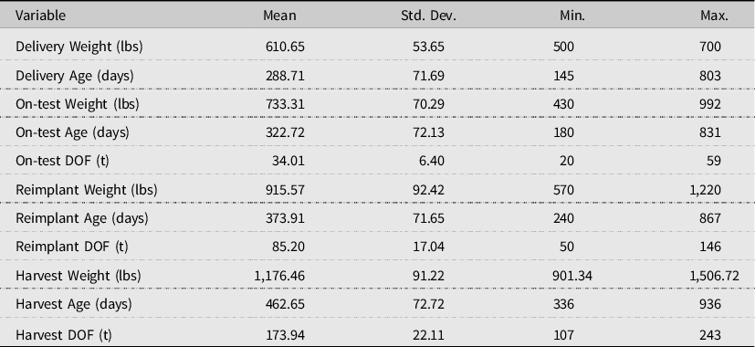
Table 2 provides summary statistics for the estimated growth functions. The average estimated model mean square error is 916.05, as compared to Maples of 1,546.33. The smaller average mean square error is likely due to a narrower weight class and breed type of cattle. The results indicate that harvest weight is underpredicted relative to TCSCF estimates on average by 17.76 pounds, a 1.51% error as compared to Maples of 1.29% error. Overall, both the current estimates and Maples overpredict on-test and reimplant weights and underpredict harvest weight. The estimated average maturity weight is 1,699.39, which is 3.53% greater than predicted by Owens et al. (Reference Owens, Gill, Secrist and Coleman1995). By day 365, the average estimated live weight of the cattle in the study is 1,437.19 pounds, with a corresponding shrunk live weight of 1,379.7 pounds. Because carcass characteristics in the following section are related to LW, diminishing marginal returns to DOF of equation (3) is expected to influence those equations as well.
Table 2. Summary statistics: individual live weight growth estimates (N = 4,412)
Notes: Error = Predicted – Observed.
* Root-mean-square-error.
4.3. Carcass Characteristics Growth Prediction
This section lays out the method for predicting the evolution of individual carcass characteristics that are used in part to derive valuation dynamics on a carcass merit basis, ( ${V_i}(t)$
in equation 1). Seven of the 4,412 observations used to estimate individual whole-body growth had missing values for carcass characteristics at harvest. As such, 4,405 observations were utilized to evaluate the predictive qualities of the carcass characteristics equations.
${V_i}(t)$
in equation 1). Seven of the 4,412 observations used to estimate individual whole-body growth had missing values for carcass characteristics at harvest. As such, 4,405 observations were utilized to evaluate the predictive qualities of the carcass characteristics equations.
To begin, individual dressing percentage growth is derived from individual SLW. Once obtained, the evolution of the underlying hot carcass weight is derived. Next, it will be shown how the predictions of hot carcass weight are used in turn to predict backfat cover and ribeye area growth, both of which are important metrics for predicting USDA yield grade score. Based on the predicted evolution of hot carcass weight, predictions of marbling score are used to in turn derive discrete USDA quality grades.
4.3.1. Dressing Percentage
Bruns et al. (Reference Bruns, Pritchard and Boggs2004) estimated the relationship between dressing percentage (DP) and hot carcass weight (HCW). However, they report HCW and SLW in kilograms while the growth function in equations (2) and (3) is in pounds. The conversion of the DP equation into pounds is provided in Appendix section A.1 and the resulting equation depicted in (a.2) is
 $$D{P_{it}} = 0.4291 + 0.000185(SL{W_{it}}).$$
Because equation (4) is linear in SLW, the DP is strictly concave and exhibits diminishing marginal returns to DOF as does LW.
The mean prediction for the population of cattle analyzed equals 63% at 161 DOF, which is an important valuation benchmark discussed in more detail in the profit modeling section. Bruns et al. (Reference Bruns, Pritchard and Boggs2004) found that on day 250 the cattle dressed on average 65.6%. The current predictions are nearly identical at an average of 65.9%. The predictions from equation (4), however, cannot be compared to those recorded in the TCSCF data due to the estimation of slaughter weights discussed earlier.
4.3.2. Hot Carcass Weight
Bruns et al. (Reference Bruns, Pritchard and Boggs2004) expression of hot carcass weight in the current context is simply
 $$HC{W_{it}} = (D{P_{it}})(SL{W_{it}})$$
Just as LW, SLW, and DP, HCW is strictly concave and exhibits diminishing marginal returns to DOF.
4.3.3. Backfat
The next step is predicting the growth of inches of backfat cover (FC) as measured between the 12th and 13th rib. Though not a value metric, FC is used to predict USDA yield grade, which does impact value, explicitly so in carcass-based transactions. Bruns et al. (Reference Bruns, Pritchard and Boggs2004) estimated centimeters of backfat cover as a function of kilograms of HCW as a function of DOF. The conversion of Bruns et al. (Reference Bruns, Pritchard and Boggs2004) FC equation to pounds is provided in Appendix section A.2. The resulting conversion to inches of FC growth as a function of pounds of HCW is represented in equation (a.4) as
 $$F{C_{it}} = 0.{\rm{214252}} - 0.{\rm{000804}}(HC{W_{it}}) + 0.000002(HCW_{it}^2)$$
It can be shown for the population of cattle analyzed that unlike LW, SLW, DP, and HCW, the mean FC is not strictly concave over DOF $t = [0, 365]$
, but rather slightly cubic. The rate of growth in FC increases at an increasing rate until approximately 175 DOF and then increases at a decreasing rate thereafter. The latter result is due to the influence of the HCW’s diminishing marginal returns. The 0.50-inch backfat target of TCSCF is predicted to occur around 130 DOF, 45 days prior to the average harvest DOF (about 174 days) of the TCSCF cattle (Table 1).
$t = [0, 365]$
, but rather slightly cubic. The rate of growth in FC increases at an increasing rate until approximately 175 DOF and then increases at a decreasing rate thereafter. The latter result is due to the influence of the HCW’s diminishing marginal returns. The 0.50-inch backfat target of TCSCF is predicted to occur around 130 DOF, 45 days prior to the average harvest DOF (about 174 days) of the TCSCF cattle (Table 1).
4.3.4. Ribeye Area
The USDA yield grade equation incorporates the relationship between HCW and square inches of ribeye area (REA) (Lawrence et al., Reference Lawrence, King, Montgomery and Dikeman2001). Using current notation, REA is represented as
 $$RE{A_{it}} = 3.80 + 0.012(HC{W_{it}})$$
By analyzing multi-plant carcass data on 60,625 head of mixed breeds from 1995 to 1997, Lawrence et al. (Reference Lawrence, King, Montgomery and Dikeman2001) found that equation (7) tended to under/overestimate light/heavy carcass and suggested the USDA should adjust the general equation to $RE{A_{it}} = 6.80 + 0.0082(HC{W_{it}})$
. However, given the unknown differences of Angus subtypes and the non-random serial slaughter nature of Lawrence et al. (Reference Lawrence, King, Montgomery and Dikeman2001), the USDA version of REA is retained.Footnote
8
$RE{A_{it}} = 6.80 + 0.0082(HC{W_{it}})$
. However, given the unknown differences of Angus subtypes and the non-random serial slaughter nature of Lawrence et al. (Reference Lawrence, King, Montgomery and Dikeman2001), the USDA version of REA is retained.Footnote
8
4.3.5. Yield Grade
The USDA Yield Grade index (YG) is an explicit value metric in carcass-based transactions and is represented in the current notation as
 $$Y{G_{it}} = 2.50 + 2.50(F{C_{it}}) + 0.20(KPH) + 0.0038(HC{W_{it}}) - 0.32(RE{A_{it}})$$
The percentage of kidney, pelvic, and heart fat (KPH) typically ranges from 2% to 4% and is held constant at an average of 3.50% (Hale et al., Reference Hale, Goodson and Savell2013). Like FC, the increase in the population mean YG over DOF is cubic. The average rate of growth in YG is strictly increasing at an increasing rate until approximately 175 DOF and then increasing at a decreasing rate thereafter. Like FC, the latter result is due to the power of the HCW’s diminishing marginal returns for later DOF. If live and carcass weight changes continue to slow due to maturation, then changes in the underlying carcass characteristics will slow as well.
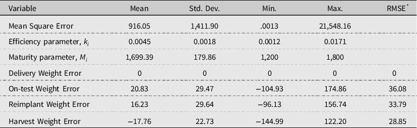
Carcass transactions are based on discrete values of $Y{G_{it}}$
. The predicted distribution of YG categories (1–5) in the population of cattle analyzed is depicted in Figure 1. Initially when the cattle enter the feedlot at DOF zero, 100% of the population is predicted to be a YG 1. By 46 DOF, about half of the population is expected to have evolved from a YG 1 to a YG 2. Once animals have reached 191 DOF, approximately 50% of the population is expected to be YG 3. Yield grade 4 is not present until 146 DOF, while YG 5 are not present until 206 DOF.
$Y{G_{it}}$
. The predicted distribution of YG categories (1–5) in the population of cattle analyzed is depicted in Figure 1. Initially when the cattle enter the feedlot at DOF zero, 100% of the population is predicted to be a YG 1. By 46 DOF, about half of the population is expected to have evolved from a YG 1 to a YG 2. Once animals have reached 191 DOF, approximately 50% of the population is expected to be YG 3. Yield grade 4 is not present until 146 DOF, while YG 5 are not present until 206 DOF.
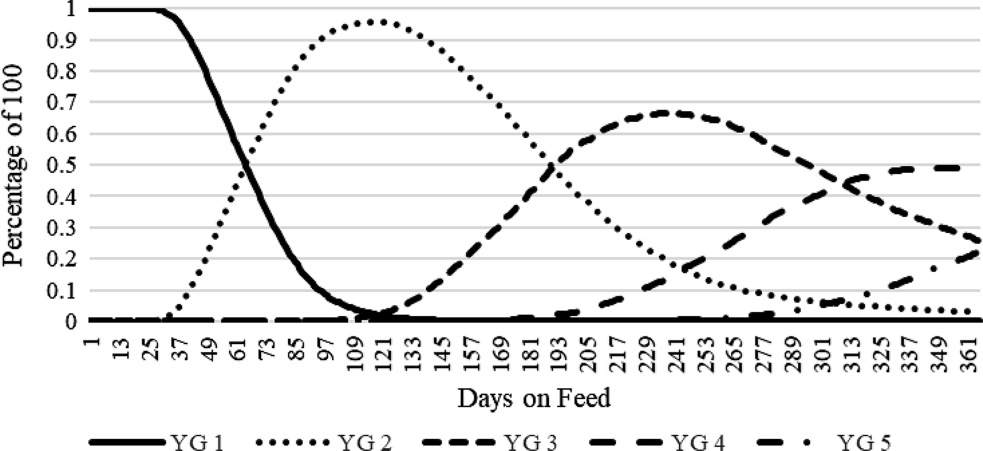
Figure 1. Predicted population yield grade (1–5) distribution dynamics.
4.3.6. Marbling Score and Quality Grade
The final carcass characteristic is marbling score (MS). Like YG, MS directly impacts the value for carcass-based transactions. Bruns et al. (Reference Bruns, Pritchard and Boggs2004) estimated a MS indexing equation. As before, the MS equation is in kilograms of carcass and must also be converted to pounds (see Appendix A.3 for conversion). The resulting MS as a function of pounds of HCW as presented in Appendix Equation (a.6) is
 $$M{S_{it}} = 60.199 + 0.750243(HC{W_{it}})$$
As was the case for HCW, MS is strictly concave and exhibits diminishing marginal returns to DOF.
Carcasses-based transactions are based on discrete values of MS. The numerical value for the $M{S_{it}}$
in equation (9) is converted to a USDA quality grade index (QG), where the break points in are MS 400 = Slight = Select, MS 500 = Small = Choice, MS 600 = Modest = Choice, MS 700 = Moderate = Choice, MS 800 = Slightly Abundant = Prime. The predicted distribution of QG across DOF in the population of cattle analyzed is depicted in Figure 2. The MS equation (9) predicts that 50% of the population enters the feedlot as Select and 50% as standard. At 112 DOF, approximately 50% of the population has converted from Select to Choice. About 40% are expected to achieve Prime by 365 DOF.
$M{S_{it}}$
in equation (9) is converted to a USDA quality grade index (QG), where the break points in are MS 400 = Slight = Select, MS 500 = Small = Choice, MS 600 = Modest = Choice, MS 700 = Moderate = Choice, MS 800 = Slightly Abundant = Prime. The predicted distribution of QG across DOF in the population of cattle analyzed is depicted in Figure 2. The MS equation (9) predicts that 50% of the population enters the feedlot as Select and 50% as standard. At 112 DOF, approximately 50% of the population has converted from Select to Choice. About 40% are expected to achieve Prime by 365 DOF.
Figure 2. Predicted population quality grade distribution dynamics.
4.3.7. Carcass Characteristics Prediction Evaluation
To test the accuracy of the carcass predictions, means difference tests were conducted by comparing those observed at harvest to those predicted from the carcass characteristics equations. The following tests were conducted in using SAS statistical software (SAS/STAT 2016). Before conducting the means difference tests, the Kolmogorov-Smirnov test for normality was performed. The null hypothesis of normal distribution was rejected for all characteristics. Therefore, the Wilcoxon rank sum test was conducted for means tests. Variance tests were conducted by means of the folded form of the F statistic. The resulting means differences tests are provided in Table 3. The results are consistent with those if normality was assumed, and statistically unequal variances are corrected for by the Cochran Test.
Table 3. Individually predicted vs. observed carcass characteristics at harvest (N = 4,405)

Marbling Score (MS) Index: MS < 400 = Standard, MS 400 = Slight = Select, MS 500 = Small = Choice, MS 600 = Modest = Choice, MS 700 = Moderate = Choice, MS 800 = Slightly Abundant = Prime.
Notes:
a Means are significantly different at least α = .01 based on Wilcoxon Ranked Sum test.
Overall, the carcass characteristics equations predict a lighter carcass, more backfat, larger ribeye, lower yield grade, and greater marbling than was observed for the cattle in the data. More specifically, the results indicate that HCW is significantly under-predicted by 14.62 lbs. (2.02%). This result correlates to the under-prediction of live harvest weight and may be somewhat impacted by the assumed four percent live weight shrink which may be more than what is experienced on average. Next, the results indicate that FC is over-predicted by the widest margin of the characteristics at 0.185 (39.30%). The REA is overpredicted by 0.044 square inches (0.36%). On a continuous basis, YG is significantly under-predicted by 0.046 (1.56%) and MS is significantly over-predicted by 51.57 points (9.56%). Though significant differences are found for all carcass attributes, except for backfat, the predictive model errors are relatively small.
5. Dynamic Profit Models
Two types of dynamic profit maximization models are developed from equation (1). The first type of model is NVA as in Maples in that each animal is assumed to receive the same market average live cash price on any given day of sale. Given the underlying carcasses of the live animals evolve heterogeneously by nature, the second type of profit model developed is value adjusted (VA) over time (DOF). This modeling framework is intended to predict the expected evolution of underlying carcass value based on premiums and discounts (grid) applied to individual carcasses characteristics. Both models are simulated assuming a constant output price path as in Maples, as well as average seasonal price movements.
5.1. Price, Grid, and Variable Cost Data and Description
Weekly live steer cash prices spanning the same period as the feedlot data (2003–2011) were collected from the AMS Five Area Weekly Weighted Average Direct Slaughter Cattle report (USDA, AMS, 2019a). Descriptive statistics are reported in Table 4. The market average live cash price is $91.07/cwt. A seasonal price path is constructed by a simple averaging routine of the corresponding weekly live cash prices across the seven years of data (2003–2011).Footnote 9 Figure 3 depicts a constant $91.00/cwt and the seasonal live cash price paths, assuming an October delivery. The discrete (step function) nature of the series is due to weekly negotiated prices apply to all days within a week.
Table 4. Optimal cattle characteristics by marketing method (N = 4,412)
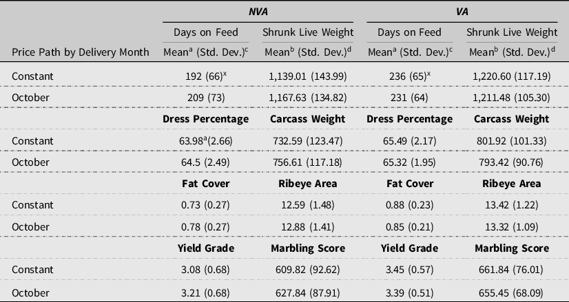
Notes: NVA = Non-value Adjusted Method and VA = Value-adjusted Method.
a, b All paired NVA and VA row means are significantly different at α = .001 based on Wilcoxon Ranked Sum test.
c, d All but
x paired NVA and VA row variances are significantly different at α = .001.
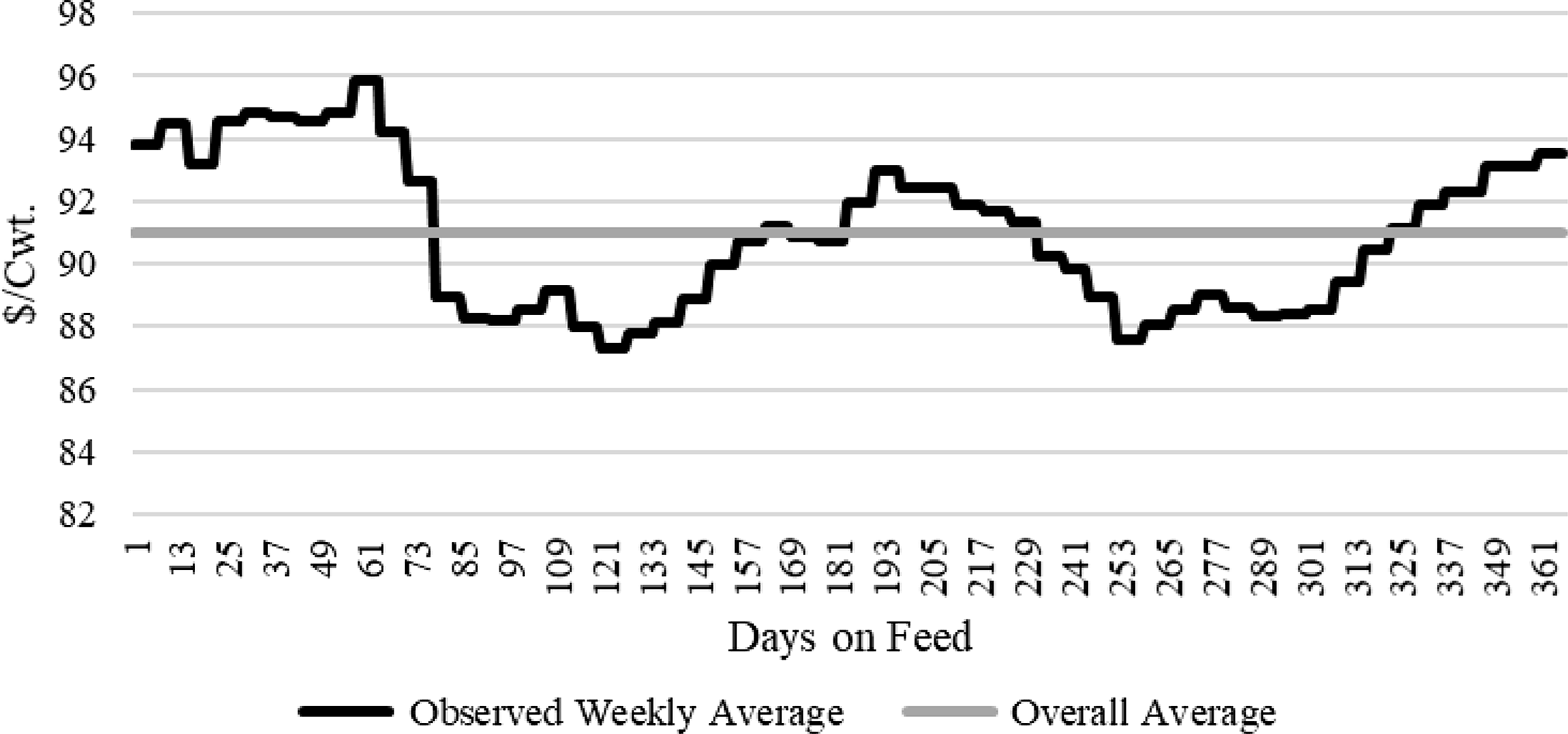
Figure 3. Five area live cash price path – October delivery (USDA, AMS, 2019a).
Weekly steer carcass dress prices were collected from the AMS Five Area Weekly Weighted Average Direct Slaughter Cattle report (USDA, AMS, 2019a). Data are only available starting the week of 10/27/2003. Descriptive statistics are reported in Table 4. The corresponding average carcass dress price is $144.67/cwt. The implied market dress percentage relationship between live cash and dress prices is calculated by dividing the weekly live cash price by its corresponding reported dress price. The average implied dress relationship is 62.98% (approximately 63%). The implied dress percentage will be used to equate carcass prices for the VA model on an NVA live animal basis. Finally, grid prices for slaughter cattle were obtained from the AMS’s Five Area Weekly Weighted Average Direct Slaughter Cattle Steers and Heifers Premiums and Discount report (USDA, AMS, 2019b). Average quality grade, yield grade, and carcass weight premiums and discounts are derived on a carcass weight basis and reported in Table 5.

Though daily production costs may vary across time, the data from TCSCF include only total variable input cost measurements. The inputs that contribute to variable costs of production that accrue over time are feed, micro-ingredients,Footnote 10 yardage,Footnote 11 and interest. Total dry matter feed consumption on an individual basis is estimated by means of the Cornell Net Carbohydrate and Protein system (Tedeschi et al., Reference Tedeschi, Fox and Baker2004).Footnote 12 Given total feed consumed, reported total feed costs are then prorated on an individual basis. Average daily variable costs of production are calculated by dividing the sum of the variable factor costs by the DOF at harvest. The average daily variable factor cost is $1.84/day. Feed contributes roughly 90% to the daily variable production costs.
5.2. Non-Value Adjusted Profit Model
The NVA profit maximization simulation model follows directly from Maples. However, modifications are made to enhance the applicability to real-world transactions. First, buyers derive pay-weights by shrinking the live weight to account for the contents of the digestive tract. Maintaining the assumption of a four percent shrink, $SL{W_{it}}$
represents the pay weight which substitutes for
$SL{W_{it}}$
represents the pay weight which substitutes for $L{W_{it}}$
. Secondly, output price may exhibit seasonal variation.
$L{W_{it}}$
. Secondly, output price may exhibit seasonal variation.
The producer’s NVA profit objective function for each of i animals is
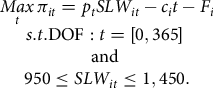 $$\matrix{ {\mathop {Max}\limits_t {\pi _{it}} = {p_t}SL{W_{it}} - {c_i}t - {F_i}} \cr {s.t.{\rm{DOF}}:t = [0,365]\;} \cr {{\rm{and}}\;} \cr {950 \le SL{W_{it}} \le 1,450.} \cr } $$
In equation (10), ${p_t}$
is the weekly average live cash price path and accounts only for market factors,
${p_t}$
is the weekly average live cash price path and accounts only for market factors, ${\bf{M}}(t)$
, from equation (1). Weekly average price is applied to all individuals for each day of a given week as a negotiated live or base price is customarily good for the entire week of delivery.Footnote
13
Regarding seasonal price movements, the relevant simulated price path depends on the month the feeder cattle are delivered to the feedlot. The total variable factor cost term,
${\bf{M}}(t)$
, from equation (1). Weekly average price is applied to all individuals for each day of a given week as a negotiated live or base price is customarily good for the entire week of delivery.Footnote
13
Regarding seasonal price movements, the relevant simulated price path depends on the month the feeder cattle are delivered to the feedlot. The total variable factor cost term, ${c_i}t$
, in equation (10) represents the accrual of daily input variable factor costs. The marginal factor cost is treated as constant rather than dynamic as only total variable factor costs are known in the data. A closed-form solution to equation (10) does not exist with the seasonal prices as depicted in Figure 3. This is due to the discrete jumps in price across weeks. Therefore, optimization of (10) is determined by means of a numerical grid search for the DOF when profit is maximized.
${c_i}t$
, in equation (10) represents the accrual of daily input variable factor costs. The marginal factor cost is treated as constant rather than dynamic as only total variable factor costs are known in the data. A closed-form solution to equation (10) does not exist with the seasonal prices as depicted in Figure 3. This is due to the discrete jumps in price across weeks. Therefore, optimization of (10) is determined by means of a numerical grid search for the DOF when profit is maximized.
The shrunk weight boundaries are chosen assuming a 63-dressing percentage resulting in roughly 600-to-900-pound carcasses.Footnote 14 It is assumed that sellers/buyers of live cattle would at least attempt to trade within the weight restriction to avoid the respective discounted values on a carcass merit basis. The weight restriction, therefore, restricts some market timing solutions that are outside the boundaries.
5.3. Value Adjusted Profit Model
To determine the VA profit for a live animal in the feedlot, live cash prices are adjusted by incorporating expectations of the underlying carcass value as represented by ${V_i}(t)$
in equation (1). The producer’s VA profit objective function is
${V_i}(t)$
in equation (1). The producer’s VA profit objective function is
 $$\mathop {Max}\limits_t {\pi _{it}} = D{P_{it}}\left[ {\rho (t) + {{\bf{C}}_i}(t){\bf{v}}(t)} \right]SL{W_{it}} - {c_i}t - {F_i}$$
The term $D{P_{it}}[{\bullet}]$
is a structural expression of
$D{P_{it}}[{\bullet}]$
is a structural expression of ${p_i}\left( {{\bf{M}}(t),{V_i}(t)} \right)$
in equation (1). The term in brackets [
${p_i}\left( {{\bf{M}}(t),{V_i}(t)} \right)$
in equation (1). The term in brackets [ $\bullet$
] is the expected value of the underlying carcass. Multiplying by
$\bullet$
] is the expected value of the underlying carcass. Multiplying by $D{P_{it}}$
generates the individual’s expected live value equivalent price path. Thought of another way, multiplying
$D{P_{it}}$
generates the individual’s expected live value equivalent price path. Thought of another way, multiplying $D{P_{it}}$
and
$D{P_{it}}$
and $SL{W_i}(t)$
generates the expected carcass weight multiplied by the expected value of the underlying carcass.
$SL{W_i}(t)$
generates the expected carcass weight multiplied by the expected value of the underlying carcass.
The term $\rho (t)$
in equation (11) represents the carcass base (dress) price reported in Table 4. The carcass base price is derived
$\rho (t)$
in equation (11) represents the carcass base (dress) price reported in Table 4. The carcass base price is derived $\rho (t) = p(t)/d(t)$
, where
$\rho (t) = p(t)/d(t)$
, where $d(t)$
is the implied market dress percentage. The base price is associated with a Choice Yield Grade 3 carcass in industry grid (formula)-based transactions. To complete the solution for [
$d(t)$
is the implied market dress percentage. The base price is associated with a Choice Yield Grade 3 carcass in industry grid (formula)-based transactions. To complete the solution for [ $\bullet$
], the base carcass price is adjusted by the net solution from multiplying a 1 X k vector of expected carcass characteristics,
$\bullet$
], the base carcass price is adjusted by the net solution from multiplying a 1 X k vector of expected carcass characteristics, ${{\bf{C}}_i}(t)$
, by a corresponding k X 1 vector of grid premiums/discounts,
${{\bf{C}}_i}(t)$
, by a corresponding k X 1 vector of grid premiums/discounts, ${\bf{v}}(t)$
. Unlike the NVA model in equation (11), the VA model is no longer subject to a range of live harvest weights. This is because the expectations of carcass weight discounts within
${\bf{v}}(t)$
. Unlike the NVA model in equation (11), the VA model is no longer subject to a range of live harvest weights. This is because the expectations of carcass weight discounts within ${\bf{v}}(t)$
are contingent upon the current state of the animal’s HCW growth accounted for in equation (5). A closed-form solution to equation (11) does not exist given discrete jumps in price across weeks in addition to the application of premiums and discounts to discrete carcass valuation metrics. As is the case for the NVA model, optimality is determined by means of a numerical grid search for the maximum profit and respective DOF.
${\bf{v}}(t)$
are contingent upon the current state of the animal’s HCW growth accounted for in equation (5). A closed-form solution to equation (11) does not exist given discrete jumps in price across weeks in addition to the application of premiums and discounts to discrete carcass valuation metrics. As is the case for the NVA model, optimality is determined by means of a numerical grid search for the maximum profit and respective DOF.
5.4. Live Value Equivalent Price Path Series
Expected live value equivalent price path is constructed based on the following parameterization. Though the reported carcass dress price may be used directly for $\rho (t)$
, dividing
$\rho (t)$
, dividing $p(t)$
by the average
$p(t)$
by the average $d(t)$
of approximately 0.63 (Table 5) creates a directly comparable price series between the two models via
$d(t)$
of approximately 0.63 (Table 5) creates a directly comparable price series between the two models via $p(t)$
. Comparing the coefficient of variations in Table 5 shows some
$p(t)$
. Comparing the coefficient of variations in Table 5 shows some ${\bf{v}}(t)$
to be more volatile than live cash prices (i.e., Select, YG 4, and carcass weights). The mean values of
${\bf{v}}(t)$
to be more volatile than live cash prices (i.e., Select, YG 4, and carcass weights). The mean values of ${\bf{v}}(t)$
in Table 5 are utilized to control for the dynamics of carcass characteristics’ supply and demand. This provides a concise comparison of outcomes between the NVA and VA models.
${\bf{v}}(t)$
in Table 5 are utilized to control for the dynamics of carcass characteristics’ supply and demand. This provides a concise comparison of outcomes between the NVA and VA models.
The resulting population’s mean live value equivalent price path is provided in Figure 4, assuming a constant live cash price, $p(t)$
, equal to $91.00/cwt. The price path depicts the evolution in the trade-offs between carcass quality (MS) and cutability (YG). From the onset of the feeding process, the combination of expected discounts from lightweight and standard carcasses and lower dressing percentage result in a lower live value equivalent path relative to live cash price. At 166 DOF, the live value equivalent and cash prices are equivalent. At around this point in DOF, the average animal is expected to reach the base value metrics of 63% dress, YG 3, Choice carcass per equations (4), (8) and (9), respectively.Footnote
15
Beyond 166 DOF, the live value equivalent price path exceeds the live cash price. This is due to
$p(t)$
, equal to $91.00/cwt. The price path depicts the evolution in the trade-offs between carcass quality (MS) and cutability (YG). From the onset of the feeding process, the combination of expected discounts from lightweight and standard carcasses and lower dressing percentage result in a lower live value equivalent path relative to live cash price. At 166 DOF, the live value equivalent and cash prices are equivalent. At around this point in DOF, the average animal is expected to reach the base value metrics of 63% dress, YG 3, Choice carcass per equations (4), (8) and (9), respectively.Footnote
15
Beyond 166 DOF, the live value equivalent price path exceeds the live cash price. This is due to $D{P_{it}}$
adjusting for the added sales value from increasing saleable carcass weight, as well as the increasing frequency of carcass quality premiums outweighing the frequency of discounts primarily from higher yield grades. A maximum mean population value is approximately attained at approximately 229 DOF. However, as DOF increases further, the frequency of heavyweight and YGs 4 and 5 discounts increase, the value path converges back toward the live cash price. These simulated results are consistent with the empirical findings of Schroeder and Graff (Reference Schroeder and Graff2000). Though not presented, the same forces can be seen when applied to each seasonal price path.
$D{P_{it}}$
adjusting for the added sales value from increasing saleable carcass weight, as well as the increasing frequency of carcass quality premiums outweighing the frequency of discounts primarily from higher yield grades. A maximum mean population value is approximately attained at approximately 229 DOF. However, as DOF increases further, the frequency of heavyweight and YGs 4 and 5 discounts increase, the value path converges back toward the live cash price. These simulated results are consistent with the empirical findings of Schroeder and Graff (Reference Schroeder and Graff2000). Though not presented, the same forces can be seen when applied to each seasonal price path.
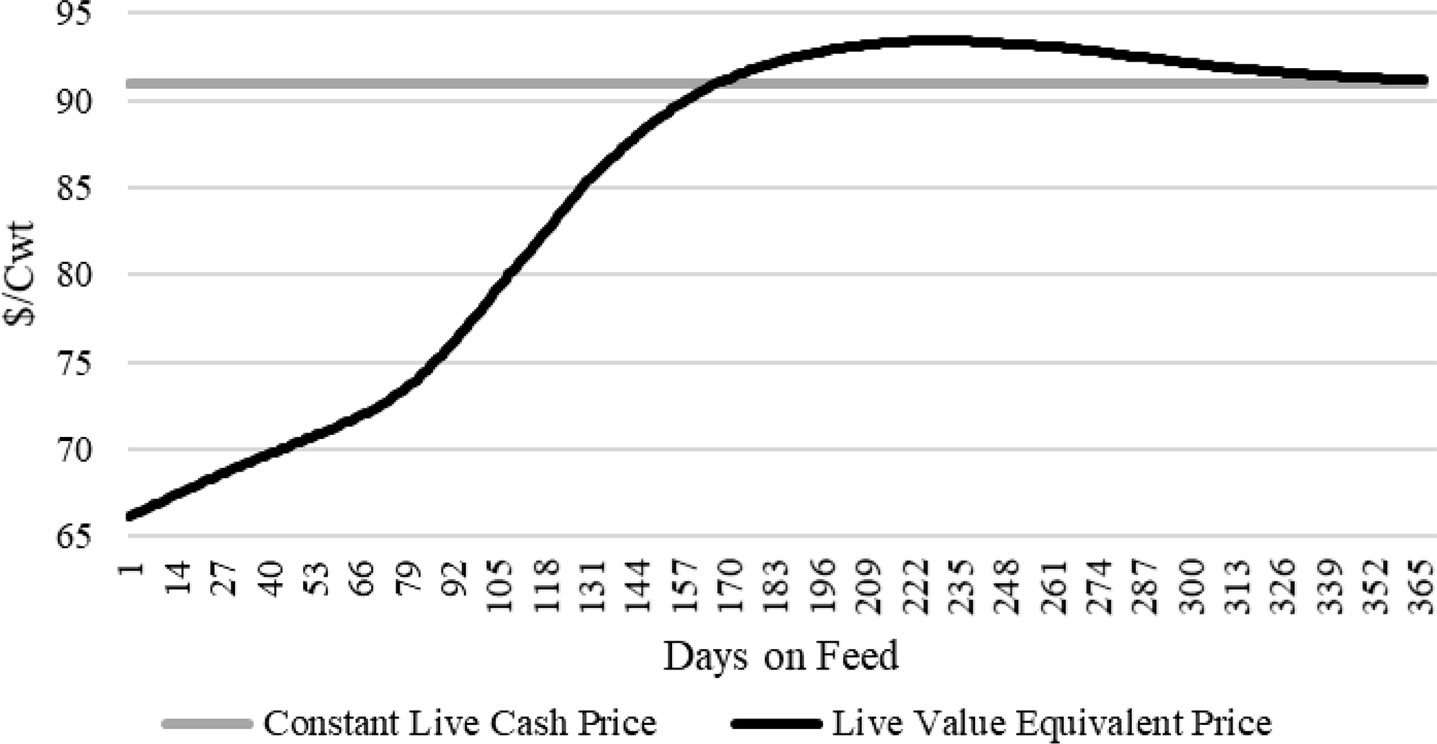
Figure 4. Population mean price and value paths.
6. Profit and Opportunity Cost Results
Predicted profits are compared between marketing methodologies: the end-point carcass marketing approach observed in the data, in which like subgroups of cattle are marketed based primarily on a visual appraisal of attaining 0.5 inches of backfat, and individuals marketed based on NVA and VA dynamic profit maximization. To maintain focus on the additional profits from feeding, the noise in realized profits caused from the contributing factors of ${F_i}$
(i.e., feeder purchases, prorated trucking, pharmaceutical) is not deducted in the profit results. Therefore, all reported profit levels are in returns over total variable factor cost, while marketing method comparisons are in absolute profit differences. Twelve seasonal live cash price path comparisons are conducted between the NVA and VA by assuming cattle are delivered at the beginning of the first full week of each month. The NVA and VA optimal DOFs and expected profits are then compared. The final comparisons are the expected opportunity costs among the three marketing methodologies and across alternative price paths.
${F_i}$
(i.e., feeder purchases, prorated trucking, pharmaceutical) is not deducted in the profit results. Therefore, all reported profit levels are in returns over total variable factor cost, while marketing method comparisons are in absolute profit differences. Twelve seasonal live cash price path comparisons are conducted between the NVA and VA by assuming cattle are delivered at the beginning of the first full week of each month. The NVA and VA optimal DOFs and expected profits are then compared. The final comparisons are the expected opportunity costs among the three marketing methodologies and across alternative price paths.
6.1. Population Mean Dynamic Profit Paths
The NVA and VA profits are first estimated assuming a constant live cash price path of $91.00/cwt. Figure 5 depicts the mean population profit path for each method. These results are on par with a hypothetical pen average marketing strategy. The resulting VA profit path, which follows a pattern like the price paths depicted in Figure 4, illustrates how influential the evolution in carcass valuation is on profitability. Up until 163 DOF, the expected VA profit path is less than NVA. This is due to the higher predicted frequency of discounts for light weight, as well as the frequency of lower-quality grades (Figure 2). However, this negative result is offset to some degree by the higher predicted frequency of premiums for lower yield grades (Figure 1). At 163 DOF, the profit series are equal, again due to the population mean equaling the base dress percentage, yield, and quality grade value metrics. Beyond 163 DOF, the VA profit path is generally greater than NVA, but as observed in the live value equivalent price path (Figure 4), approaches NVA at 365 DOF. This result is due to expectation of DP greater than 63% accounting for the increased value of higher yielding carcass. The maximum VA profit occurs at 208 DOF, while the NVA’s maximum profit occurs at 174 DOF. These differences suggest an incentive to feed cattle longer under expectations of increasing carcass quality and value over the base. After 208 DOF, the VA profit path declines indicating a reduction in profitability due to increases in the expected frequency of discounts for higher YG’s, (Figure 1), and heavy weight carcass discounts. The decline in profit is faster than in the live value equivalent price path (Figure 4) due to the impacts of diminishing returns to DOF in carcass growth (equation 5). Though not presented, the same forces can be seen for each seasonal price path.
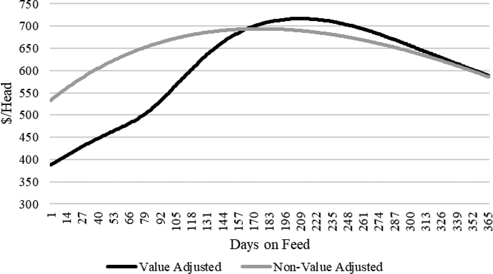
Figure 5. Population mean profits1: constant live cash price path.
6.2. Individual Optimal Profits
Means, standard deviations, and respective paired statistical tests of the optimal DOF and predicted profits between the NVA and VA methods for each price path are reported in Table 6. The results indicate that VA cattle are fed significantly longer than NVA. For the exception of a constant price path and May through July delivery price paths, the NVA DOF are significantly less volatile. The longer feeding can be attributed to the VA model predicting improvements in marbling but selling before suffering yield grade discounts. For most delivery price paths, the reduction in DOF volatility is likely driven by the truncation of cattle into pre-discounted groups. The results also indicate that regardless of price path, the VA method predicts significantly greater, but more volatile, profits than the NVA. Mean profit differences ranged from $25.86/head for August to $48.58/head for March delivery, while volatility differences ranged from 10.51% for March delivery to 28.50% for a constant price path. The mean profit difference results are consistent with the $35.00/head increase in revenue found by Schroeder and Graff (Reference Schroeder and Graff2000), but much less than the two-fold increase in revenue volatility found by the authors.
Table 6. Optimal market timing and profits1 by profit method (N = 4,412)
1Profits reported exclude time independent fixed and sunk costs.
Notes: NVA = Non-value Adjusted Method and VA = Value-adjusted Method.
a, b All paired NVA and VA row means are significantly different at α = .001 based on Wilcoxon Ranked Sum test.
c, d All but
x paired NVA and VA row variances are significantly different at α = .001.
Figure 6 depicts the distribution of DOF on a weekly basis of the observed harvest and each optimal profit model assuming a constant price path. Even with the minimum live weight restrictions, the NVA allows more cattle to be marketed before 100 DOF than observed marketing or suggested by the VA method. The reason being is that both the observed and VA suggested marketing decisions account for under finishing of cattle. A possible reason for the bulk of the VA method shifting cattle to greater DOF relative to those observed is it tended to predict a lower carcass weight and yield grade at harvest (Table 3). This would lead to the belief that YG 4, YG 5, and heavy weight discounts will not occur until later than believed when the cattle were marketed. Given carcass metrics could only be observed once, the validity of the VA belief remains in question. Finally, it is important to note that the smaller observed DOF volatility is not directly comparable to the NVA and VA methods because trucking logistics restrict marketing’s into “like” groups reducing the delivery freedom assumed in the simulations.
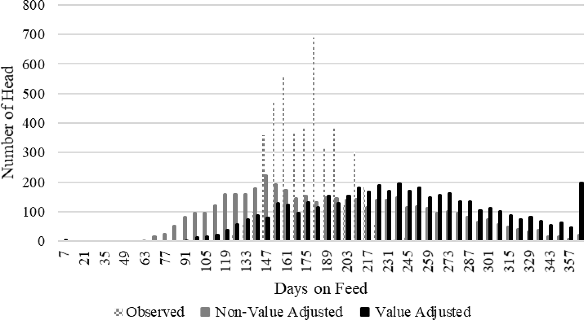
Figure 6. Distribution of days on feed marketed: constant live cash price path.
Figure 7 depicts the impact on the overall distribution of optimal DOF for each profit-based methodology on a weekly basis for the October delivery seasonal price path. The optimal DOF for both methods tends to cluster around peak prices after 163 DOF once the predicted average animal has reached the base value and average dress percentage. However, the VA method tends to spread the optimal DOF between peak periods to take advantage of the expected improvement in carcass value even with weaker prices.
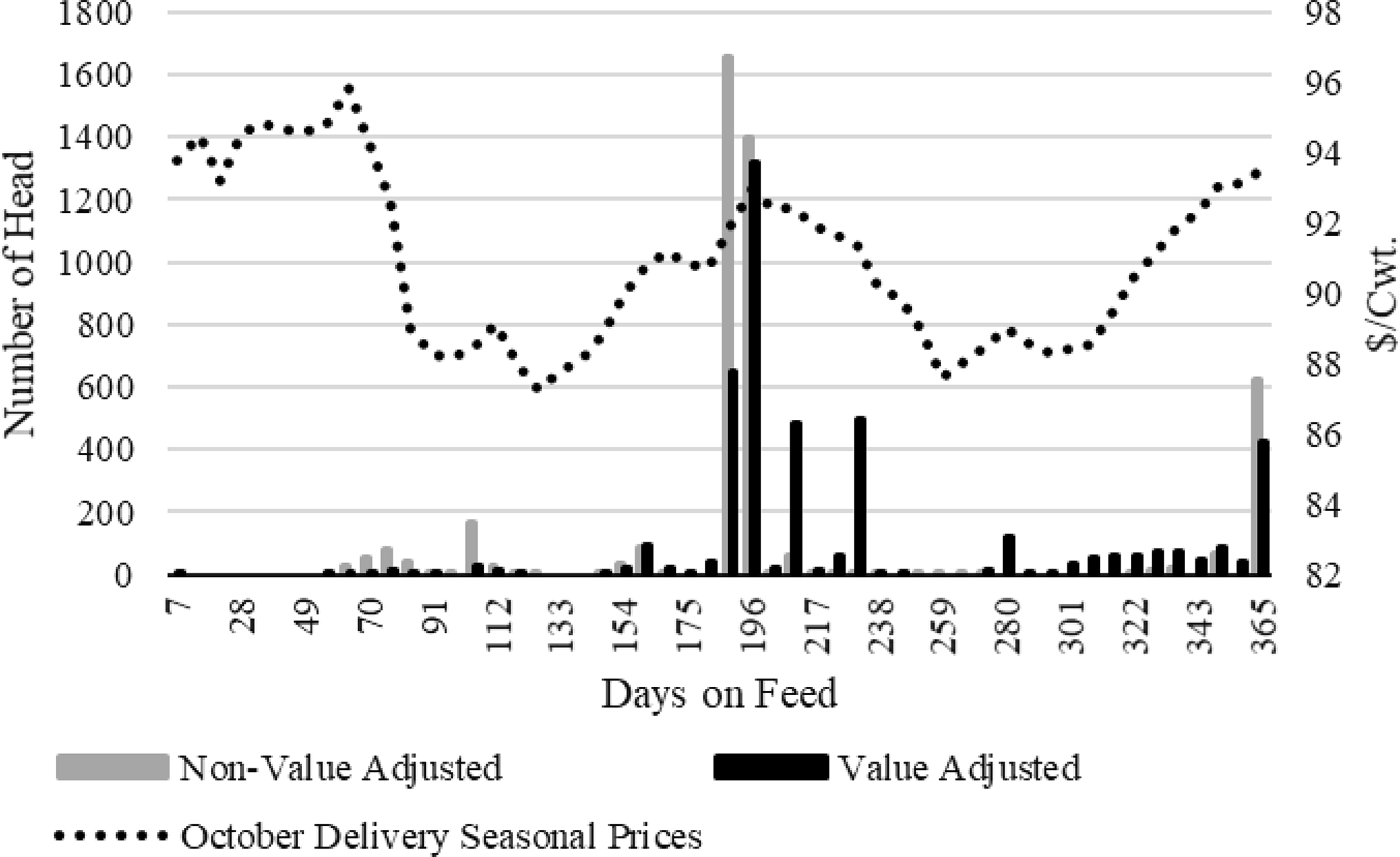
Figure 7. Distribution of days on feed marketed: October delivery seasonal live cash price path.
Table 4 reports the means, standard deviations, and respective paired statistical tests of the predicted cattle characteristics between the NVA and VA methods for the constant and October delivery price paths. Given the VA method tends to feed cattle longer, it is not surprising that the VA method results in significantly greater SLW and by extension increases all predicted carcass attributes (DP, HCW, FC, REA, YG, and MS). As with optimal DOF volatility, carcass attribute volatility shows a significant reduction for the VA as compared to the NVA method, a result that occurs by definition of the methodologies. These results hold for both constant and the October delivery price path as well.
6.3. Opportunity Costs
The marketing method opportunity costs are calculated as
 $${\varepsilon _{i|m}} = {\pi _{i|m}}(t_{i|m}^*) - {\pi _{i|m}}(t_{i| - m}^*)$$
where m is the marketing methodology of interest from which its optimal profits are compared to as if decisions were made by the –m other dynamic profit maximization methodology. Equation 12 is positive/zero when the optimal DOF are unequal/equal.
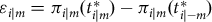
Table 7 reports the opportunity costs of for each methodology and each price path as compared to the observed harvest DOF and with each other. The mean opportunity costs with constant prices of the observed harvested DOF relative to the NVA method is $16.94/head. This result is larger in magnitude than the $5.33–$5.89/head found in Maples for the same weight classes, live price, and similar growth parameter estimates as in this analysis. Maples did not report estimates of optimal DOF or break out observed DOF by weight class from which to establish basic differences. A potential explanation of the difference is that Maples reported higher average daily variable factor costs of $2.08/day as opposed to $1.84/day in this study. Comparative statics results presented in Maples indicate that the NVA DOF decline with higher costs. Declining DOF would approach the observed harvest DOF and in turn decrease the opportunity costs of the observed harvest DOF. The mean opportunity costs of the observed harvested DOF relative to the VA method is $46.81/head.Footnote 16 This is greater than the NVA method primarily due to the greater mean VA DOF caused by the belief of greater attainable carcass value. The previous relational results regarding harvested DOF also hold for all twelve price paths, but at greater magnitudes.
Table 7. Opportunity cost comparison of marketing methodologies † (N = 4,412)
Notes:
† Opportunity costs are derived following equation (13). NVA = Non-value Adjusted Method and VA = Value-adjusted Method.
a, b All paired NVA and VA row means are significantly different at α = .001 based on Wilcoxon Ranked Sum test.
c, d All paired NVA and VA row variances are significantly different at α = .001.
The last two comparisons in Table 7 answer the following question, “Assuming either the NVA or the VA is the more appropriate model, what is the opportunity cost associated with picking the less appropriate model?” The opportunity cost of marketing based on the NVA DOF and constant prices if the VA method is the more appropriate model is significantly greater at $59.64/head (denoted VA@NVA DOF in Table 7) and is significantly more volatile. Alternatively, the opportunity cost of marketing based on the VA DOF if the NVA method is more appropriate is significantly less at $12.93/head (denoted NVA@VA DOF in Table 7) and is significantly less volatile. Therefore, it is significantly less costly and less volatile of assuming the VA model is the appropriate model and be “wrong” than vice versa. These results hold for all delivery price paths, but to varying degrees in magnitude and relative differences.
There does appear to be a discernable pattern of being “wrong” throughout the year for VA@NVA DOF, with December to February being the highest and May and June the lowest opportunity costs. The same generally relationships hold for NVA@VA DOF, ranging from $7.10/head for June to $20.05/head for December delivery. Therefore, the cost of being “wrong” with either method is generally less in summer than winter month deliveries. These results are driven almost entirely by how each method groups individual cattle around price peaks as demonstrated with the October delivery distribution in Figure 7. The pattern across delivery months, however, cannot be construed to be related to a particular growing period and its associated environmental influences, ( ${{\bf{e}}_T}$
in equation (1)), because individual growth parameters,
${{\bf{e}}_T}$
in equation (1)), because individual growth parameters, ${{\bf{g}}_i}$
, are estimated based on live weight data spanning from 2003 to 2011 across multiple seasons and applied without restriction to each delivery month.
${{\bf{g}}_i}$
, are estimated based on live weight data spanning from 2003 to 2011 across multiple seasons and applied without restriction to each delivery month.
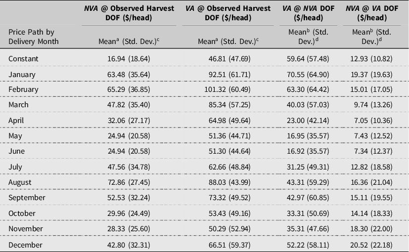
It is not only the opportunity costs of assuming the wrong dynamic profit maximization method that is important but also the assumption of the relevant delivery price path as well. Table 8 reports the opportunity costs of for each profit methodology assuming a constant price path when a seasonal delivery price path is more appropriate. The opportunity costs of assuming constant prices across seasonal delivery price paths for NVA range from $25.14 for December to $33.73/head for June delivery. The opportunity for VA ranges from $15.71 for October and December to $36.17/head for June delivery. Pairwise comparisons across delivery months indicate the influence of a constant price path assumption is typically greater for the NVA than the VA methodology. Overall, the results indicate that the constant price path assumption in Maples resulted in lower opportunity costs of the observed harvest DOF than previously estimated.
Table 8. Opportunity costs of assuming a constant price path † (N = 4,412)
Notes:
† Opportunity costs derived from equation (13). NVA = Non-value Adjusted Method and VA = Value-adjusted Method.
a All paired row means are significantly different at α = .001 based on Wilcoxon Ranked Sum test.
c All paired row variances are significantly different at α = .001.
7. Conclusions
Referred to as a carcass value-adjusted dynamic profit maximization methodology (VA), the study specifically extends Maples et al. (Reference Maples, Coatney, Riley, Karisch, Parish and Vann2015) dynamic profit maximization referred to as a live NVA. By doing so, the study highlights the importance of understanding the influence of the inherent dynamic processes of live weight growth, associated underlying carcass characteristics, and market prices on the optimal market timing of fed cattle. By deriving live cash carcass equivalent prices based on the evolution of the underlying carcass value, the study is more closely aligned to real-world transactions, where both buyers and sellers develop perceived values of the underlying carcass while the cattle are still alive before making buying/selling decisions. Additionally, realistic seasonal price paths contingent on month of delivery are included to better understand the influence of seasonal prices on marketing decisions.
The comparative results between the NVA and VA marketing methods identify the opportunity costs associated with not accounting for the evolution of the carcass and its respective state values. By accounting for the evolution of carcass value, profitability can be improved by mitigating the costs associated with light and heavy weight discounts, as well as under- and over-finished carcasses. The importance of these results to an average producer is that is better to be wrong about the prediction of carcass value than to ignore it all together.
The VA marketing strategy explicitly considers the market signals sent through grid (formula) prices by the packer buyer. Assuming these pricing signals are efficient signals of consumer value, the VA marketing methodology concept may help to improve overall market efficiency, especially given market timing is heavily influenced by evolving prices due to changes in supply and demand throughout the year. The observed gravitation toward peak prices while maintaining carcass output value may in turn contribute to a smoothing and reduction in seasonal price risk.
Feeders are aware that fed cattle carcass characteristics and value evolve over time. The knowledge gap addressed in this research is to identify a more structured approach to account for these aspects. As such, this study is not to be taken as a critique per se of how the TCSCF cattle were marketed. In fact, the VA modeling approach readily acknowledges there is merit to the 0.50-inch backfat rule-of-thumb strategy designed to mitigate carcass discounts and provide the highest quality product. The VA modeling approach is simply a more structured way of thinking about the evolution of the underlying carcass value and profitability. Though the results indicate the cattle in the data would benefit from increased time on feed, it is not conclusive that the cattle would have been able to realize improved profits unless there were/are available alternative production protocols to facilitate longer feeding (e.g., various implant combinations). Also, given cattle can only be slaughtered once, the simulated optimal carcass characteristics could not be verified.
Related to the findings of this research, Maples et al. (Reference Maples, Lusk and Peel2018) note that beef production per animal has been increasing for 40 years and attribute part of that progress to improve feed conversion rates through improvements in genetics, nutrition, and growth promotant technology. Improvements in feed conversion manifest itself through improvements in live weight growth in the NVA and VA models, equations (10) and (11), respectively. By the comparative statics presented in Maples et al. (Reference Maples, Coatney, Riley, Karisch, Parish and Vann2015) that directly apply to this study, increasing marginal physical product via improved growth parameters, ( ${{\bf{g}}_i}$
), necessarily increases optimal DOF, and by extension carcass weight in equation (5). However, Maples et al. (Reference Maples, Lusk and Peel2018) identified an unintended consequence of larger beef carcasses; larger thinner cut steaks that meet a fixed serving size are less preferred by consumers resulting in an estimated $8.6 billion in lost consumer surplus. They acknowledge that consumer surplus losses may be offset to some degree by the increases in beef production efficiency, and in the context of this study the profit incentives of cattle feeders, beef packers notwithstanding.
${{\bf{g}}_i}$
), necessarily increases optimal DOF, and by extension carcass weight in equation (5). However, Maples et al. (Reference Maples, Lusk and Peel2018) identified an unintended consequence of larger beef carcasses; larger thinner cut steaks that meet a fixed serving size are less preferred by consumers resulting in an estimated $8.6 billion in lost consumer surplus. They acknowledge that consumer surplus losses may be offset to some degree by the increases in beef production efficiency, and in the context of this study the profit incentives of cattle feeders, beef packers notwithstanding.
Though as a proof of concept for Angus and Angus cross-bred cattle the VA model shows promise, it has some limitations in specificity. The major limitation is that though the “one size fits all” carcass characteristic prediction equations may be useful for pen average predictions, the accuracy on an individual basis is less than ideal. Improving prediction of individual carcass characteristics based on readily available live weights is warranted. Historically, identification of these relationships has been provided by a sparse collection of serial slaughter studies. The small number of studies is due to the sheer expense of procuring enough cattle conducive for mass analysis of the heterogeneous population of cattle fed in the United States. Alternatively, conducting non-invasive “mock” serial slaughter studies by means of a non-invasive ultrasound technique may prove useful. The goal of such research would be to quantify the relationship between the carcass characteristics to readily observable whole-body weights and other exogenous live cattle characteristics (i.e., breed, sex, origin, and environmental conditions) and carcass characteristics.
Fed cattle producers who are accustomed to sorting market ready cattle are more likely to adopt the VA methodology, such as the smaller Iowa producers in this study. Instead of sorting cattle based on a targeted carcass endpoint, cattle could be grouped by similar marketing dates. However, there exist barriers to widespread adoption of either the NVA or VA methodologies. For example, adoption would require a major paradigm shift for larger feeders who comprise most of the fed cattle sales. It is common practice for large feeders to market fed cattle on a whole pen basis, regardless of whether determined by estimates of carcass value and/or market forces and are less inclined to sort market ready cattle. Additionally, scheduling cattle into slaughter facilities is not a frictionless process and the recent packer shutdowns caused by COVID-19 and the hacking of JBS computers highlights the difficulties of feeders to “optimally” time the market.
Acknowledgements
The authors would like to acknowledge David Trowbridge and Matt Groves for their insightful comments and suggestions.
Financial support
This research received no specific grant from any funding agency, commercial or not-for-profit sectors.
Data Availability Statement
Carcass and feedlot data are propriety and permission must be obtained from Tri County Steer Carcass Futurity Cooperative http://www.tcscf.com/. All other data are public.
Conflict of Interest
None.
Appendix A
A.1 Dress Percentage Conversion Procedure
Bruns et al. (Reference Bruns, Pritchard and Boggs2004) serial slaughter study estimated dressing percent as
 $$DP = .4739 + .0005(HCW)$$
where HCW is in kilograms. Equation (a.1) was estimated by means of a Fisher’s least square ANOVA generated using the GLM procedure in SAS. To express Equation (a.1) in terms of pounds of HCW, a range of HCW (in kilograms) fitting Bruns et al. (Reference Bruns, Pritchard and Boggs2004) was used in Equation (a.1) to estimate DP the respective HCW (in kilograms). The predicted HCW was then multiplied by the conversion factor of 2.20462. Next, the HCW (in pounds) was divided by the corresponding predicted DP from (a.1) to derive an estimated SLW. The estimated SLW was then multiplied by 1.04 to obtain the live weight estimate in pounds. Using the SLW and DP, the following OLS regression was estimated in a pound’s version of (a.1) resulting in the final pounds converted growth equation of
 $$D{P_{it}} = 0.4291 + 0.000185(SL{W_{it}})$$
A.2 Backfat Cover Conversion Procedure
Bruns et al. Reference Bruns, Pritchard and Boggs2004, estimated for backfat cover (FC) (termed “rib fat” in article),
 $$FC = .5442 - .0045(HCW) + .0000202(HCW_{}^2)$$
where HCW is in kilograms and backfat cover is in centimeters. To do the conversion, the same range of HCW (in kilograms) stated above the fat cover in centimeters was calculated using Equation (a.3). Then to convert the backfat from centimeters to inches, backfat was divided by the conversion factor 2.54. The respective HCW (in kilograms) was converted to pounds by multiplying by the conversion factor of 2.20462. Once in pounds (lbs.) the HCW was squared. Finally, an OLS regression was estimated on backfat (in inches) by HCW (in lbs.) and the square of HCW. The resulting equation for backfat cover growth as a function of HCW growth is
 $$F{C_{it}} = 0.{\rm{214252}} - 0.{\rm{000804}}(HC{W_{it}}) + 0.000002(HCW_{it}^2)$$
A.3 Marbling Score Conversion Procedure
Bruns et al. Reference Bruns, Pritchard and Boggs2004 estimated marbling score (MS) is
 $$MS = 60.199 + 1.654(HCW)$$
Equation (a.5) is then converted into pounds as follows. The MS was first predicted from Equation (a.5) by HCW in kilograms. Next, the HCW was converted to pounds by multiplying by the conversion factor 2.20462. Next, an OLS regression was estimated on the originally predicted MS by HCW in pounds. The resulting equation for MS growth as a function of HCW growth is
 $$M{S_{it}} = 60.199 + 0.750243(HC{W_{it}})$$


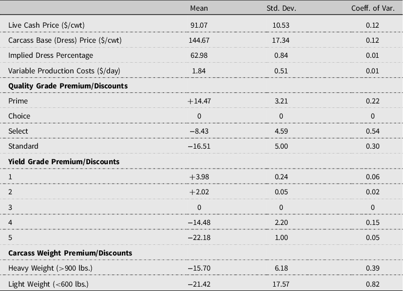


 Open access