


1. Introduction
Transition to turbulence in a boundary layer results in increased wall friction, penalizing aircraft drag. At high speeds, the generated heat is significant and becomes a major concern for the design of supersonic/hypersonic vehicles (Juliano, Borg & Schneider Reference Juliano, Borg and Schneider2015). The transition to turbulence in boundary layers is initiated by amplification of external disturbances of various kinds (roughness, sound waves, free-stream turbulence, etc.), and several paths to transition are possible depending on the nature and intensity of incoming disturbances (Morkovin Reference Morkovin1969). With low levels of disturbances, their growth is described by linear stability theory. The stability of a supersonic boundary layer has been studied widely in the literature (Mack Reference Mack1984; Malik Reference Malik1989; Ma & Zhong Reference Ma and Zhong2003; Bugeat et al. Reference Bugeat, Chassaing, Robinet and Sagaut2019; and many others). For sufficiently high Mach numbers, this configuration is characterized by the presence of two distinct inviscid instability mechanisms: a generalized inflection point for the first Mack mode (Mack Reference Mack1984), and a region where the streamwise base-flow velocity relative to the disturbance phase velocity is supersonic for the second Mack mode, implying that acoustic noise is trapped in this region (Mack Reference Mack1984; Fedorov Reference Fedorov2011). A classical approach for relating instability to transition is based precisely on this linear framework and is called the  $N$-factor method (Smith & Gamberoni Reference Smith and Gamberoni1956), wherein transition is assumed to occur when a perturbation has been amplified by a factor ${\rm e}^{N}$, which defines an energy threshold depending on the disturbance environment.
Numerous studies addressed the problem of transition delay in the supersonic boundary layer flow using active control: Gaponov & Smorodsky (Reference Gaponov and Smorodsky2016) injected heavy gas through porous wall to reduce surface friction and heat transfer, Sharma et al. (Reference Sharma, Shadloo, Hadjadj and Kloker2019) resorted to the generation of streaks to counter transient instabilities, Yao & Hussain (Reference Yao and Hussain2019) investigated the impact of spanwise wall oscillation on the drag of a supersonic turbulent boundary layer, and Jahanbakhshi & Zaki (Reference Jahanbakhshi and Zaki2021) took advantage of the sensitivity of the Mack modes to temperature to delay transition to turbulence. More recently, Celep et al. (Reference Celep, Hadjadj, Shadloo, Sharma, Yildiz and Kloker2022) combined both streak generation and wall heating/cooling effects to control oblique breakdown in a supersonic boundary layer. However, all the aforementioned studies employed predetermined active strategies that do not exploit any real-time measurement and may therefore be less cost-effective and robust to changes in operating conditions than a reactive control strategy (Gad-el Hak Reference Gad-el Hak2000). To the best of our knowledge, reactive control of convective instabilities in a supersonic boundary layer has not yet been considered.
Contrary to oscillator flows (Barbagallo, Sipp & Schmid Reference Barbagallo, Sipp and Schmid2009; Schmid & Sipp Reference Schmid and Sipp2016), which are by definition linearly globally unstable (Huerre & Monkewitz Reference Huerre and Monkewitz1990) and have intrinsic dynamics, noise-amplifier flows like the supersonic boundary layer are extremely sensitive to external disturbances, which are amplified downstream as they are convected by the flow (hence the name convective instabilities). In this context, the purpose of reactive control is to cancel out noise-induced perturbations (Bagheri, Brandt & Henningson Reference Bagheri, Brandt and Henningson2009; Barbagallo et al. Reference Barbagallo, Dergham, Sipp, Schmid and Robinet2012) by producing destructive interferences with an actuator. This task is difficult for mainly two reasons: (a) the detection of the time delay associated with the convection of perturbations that may trigger out-of-phase actions with respect to the incoming perturbations; (b) the wide spatially evolving range of amplified frequencies along the plate, from higher frequencies upstream to lower ones downstream.
1.1. Historical dominance of feedforward/linear–quadratic–Gaussian synthesis for the control of noise-amplifier flows
Controller synthesis is feasible only for models of small dimensions, of the order of  $10^2$ degrees of freedom at most, because of the computational cost and storage requirements of currently available tools (Ramesh, Utku & Garba Reference Ramesh, Utku and Garba1989). Therefore, most fluidic control problems require the identification of reduced-order models (ROMs), using for instance the eigensystem realization algorithm (ERA) on impulse response data. This popular tool, introduced by Juang & Pappa (Reference Juang and Pappa1985), has already been used in many control studies for noise-amplifier flows (Belson et al. Reference Belson, Semeraro, Rowley and Henningson2013; Dadfar et al. Reference Dadfar, Semeraro, Hanifi and Henningson2013; Sasaki et al. Reference Sasaki, Morra, Cavalieri, Hanifi and Henningson2020; and many others). Once ROMs are obtained, the control law is built with classical tools of control theory that are mathematically well-established in a linear framework and thus perfectly suited for controlling the linear growth of small perturbations.
In noise-amplifier flows, there is no synchronization of the dynamics at a global scale, and perturbations from an actuator  $u$ are rapidly damped in the upstream direction, hence the control set-up changes fundamentally depending on the position of the estimation sensor $y$ relative to $u$. When $y$ is placed upstream, actuator-induced perturbations are not observable, and the configuration is termed ‘feedforward’ (Bagheri et al. Reference Bagheri, Brandt and Henningson2009; Semeraro et al. Reference Semeraro, Bagheri, Brandt and Henningson2011; Hervé et al. Reference Hervé, Sipp, Schmid and Samuelides2012; Juillet, Schmid & Huerre Reference Juillet, Schmid and Huerre2013; Morra et al. Reference Morra, Sasaki, Hanifi, Cavalieri and Henningson2020). On the other hand, when $y$ is placed downstream, the sensor measures the superposition of noise-induced and actuator-induced perturbations, hence the term ‘feedback’ (Barbagallo et al. Reference Barbagallo, Dergham, Sipp, Schmid and Robinet2012; Belson et al. Reference Belson, Semeraro, Rowley and Henningson2013; Semeraro et al. Reference Semeraro, Pralits, Rowley and Henningson2013b; Vemuri et al. Reference Vemuri, Bosworth, Morrison and Kerrigan2018; Tol, Kotsonis & de Visser Reference Tol, Kotsonis and de Visser2019). In this case, though, there may be a significant time delay before the effect of actuation may be seen by the sensor, because perturbations are convected at a finite rate by the underlying base flow: the farther downstream $y$ is, the longer the delay.
The literature on noise-amplifier control is dominated by the linear–quadratic–Gaussian (LQG) synthesis (Semeraro et al. Reference Semeraro, Bagheri, Brandt and Henningson2011; Barbagallo et al. Reference Barbagallo, Dergham, Sipp, Schmid and Robinet2012; Juillet et al. Reference Juillet, Schmid and Huerre2013; Sasaki et al. Reference Sasaki, Morra, Fabbiane, Cavalieri, Hanifi and Henningson2018a; Tol et al. Reference Tol, Kotsonis and de Visser2019; and many others), a synthesis method dating back to the 1960s (Kalman Reference Kalman1964). Despite being theoretically optimal with respect to a performance criterion, this method comes with no guarantees on stability margins (Doyle Reference Doyle1978). In other words, tiny errors in the model may end up with an unstable feedback loop when  $y$ is placed downstream of $u$ (feedback set-up), which represents a major drawback for practical applications. Using the loop-transfer-recovery method, it is in some cases possible to overcome this lack of stability robustness by overwhelming the control signal entering the estimator (Kwakernaak Reference Kwakernaak1969; Doyle & Stein Reference Doyle and Stein1981). This procedure has, for example, been used successfully by Sipp & Schmid (Reference Sipp and Schmid2016) to improve the stability robustness of their controller in the case of a flow over an open square cavity (oscillator flow). The recovery procedure works by inverting the plant dynamics in order to obtain ultra-fast estimators. This procedure leads to an unstable closed loop in the case of systems with time delays, because they possess right-half-plane zeros that are converted into right-half-plane poles (Zhang & Freudenberg Reference Zhang and Freudenberg1987; Skogestad & Postlethwaite Reference Skogestad and Postlethwaite2005; Sipp & Schmid Reference Sipp and Schmid2016). As a result, this method is not suitable for noise-amplifier flows in general, and in particular, the supersonic boundary layer flow. Contrary to the feedback structure, the feedforward design is unconditionally stable, and its implementation via LQG synthesis is not a problem. Therefore, feedforward configurations combined with LQG syntheses dominate the noise-amplifier flow control literature, particularly in the incompressible boundary layer control studies (Bagheri et al. Reference Bagheri, Brandt and Henningson2009; Semeraro et al. Reference Semeraro, Bagheri, Brandt and Henningson2011, Reference Semeraro, Bagheri, Brandt and Henningson2013a,Reference Semeraro, Pralits, Rowley and Henningsonb; Dadfar et al. Reference Dadfar, Semeraro, Hanifi and Henningson2013, Reference Dadfar, Fabbiane, Bagheri and Henningson2014; Sasaki et al. Reference Sasaki, Morra, Fabbiane, Cavalieri, Hanifi and Henningson2018a, Reference Sasaki, Morra, Cavalieri, Hanifi and Henningson2020; Freire et al. Reference Freire, Cavalieri, Silvestre, Hanifi and Henningson2020; Morra et al. Reference Morra, Sasaki, Hanifi, Cavalieri and Henningson2020).
1.2. Feedforward ‘Achilles heel’: performance robustness
However, the use of a feedforward set-up raises the problem of robustness to performance, which can be defined as the control law's ability to remain efficient in terms of perturbation amplitude reduction despite modelling errors or free-stream condition variations around the reference case. This problem has been little addressed in the boundary layer control literature, despite the advent of robust synthesis, introduced by Doyle et al. (Reference Doyle, Glover, Khargonekar and Francis1989). So far, these modern methods have been used mainly in the case of oscillator flows (Flinois & Morgans Reference Flinois and Morgans2016; Leclercq et al. Reference Leclercq, Demourant, Poussot-Vassal and Sipp2019; Shaqarin et al. Reference Shaqarin, Oswald, Noack and Semaan2021) to have some stability guarantees, because using a feedback set-up is mandatory to stabilize a globally unstable flow.
To improve performance robustness compared to a simple fixed-structure LQG feedforward controller, Erdmann et al. (Reference Erdmann, Pätzold, Engert, Peltzer and Nitsche2011) and Fabbiane et al. (Reference Fabbiane, Semeraro, Bagheri and Henningson2014, Reference Fabbiane, Simon, Fischer, Grundmann, Bagheri and Henningson2015) used an adaptive feedforward method for boundary layer control, based on the filtered-X least-mean-squares (FXLMS) algorithm, where the controller structure is adjusted according to the variations of the flow conditions through real-time measurements. However, this method is not robust to abrupt changes in inflow conditions because the controller coefficients are adjusted in a quasi-static fashion. Due to its natural ability to be robust to unknown disturbances or uncertainties on the model (Skogestad & Postlethwaite Reference Skogestad and Postlethwaite2005), feedback design appears to be a promising alternative for performance robustness on short time scales. Barbagallo et al. (Reference Barbagallo, Dergham, Sipp, Schmid and Robinet2012) employed a feedback structure combined with an LQG synthesis to control instabilities over a backward-facing step, and emphasized the importance of placing the estimation sensor close to the actuator to obtain a reasonable performance. Doing so increases the controllable bandwidth indeed, as it is limited in feedback set-up by the convection delay of the disturbances from the actuator to the estimation sensor. However, some of their feedback controllers turned out to be unstable on the real plant (the full linearized Navier–Stokes equations), because of the poor stability robustness of LQG synthesis to tiny errors in the ROM. Tol et al. (Reference Tol, Kotsonis and de Visser2019) also obtained some unstable controllers when trying to control Tollmien–Schlichting (TS) waves in an incompressible two-dimensional (2-D) boundary layer using LQG synthesis on a feedback set-up. Belson et al. (Reference Belson, Semeraro, Rowley and Henningson2013) are among the first to demonstrate the feasibility of a feedback set-up with stability and performance robustness for the same flow, using a simple proportional integral (PI) controller that was tuned by hand. However, the simple structure of the PI controller did not allow them to obtain a satisfactory performance for the chosen actuator/sensor pair, forcing the authors to change it, despite the good performance obtained with LQG synthesis on the ROMs with the same actuator/sensor pair. A similar approach was used by Vemuri et al. (Reference Vemuri, Bosworth, Morrison and Kerrigan2018) in order to cancel out TS waves in an experimental set-up. The authors tuned a proportional controller by hand to optimize the controller gain in a closed loop while ensuring robust stability of their feedback configuration. Such loop-shaping approaches provide guarantees on stability robustness but are far from optimal from a performance viewpoint. And perhaps more importantly, they are very limited in the sense that they cannot be applied to more complex controller structures in a systematic way.
1.3. Designing robust controllers: structured mixed  $H_{2}$/$H_{\infty }$ synthesis techniques


In contrast, modern tools for robust multi-criteria synthesis, such as the structured mixed  $H_{2}$/ $H_{\infty }$ synthesis (Apkarian, Gahinet & Buhr Reference Apkarian, Gahinet and Buhr2014), allow us to optimize complex control laws. The structured mixed $H_{2}$/ $H_{\infty }$ synthesis is able to treat different kinds of mathematical criteria simultaneously, contrary to the LQG method, which minimizes a single quadratic criterion based on performance and cost. Furthermore, structured synthesis (Apkarian & Noll Reference Apkarian and Noll2006) has the advantage of limiting the controller order and imposing its structure beforehand (e.g. state-space model of order 10, proportional integral derivative controller, etc.), unlike methods that solve Riccati equations, such as LQG (Freire et al. Reference Freire, Cavalieri, Silvestre, Hanifi and Henningson2020), $H_{\infty }$ (Flinois & Morgans Reference Flinois and Morgans2016) or $H_{2}$ (Tol et al. Reference Tol, Kotsonis, De Visser and Bamieh2017) optimal controls, which lead to high-order controllers (of the same order as the plant augmented by weighting functions). These are often too expensive to use in real-time applications, and require reducing the controller order in a post-processing step. Performing this reduction optimally while maintaining stability and performance guarantees on the closed loop remains an open problem (Chen, Zhou & Chang Reference Chen, Zhou and Chang1994; Goddard & Glover Reference Goddard and Glover1995). The possibility of working with both $H_{2}$ (an integrated gain over all frequencies) and $H_\infty$ (the maximum gain over all frequencies) criteria ensures performance, robustness to stability and robustness to performance (Apkarian, Noll & Rondepierre Reference Apkarian, Noll and Rondepierre2010). Indeed, the use of $H_{\infty }$ criteria on some transfer functions allows us to respect stability margins on the feedback design (what was missing within the LQG synthesis) despite modelling errors, and to desensitize the controller on certain frequency ranges, allowing optimal performance to be maintained despite the presence of, for example, noise on the estimation sensor. The use of $H_{2}$ criteria makes it possible to have a performance objective of disturbance rejection during the synthesis (which was sometimes lacking in previous feedback studies).
1.4. Objective and outline of the paper
In the present paper, we will consider a supersonic boundary layer at  $M=4.5$ and focus on 2-D (i.e. spanwise-invariant) and linear perturbations. We will not be dealing with oblique modes or finite-amplitude perturbations, even if they often do play a significant role in transition in practice. Hence the present work is only a first step in learning how to design robust control laws for the problem of transition in the supersonic boundary layer. One key question that we wish to address before introducing more physical complexity is how do the feedforward and feedback set-ups compare on this noise-amplifier flow, using modern robust synthesis tools? With the help of multi-criteria structured $H_{2}$/ $H_{\infty }$ controller synthesis, can we design a feedback set-up that outperforms the often-used feedforward/LQG synthesis with regards to performance robustness to realistic changes in operating conditions, i.e. velocity and density variations?
The paper is organized as follows. Sections 2 and 3 provide a description of the flow configuration and numerical methods. In § 4, local and global linear stability tools are used to define appropriate closed-loop specifications, i.e. determining the actuators, sensors and performance criterion to be optimized. Section 5 is devoted to ROM identification from impulse responses using the ERA, with special emphasis on the problem of time delays in such noise-amplifier flows. Next, we formally introduce the multi-criteria structured mixed  $H_{2}$/ $H_{\infty }$ synthesis and the associated constraint minimization problem that we wish to solve. In § 6, we compare the results obtained on and off design (noisy sensors, density and velocity variations) for the feedforward and feedback set-ups. Conclusions are drawn in § 7.
2. Flow configuration
A 2-D compressible ideal gas flowing over a flat plate is considered. The flow is governed by the Navier–Stokes equations:
 $$\begin{gather} \frac{\partial \rho }{\partial t}+\boldsymbol{\nabla}\boldsymbol{\cdot}(\rho\boldsymbol{u})=0, \end{gather}$$
 $$\begin{gather}\frac{\partial \rho\boldsymbol{u} }{\partial t}+\boldsymbol{\nabla}\boldsymbol{\cdot}(\rho\boldsymbol{u}\otimes\boldsymbol{u})={-}\boldsymbol{\nabla} p +\boldsymbol{\nabla}\boldsymbol{\cdot}\boldsymbol{\tau}, \end{gather}$$
 $$\begin{gather}\frac{\partial \rho E}{\partial t}+\boldsymbol{\nabla}\boldsymbol{\cdot}(\rho E\boldsymbol{u})=\boldsymbol{\nabla}\boldsymbol{\cdot}(- p\boldsymbol{u}+\boldsymbol{\tau }\boldsymbol{\cdot}\boldsymbol{u}-\boldsymbol{\theta}), \end{gather}$$
where  $\rho$ is the fluid density, $\boldsymbol {u}$ is the velocity vector, $p$ is the static pressure, $E={p}/{\rho (\gamma -1)}+{(\boldsymbol {u}\boldsymbol {\cdot }\boldsymbol {u})}/{2}$ is the total energy, $\boldsymbol {\tau }$ is the viscous stress tensor, and $\boldsymbol {\theta }$ is the heat flux vector. The viscous stress tensor and the heat flux vector are given by
 $$\begin{gather} \boldsymbol{\tau}=\mu\left(\boldsymbol{\nabla} \otimes \boldsymbol{u} +(\boldsymbol{\nabla} \otimes \boldsymbol{u})^{\rm T} -\tfrac{2}{3}(\boldsymbol{\nabla} \boldsymbol{\cdot}\boldsymbol{\boldsymbol{u}})\boldsymbol{\mathsf{I}}\right), \end{gather}$$
 $$\begin{gather}\boldsymbol{\theta}={-}k\,\boldsymbol{\nabla}T, \end{gather}$$
with  $\boldsymbol{\mathsf{I}}$ the identity tensor, $k$ the thermal conductivity, and $\mu$ the dynamic viscosity, which is deduced from the local temperature $T$ via Sutherland's law,
 \begin{equation} \mu=\mu_{ref}\left(\frac{T}{T_{ref}}\right)^{{3}/{2}}\frac{T_{ref}+S}{T+S}. \end{equation}
The parameters of Sutherland's law are taken as  $\mu _{ref}=1.716 \times 10^{-5}\ \mathrm {Pa\ s}$, $T_{ref}=273.15\ \mathrm {K}$ and $S=110.4\ \mathrm {K}$. The gas considered being air, we have $\gamma =1.4$, $r=287\ \mathrm {J\ K^{-1}\ kg^{-1}}$ and $Pr={\mu \gamma r}/{k(\gamma -1)}=0.725$. The free-stream flow conditions are very close to those used experimentally by Kendall (Reference Kendall1975) and in the simulations of Ma & Zhong (Reference Ma and Zhong2003), i.e. $T_{\infty }=65.149 \ \mathrm {K}$, $U_{\infty }=728.191\ \mathrm {m\ s^{-1}}$ and $p_{\infty }=728.312\ \mathrm {Pa}$. Thus the free-stream Mach number of the simulation is $M_{\infty }={U_{\infty }}/{\sqrt {\gamma rT_{\infty }}}=4.5$.
The computational domain is represented in figure 1(a). It consists of a rectangular domain where the lower boundary is an adiabatic flat plate of length  $L_{x}=2002.1\delta _{0}^{*}$, with $\delta _{0}^{*}=3.2656 \times 10^{-4}\ \mathrm {m}$ the compressible displacement thickness at the inlet of the domain (defined as $\delta _{0}^{*}=\int ^{\infty }_{0} (1-{\rho u}/{\rho _{\infty }u_{\infty }})\,{\rm d} y$), which results in $Re_{\delta _0^*}={\rho _{\infty }U_{\infty }\delta _0^*}/{\mu _{\infty }}\approx 2121$.

Figure 1. (a) Diagram of the computational domain. Inputs and outputs of the control problem are in red and blue, respectively. (b) Boundary layer profile used for the inlet condition.
Far-field and supersonic exit conditions are respectively applied at the top ( $y=275\delta _{0}^{*}$) and at the outlet of the computational domain. Furthermore, a sponge area is used downstream and in the upper part of the domain to minimize reflections. This sponge area has length $L_{sponge}=91.9\delta _{0}^{*}$ in both streamwise and wall-normal directions; it consists in adding a source term in (2.1) on the last 10 cells closest to the boundaries to bring the flow back to its equilibrium point. In addition, the mesh is stretched in the longitudinal direction for the downstream boundary (30 cells in the streamwise direction). A supersonic inlet condition is imposed at the upstream boundary where the complete state is prescribed and matches a zero-pressure gradient laminar boundary layer profile (see figure 1b) computed with the ONERA boundary layer code CLICET (see, for instance, Olazabal-Loume et al. Reference Olazabal-Loume, Danvin, Mathiaud and Aupoix2017). It corresponds to a profile taken at distance $19\delta _{0}^{*}$ from the leading edge. The beginning of the numerical domain has been chosen to be in a stable area for all frequencies according to local linear stability theory (see § 4.1). The boundary layer thickness (denoted $\delta$) at the end of the domain of interest leads to $Re_{\delta }\approx 35\,081$. Overall, the useful numerical domain (i.e. not counting the length of the sponge area) extends over $4\times 10^{4}< Re_{x}={\rho _{\infty }U_{\infty }x}/{\mu _{\infty }}<4.1\times 10^{6}$.
3. Base-flow and spatial stability analyses
3.1. Base flow and linearized DNS
Direct numerical simulations (DNS) are performed using the finite volume code elsA (Cambier, Heib & Plot Reference Cambier, Heib and Plot2013). An upwind AUSM + up scheme (Liou Reference Liou2006) associated with a third-order MUSCL extrapolation method (van Leer Reference van Leer1979) is used for the spatial discretization of the convective fluxes. The viscous fluxes are obtained by a second-order centred scheme. The semi-discretized Navier–Stokes equations then read
 \begin{equation} \frac{{\rm d} \boldsymbol{q}}{{\rm d} t}=\boldsymbol{\mathsf{N}}(\boldsymbol{q})+\boldsymbol{\mathsf{P}}\boldsymbol{f}, \end{equation}
where  $\boldsymbol {q}=[\rho, \rho \boldsymbol {u}, \rho E]^{\rm T}$, and $\boldsymbol{\mathsf{N}}(\boldsymbol {q})$ is the discretized compressible Navier–Stokes equations (including the boundary conditions). The momentum forcing $\boldsymbol {f}$ may represent either a noise source or the effect of an actuator. The matrix $\boldsymbol{\mathsf{P}}$ represents the prolongation operator that transforms the momentum forcing into a full state-vector forcing by adding zero components. The laminar base flow $\bar {\boldsymbol {q}}$, defined as
 \begin{equation} \boldsymbol{\mathsf{N}}(\bar{\boldsymbol{q}})=0, \end{equation}
is obtained by time stepping the unforced unsteady (3.1) with an implicit time-stepping method based on a local time step, up to convergence of the residuals. The unsteady simulations for the development of instabilities are performed with an implicit second-order Gear scheme (Gear Reference Gear1971) with four sub-iterations and a time step  ${\rm d}t$ ensuring a Courant–Friedrichs–Lewy number lower than $1.4$ in the whole domain. For these unsteady simulations, the amplitude of the forcing $\boldsymbol {{f}}$ is chosen sufficiently small to ensure that the induced perturbation $\boldsymbol {q}'=\boldsymbol {{q}}-\bar {\boldsymbol {q}}$ remains in the linear regime until the end of the computational domain. The time step and the number of sub-iterations of the temporal method have been validated by comparing transfer functions from the linearized DNS and those determined from the frequency-domain resolvent approach (defined in § 3.2).
A resolution of  $3200\times 220$ cells for the useful domain is chosen. The mesh is uniform in the $x$ direction, while a geometric law is used in the $y$ direction to resolve strong gradients near the wall. The base-flow and linear growth rates have been verified against the linearized DNS results of Ma & Zhong (Reference Ma and Zhong2003), allowing us to validate the resolution and the numerical schemes (see Appendix A).
3.2. Global resolvent analysis
For purposes of controlling instabilities, the choice of the type and position of the actuator/sensors will play an essential role. This choice is guided by resolvent analysis, which characterizes the noise-amplifier behaviour from an input–output viewpoint. The method is detailed briefly in this subsection.
The purpose of control is to reduce the amplitude of disturbances that develop naturally in the boundary layer, and thus to maintain the flow as close as possible to its equilibrium  $\bar {\boldsymbol {q}}$. By injecting the ansatz $\boldsymbol {{q}}=\bar {\boldsymbol {q}}+\boldsymbol {q}'$ into (3.1) and considering only small-amplitude forcing $\boldsymbol {f}$, we obtain after linearization that
 \begin{equation} \frac{{\rm d} \boldsymbol{q}'}{{\rm d} t}=\boldsymbol{\mathsf{A}}\boldsymbol{q}'+\boldsymbol{\mathsf{P}}\boldsymbol{f}, \end{equation}
where  $\boldsymbol{\mathsf{A}}$ is the Jacobian matrix defined as $\boldsymbol{\mathsf{A}}={{\rm d} \boldsymbol{\mathsf{N}}}/{{\rm d} \boldsymbol {q}}|_{\bar {\boldsymbol {q}}}$. In our configuration, all the eigenvalues of $\boldsymbol{\mathsf{A}}$ have a negative real part, and the flow is therefore globally stable. Switching to the frequency domain, a direct relation between the spatial structure of a harmonic forcing $\boldsymbol {f}(x,y,t)=\tilde {\boldsymbol {f}}(x,y)\,{\rm e}^{{\rm i}\omega t}$ and its flow response $\boldsymbol {q}'(x,y,t)=\tilde {\boldsymbol {q}}(x,y)\,{\rm e}^{{\rm i}\omega t}$ is established:
 \begin{equation} \tilde{\boldsymbol{q}}=\boldsymbol{\mathsf{R}}\tilde{\boldsymbol{f}}, \end{equation}
where  $\boldsymbol{\mathsf{R}}=({\rm i}\omega \boldsymbol{\mathsf{I}} -\boldsymbol{\mathsf{A}})^{-1}\boldsymbol{\mathsf{P}}$ is the resolvent operator, and $\omega =2{\rm \pi} f \in \mathbb {R}$ is the angular frequency. For a given frequency and among all the possible forcings, we examine the one that maximizes the gain:
 \begin{equation} \tilde{g}^{2}(\omega)=\sup_{\tilde{\boldsymbol{f}} \neq 0}\frac{\|\tilde{\boldsymbol{q}}\|^{2}_{E}}{\|\tilde{\boldsymbol{f}}\|^{2}_{F}}, \end{equation}
where  $\|\cdot \|^{2}_{E}$ and $\|\cdot \|^{2}_{F}$ respectively denote the Chu energy norm and the energy of the momentum forcing (Bugeat et al. Reference Bugeat, Chassaing, Robinet and Sagaut2019). The Chu energy is defined as
 \begin{equation} E_{Chu}=\frac{1}{2}\int_{\mathcal{V}} \left(\overbrace{\underbrace{\bar{\rho}(|{u'}|^{2}+|{v'}|^{2}}_{e_{u'}}) +\underbrace{r\,\frac{\bar{T}}{\bar{\rho}}\,|\rho'|^{2}}_{e_{\rho'}} +\underbrace{\frac{r}{\gamma-1}\,\frac{\bar{\rho}}{\bar{T}}\,|T'|^{2}}_{e_{T'}}}^{e_{Chu}}\right){\rm d}V; \end{equation}
it contains terms relative to thermodynamic perturbations in addition to the kinetic one, and is therefore commonly used to study the global behaviour of compressible flows (Hanifi, Schmid & Henningson Reference Hanifi, Schmid and Henningson1996; Bugeat et al. Reference Bugeat, Chassaing, Robinet and Sagaut2019). For a given frequency, the fields  $\tilde {\boldsymbol {f}}$ and $\tilde {\boldsymbol {q}}$ corresponding to the optimal gain $\tilde {g}$ are respectively called optimal forcing and response modes. Determining the optimal gain amounts to computing the largest eigenvalue of a positive generalized eigenvalue problem with the Arnoldi algorithm (ARPACK library, Lehoucq, Sorensen & Yang Reference Lehoucq, Sorensen and Yang1998) using a sparse LU solver (MUMPS library, Amestoy et al. Reference Amestoy, Duff, L'Excellent and Koster2001) for linear system solution. The Jacobian matrix $\boldsymbol{\mathsf{A}}={{\rm d} \boldsymbol{\mathsf{N}}}/{{\rm d} \boldsymbol {q}}|_{\bar {\boldsymbol {q}}}$ is extracted explicitly using a second-order finite-difference method (Beneddine Reference Beneddine2017). This global analysis tool developed in previous work (Beneddine, Mettot & Sipp Reference Beneddine, Mettot and Sipp2015) was validated on the supersonic boundary layer results of Bugeat et al. (Reference Bugeat, Chassaing, Robinet and Sagaut2019). In our study, the domains involved in the definition of $\|\cdot \|^{2}_{E}$ and $\|\cdot \|^{2}_{F}$ correspond to both $x\in [0;1910.2\delta _{0}^{*}]$ and $y\in [0;92\delta _{0}^{*}]$.
3.3. Local stability analysis
The primary aim of the local linear stability theory (LLST) for the present study is to classify the mechanisms involved in our DNS and resolvent analysis by associating local modal mechanisms from the LLST with those observed in our purely non-modal DNS and global resolvent study. Indeed, the flow being globally stable, the growth of disturbances is due only to non-modal phenomena. These non-modal effects are a consequence of the non-normality of  $\boldsymbol{\mathsf{A}}$ (Schmid Reference Schmid2007). The non-normal effects can be cast in two categories for open-flows: the component-type non-normality, and the convective-type non-normality (Sipp et al. Reference Sipp, Marquet, Meliga and Barbagallo2010). Component-type non-normality is characterized by a componentwise transfer of energy between the forcing and response fields, like in the Orr or lift-up mechanisms (Bugeat et al. Reference Bugeat, Chassaing, Robinet and Sagaut2019) – but note that the latter is absent here since lift-up is three-dimensional (3-D). Convective-type non-normality is caused by modal amplification on the local scale and is characterized by a separation of the spatial supports of the forcing and response fields.
In LLST, we consider perturbations that are evolving very rapidly in the  $x$ direction compared to the base flow. At each streamwise position, the base flow is considered frozen with respect to the perturbations $\phi '=[\rho ',u',v',T']$, therefore the latter can be sought in the form
 \begin{equation} \phi'=\tilde{\phi}(y)\,{\rm e}^{{\rm i}(\alpha x-\omega t)},\end{equation}
where in general the wavenumber  $\alpha$ and the frequency $\omega$ are complex numbers. Plugging this ansatz into the linearized Navier–Stokes equations with frozen base-flow profile leads to a different dispersion relation $D(\alpha,\omega ;x)=0$ for each value of $x$. In the spatial stability framework, we consider real angular frequencies $\omega$ and solve for the complex wavenumber $\alpha =\alpha _r+{\rm i}\alpha _i$, where $\alpha _r$ is the wavenumber, and $-\alpha _i$ is the spatial growth rate along $x$. All perturbations are assumed to vanish at the free-stream boundary $y\to \infty$, while on the flat plate, $y=0$, $\tilde {u}=\tilde {v}=0$ and $\mathrm {d}\tilde {\rho }/\mathrm {d} y=\mathrm {d}\tilde {T}/\mathrm {d} y=0$ (adiabatic plate). Equations are discretized along the wall-normal direction $y$ using a Chebyshev collocation method. For all values of $x$ and $\omega$, an eigenvalue problem is solved, using the LAPACK library, in order to determine the complex eigenvalue $\alpha$ and corresponding eigenvector $\tilde {\phi }=[\tilde {\rho },\tilde {u},\tilde {v},\tilde {T}]$. The analysis is performed using an in-house code detailed fully in Saint-James (Reference Saint-James2020) and validated here by comparing with the linear local growth rates of the supersonic boundary layer from Ma & Zhong (Reference Ma and Zhong2003).
4. Noise-amplifier behaviour and control set-up
4.1. Characterization of instabilities
The local spatial stability diagram of spanwise-invariant perturbations is displayed in figure 2(a), with  $F=2{\rm \pi} f\delta _{0}^{*}/U_{\infty }$ the dimensionless frequency. It is characterized by two distinct instability regions (i.e. where the spatial growth rate is positive, $-\alpha _i>0$): one for the first Mack mode, and one for the second Mack mode. For each mode, the instability domain (depicted by the red solid line) for a given frequency is located between branch I (convectively stable/unstable boundary) and branch II (convectively unstable/stable boundary). Each frequency is therefore amplified only on a certain portion of the domain: high frequencies are amplified upstream, while low frequencies are found further downstream. Compared to the first mode, the unstable frequencies of the second mode are higher and are associated with higher growth rates. Transition to turbulence is often predicted from LLST using the $N$-factor (Smith & Gamberoni Reference Smith and Gamberoni1956)
 \begin{equation} N(\omega,x)=\int_{x_{c}}^{x}-\alpha_{i}(\omega)\,{\rm d} x=\ln\left(\frac{|\phi'|}{|\phi'|_{c}}\right), \end{equation}
with  $x_{c}$ the location of branch I for the considered frequency, and $|\phi '|_{c}$ the amplitude of the mode at this location. The
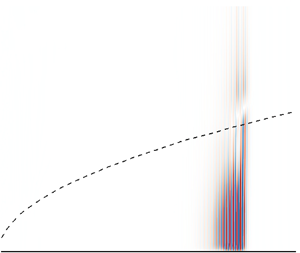
  $N$-factors for different frequencies are represented in figure 2(b). Although the instability range of the first Mack mode is larger, the $N$-factors of the second mode are greater all along the domain due to their higher growth rates. Transition is often assumed to occur when the quantity $\tilde {N}(x)=\max _{\omega } N(\omega,x)$ (red solid lines in figures 2b,c) at the position $x_t$ reaches a threshold value $N_{t}$ (dashed lines in figures 2b,c, placed arbitrarily for the explanation). This criterion means that the transition process begins when a perturbation has been amplified by a factor ${\rm e}^{N_{t}}$. Thus in order to delay transition to turbulence, when $x>x_t$, a control action should transform the quantity $\tilde {N}$ obtained without control into the quantity $\tilde {N}^{c}$ (blue line in figure 2d) with control, such that $\tilde {N}^{c}< N_{t}$ for as long as possible (see figure 2d). The dominant frequency being different at each streamwise location of the domain, a large frequency range needs to be controlled, which complicates the design of the control law. The $\tilde {N}^{c}< N_{t}$ criterion could be translated directly into an $H_{\infty }$ criterion, because this would mean that the maximum amplification over the entire frequency spectrum must not exceed a threshold over the entire domain, exactly as in the $N$-factor method. However, this method may be considered conservative as it is based on the worst perturbation, which is purely harmonic and therefore not quite realistic (Mack Reference Mack1977). Fedorov & Tumin (Reference Fedorov and Tumin2022) recommended instead the use of a criterion based on both the $N$-factors and the entire frequency spectrum of the incoming disturbance $|\phi '|_{c}$, which amounts to considering an $H_{2}$ norm rather than an $H_{\infty }$ norm. We follow this recommendation and choose a performance objective based on an $H_{2}$ norm. More precisely, our objective will be to maintain the spatially integrated amplification below a given threshold along the plate, and this integrated amplification will be quantified using an $H_{2}$ norm (see figure 2d).

Figure 2. (a) Stability diagram; red solid lines represent isolines  $\alpha _{i}=0$. (b) Calculation of the $N$-factors (black solid lines) for transition prediction based on LLST: transition occurs at $x_t$ when $\tilde {N}>N_{t}$ (notional diagram).(c) Performance objective for closed-loop control based on the $N$-factor criterion. (d) Modification of the $N$-factor criterion using the $H_{2}$ norm, in order to reduce conservatism. The quantity $F=2{\rm \pi} f\delta _{0}^{*}/U_{\infty }$ represents the dimensionless frequency.
The global stability results based on resolvent analysis complement those obtained previously from LLST. The optimal energy gain  $\tilde {g}$ as a function of the forcing frequency $F$ is represented in figure 3(a). This curve displays two peaks at $F\approx 0.118$ and $F\approx 0.237$, which correspond respectively to the first and second Mack modes identified in LLST. Global resolvent analyses are consistent with those of the local approach, since the optimal energy gain is closely related to $N$-factors (Sipp et al. Reference Sipp, Marquet, Meliga and Barbagallo2010; Beneddine et al. Reference Beneddine, Mettot and Sipp2015).

Figure 3. (a) Optimal resolvent gain as a function of the dimensionless frequency  $F$. According to LLST, red and green dashed areas represent the unstable frequency range of first and second Mack modes, respectively. The region where both modes are unstable corresponds to an area where the first mode is unstable over a tiny distance. (b) Real part of the streamwise component of the optimal forcing and (c) its associated streamwise velocity response, at $F=0.237$. (d) Evolution at $F=0.237$ of the forcing density and the different contributions to the Chu energy density normalized by their maximum values. The positions of branches I and II from LLST are symbolized by vertical dashed lines. (e) Comparison of $-\alpha _{i}$ and $-\tilde {\alpha }_{i}$ at $F=0.237$.( f) Profiles of the optimal forcing components at $x=867.2\delta _{0}^{*}$, and (g) response at $x=1766.7\delta _{0}^{*}$, at $F=0.237$. The black dashed and dashed-dotted lines in (b), (c), ( f) and (g) represent respectively the generalized inflection point position and the limit of the region of supersonic instabilities ( $\hat {M}>1$ below this line).
For the frequency  $F=0.237$ leading to the highest gain, the real parts of the streamwise optimal forcing and velocity response are shown in figures 3(b,c). The spatial structure of the forcing is located upstream of the domain, while that of the response is located further downstream. This separation of the spatial supports, related to the convective-type non-normality of the Jacobian operator, implies a time delay between actuation upstream and sensing downstream, making the design of a robust control law even more complex. Figure 3(d) shows that the peak of the forcing density $d_{e_{f}}(x)=\int _{0}^{y=92\delta _{0}^{*}} \|\tilde {\boldsymbol {f}}\|^{2}\,{\rm d} y$ (resp. Chu energy density $d_{e_{Chu}}(x)=\int _{0}^{y=92\delta _{0}^{*}} e_{Chu}\,\mathrm {d} y$) is not very far from the position of branch I (resp. II) from LLST (Sipp et al. Reference Sipp, Marquet, Meliga and Barbagallo2010). The energy of the response is dominated at each abscissa by the thermodynamic quantities $e_{T'}$ and $e_{\rho '}$, while quantity $e_{u'}$ has a smaller contribution. Note that the most amplified frequencies depend on the extent of the domain used in the optimization problem (not shown here): the longer the domain, the lower the dominant frequency. The gain of the frequencies that already reach their peak of forcing density and Chu energy density (linked to the positions of branches I and II, respectively) does not vary with an increase of the domain size in the streamwise direction as these frequencies can no longer be amplified. For all the other frequencies (which are lower), the phenomenon of amplification continues, leading to higher gains for a wider area.
A comparison between the spatial amplification rates  $-\alpha _{i}$ from LLST (red dashed line) and $-\tilde {\alpha }_{i}=({1}/{|\tilde {u}(x,y=1.7\delta _{0}^{*})|})\partial _x |\tilde {u}(x,y=1.7\delta _{0}^{*})|$ from resolvent analysis (black dashed line) is depicted in figure 3(e). The quantity $-\tilde {\alpha }_{i}$ represents the slope of $\ln {|\tilde {u}|}$ with respect to $x$ (black solid line) and can therefore be compared to a growth rate; when the convective-type non-normality effects dominate, this growth rate is independent of the choice of $y$ and the primitive variable. The growth of the resolvent mode within $x\in [0;1078\delta _{0}^{*}]$ is due to the optimal forcing that is non-zero in this region (see figure 3d) and that induces the response. The inclined pattern in the forcing field (see figure 2b) indicates that the response also takes advantage of the Orr mechanism (Orr Reference Orr1907) and more generally of non-modal local interactions. After this initial growth region induced by the forcing, both $-\alpha _{i}$ and $-\tilde {\alpha }_{i}$ exhibit similar values in the region in $x\in [1200\delta _{0}^{*};1730\delta _{0}^{*}]$, which indicates that transient growth is then dominated by the convective instability associated with the second Mack mode.
To maximize the amplification of the second Mack mode, the forcing field (see figures 3b, f) must be localized near the generalized inflection point  $y_{g}$ (denoted in figures 3b,c, f,g with a dashed line), defined as $\partial _y (\bar {\rho }\,\partial _y \bar {u})|_{y_{g}}=0$. A region of supersonic instabilities (below the dashed-dotted line in figures 3b,c, f,g) – defined as $\hat {M}={|\bar {u}-{\omega }/{\tilde {\alpha }_{r}}|}/{\sqrt {\gamma r\bar {T}}}>1$, with $\tilde {\alpha }_{r}$ the global resolvent streamwise wavenumber computed as $\tilde {\alpha }_{r}=\partial _x \arg (\tilde {u})$, where $\arg$ denotes the argument of a complex number (see Beneddine et al. Reference Beneddine, Mettot and Sipp2015) – is detected close to the wall (see figure 3c). This confirms that the optimal response mode at $F=0.237$ corresponds to a second Mack mode (Mack Reference Mack1984). Note that the critical layer, where $\bar {u}={\omega }/{\tilde {\alpha }_{r}}$, is not shown here as it is similar to the generalized inflection point; indeed, the phase velocity of an inflectional neutral wave in the LLST is equal to the mean velocity at $y_{g}$ (Mack Reference Mack1984).
Finally, we observe in figure 3(g) that the different components of the second Mack mode peak at different locations in the wall-normal direction  $y$. Hydrodynamic perturbations (velocity and pressure) peak close to the wall and seem trapped in the region $\hat {M}>1$, whereas thermodynamic quantities (density and temperature) peak near the generalized inflection point. This observation is in complete agreement with the qualitative results of Bugeat et al. (Reference Bugeat, Chassaing, Robinet and Sagaut2019).
4.2. Control set-up
External perturbations are modelled using a random time signal  $w$ (see figure 1a) that multiplies a time-independent volume force field. In the case of small-amplitude noise considered in this paper, the dynamics is linear and will take advantage of the various instability mechanisms described in the previous subsection. If we consider several performance sensors $z_i$ measuring the flow perturbations along the plate, then the transfer functions $T_{z_iw}=z_i(s)/w(s)$, with $s \in \mathbb {C}$ the Laplace variable, provide an accurate prediction of the downstream perturbation level without control. The reactive control set-up is depicted in figure 4. An upstream actuation $u$ generates small-amplitude perturbations that again take advantage of the instability mechanisms to grow and eventually cancel the fluctuations at the downstream measurements $z_i$. The phase of the generated perturbations is therefore important and needs to be tuned with respect to the incoming perturbations that are governed by $w$. For this, we introduce an upstream sensor $y$ and design a controller $K$, which actually corresponds to the transfer function $K=T_{uy}$, and which transforms the noise measurement $y$ into an actuation signal $u$. It is straightforward to show that in the presence of control, the transfer functions from $w$ to $z_i$, denoted with the superscript $c$, become
 \begin{equation} T_{z_{i}w}^{c}=T_{z_{i}w}+T_{z_{i}u}K(1-T_{yu}K)^{{-}1}T_{yw}. \end{equation}
The design of  $K$ therefore requires additional transfer functions: $T_{yw}$ characterizes the influence of noise on the upstream measurement $y$,
$y$,  $T_{z_iu}$ characterizes the influence of the actuator on the downstream performance sensors, and for feedback set-ups only, $T_{yu}$ characterizes the influence of the actuator on the upstream sensor. In the following, we will assume that $w$ is a white-noise input and will seek to reduce the expected power of the measurements $z_{i}$. This expected power, normalized by the intensity of the white-noise input, is measured by the $H_{2}$ norm of $T_{z_{i}w}^{c}$. For any stable SISO transfer function $G$, the $H_{2}$ norm is defined as
 \begin{equation} \|G\|_{2}=\left(\frac{1}{2{\rm \pi}}\int_{-\infty}^{+\infty}|G|^{2}\,{\rm d}\omega\right)^{1/2}. \end{equation}
Figure 4. Block diagram for noise-amplifier flows for feedforward and feedback configurations in an ideal case (with quantities in blue and black) and in a realistic set-up (with quantities in red and black). The quantities in black are common to the ideal and realistic cases. The red dotted zone therefore represents the system used with the aim of an experimentally feasible synthesis. In a feedforward set-up,  $T_{yu}=\varDelta =0$.
However, determining the transfers coming from the noise  $w$ is not possible in realistic cases because the noise environment is unknown (it depends on the characteristics of the wind tunnel or the free-stream turbulence on aeroplanes). An experimentally feasible control design must therefore not be based on $T_{z_{i}w}$ and $T_{yw}$. Following Hervé et al. (Reference Hervé, Sipp, Schmid and Samuelides2012), the solution proposed here is to introduce an artificial transfer function $T_{z_{i}\tilde {y}}$, which is intended to predict the downstream measurements $z_i$ from the upstream measurement $y$ in the absence of a control. This apparent transfer function ( $y$ is not a source) is defined as $T_{z_{i}\tilde {y}}=T_{z_{i}w}T_{yw}^{-1}$ (Sasaki et al. Reference Sasaki, Morra, Fabbiane, Cavalieri, Hanifi and Henningson2018a,Reference Sasaki, Tissot, Cavalieri, Silvestre, Jordan and Biaub). In real applications, we can identify this transfer function from uncontrolled $(y,z_i)$ data. In the following, we will consider $\tilde {y}=T_{yw} w$ as the new exogenous input of the system. We are therefore led to the modified block diagram framed by the red dotted zone in figure 4, where in case of actuation, the upstream measurement reads $y=\tilde {y}+T_{yu} u$ ( $+n$, which is a measurement noise). In such a case, the controlled transfer function becomes
 \begin{equation} T_{z_{i}\tilde{y}}^ {c}=T_{z_{i}\tilde{y}}+T_{z_{i}u}K(1-T_{yu}K)^{{-}1}. \end{equation}
The ideal and realistic control schemes shown in figure 4 are related through
 \begin{equation} \|T_{z_{i}w}^ {c}\|_{2}=\|\, |T_{yw}|\,T_{z_{i}\tilde{y}}^{c}\|_{2}. \end{equation}
The term  $|T_{yw}|$ can be replaced by the weighting function $W_{y}$ whose module corresponds to $\sqrt {{PSD}_{y}(\omega )}$ (where ${PSD}_{y}$ is the power spectral density of the estimation sensor $y$ in the absence of control) without any loss of generality because the linear minimization problem is defined to within one amplitude; the term $W_{y}$ represents the fact that the new system input $\tilde {y}$ is no longer a white noise as $w$ but a coloured noise. Therefore, the four quantities needed for the synthesis are $T_{z_{i}u}$, $T_{yu}$, $T_{z_{i}\tilde {y}}$ and $W_{y}$. They can all be obtained in a realistic set-up as the temporal data of $z_i$, $u$ and $y$ would be available, and these transfers will be the ones used for identification (see § 5.1) and controller synthesis (see § 5.2). For the sake of clarity and to simplify notations, the quantity $\|W_{y}\,T_{z_{i}\tilde {y}}^{c}\|_{2}$ will be replaced in the rest of the paper by $\|T_{z_{i}w}^ {c}\|_{2}$.
Maintaining closed-loop performance in spite of modelling errors or inflow conditions variations around the nominal case requires first and foremost the stability robustness of the control law. From a control design point of view, this implies considering uncertainties  $\varDelta$ representing a model error on $T_{yu}$ that can lead to the instability of the feedback loop. For example, for the block $\varDelta$ represented in figure 4, if no upstream noise is considered, then we have $y=({T_{yu}}/{(1-\varDelta )}) u$, so that $\varDelta$ represents an inverse multiplicative uncertainty on $T_{yu}$ such that $\varDelta ={(T_{yu}^{real}-T_{yu})}/{T_{yu}^{real}}$, with $T_{yu}^{real}$ representing the real transfer function and not the modelled one. This type of uncertainty has the advantage of representing a relative error, which facilitates its interpretation. Since $-T_{yu}^{real}K$ does not exhibit any unstable pole ( $T^{real}_{yu}$ is stable because the boundary layer flow is globally stable, while $K$ is stable by design), the closed loop system is stable if and only if the Nyquist plot of $-T_{yu}^{real}K$ does not encircle the critical point $(-1, 0)$, which is equivalent to $|1-T_{yu}K|^{-1}<1/|\varDelta |$ (Skogestad & Postlethwaite Reference Skogestad and Postlethwaite2005). Therefore, the stability of the closed loop can be guaranteed by working on the sensitivity function
 \begin{equation} S=(1-T_{yu}K)^{{-}1}. \end{equation}
Defining the  $H_{\infty }$ norm of a stable SISO transfer function $G$ as
 \begin{equation} \|G(s)\|_{\infty}=\sup_{\omega \in \mathbb{R}} |G({\rm i}\omega)|, \end{equation}
we request to maintain the  $H_{\infty }$ norm of the sensitivity function $S$ below a threshold, which allows us to keep adequate stability margins. By measuring directly the minimal distance between the Nyquist plot and the critical point $(-1, 0)$ after which the closed loop becomes unstable for a negative feedback loop, the modulus margin $\|S\|_{\infty }^{-1}$ appears to be the most generic measure for quantifying the available stability margin (Skogestad & Postlethwaite Reference Skogestad and Postlethwaite2005).
Finally, maintaining optimal performance despite uncertainties on a certain frequency range of the measurement  $y$ means minimizing the $H_{\infty }$ norm of the transfer function
 \begin{equation} \frac{u}{n}=KS. \end{equation}
Desensitizing the control output  $u$ on certain frequency ranges allows us to be robust to noise $n$ on the estimation sensor $y$. Even if these frequencies are attenuated far downstream of the actuator (if they are convectively stable, resulting in low $|T_{z_i\tilde {y}}|$), strong injection of energy may occur in the direct vicinity of the actuator, which may in turn provoke transition to turbulence in a 3-D set-up.
In summary, the fluidic specifications for noise-amplifier flows may be reformulated from a control point of view as an optimization problem based on  $H_{2}$ and $H_{\infty }$ norms, in order to guarantee both performance and robustness. The constrained minimization problem for our specific study will be formulated in § 5.2.
4.3. Selecting actuator and sensors
For a given external perturbation, the choice of appropriate actuator and sensors is essential to ensure effective flow control. The input perturbation, representing an external disturbance (acoustic noise, roughness, free-stream turbulence, etc.) is modelled by a volume forcing  $w(t)\, \boldsymbol {B}_{w}(x,y)$ in the right-hand side of the momentum equations (2.1b), where the noise $w(t)$ is chosen Gaussian white (with a variance sufficiently small for the perturbation to remain in the linear regime) and $\boldsymbol {B}_{w}(x,y)$ is divergence-free and compact in space (Bagheri et al. Reference Bagheri, Brandt and Henningson2009; Semeraro et al. Reference Semeraro, Bagheri, Brandt and Henningson2011; Belson et al. Reference Belson, Semeraro, Rowley and Henningson2013):
 \begin{equation} \boldsymbol{B}_{w}=\boldsymbol{h}\left(\frac{10.66}{\delta_{0}^{*^{2}}},4.1\delta_{0}^{*}, \delta_{0}^{*}, 1.5\delta_{0}^{*}, 0.15\delta_{0}^{*}\right), \end{equation}
with
 \begin{align} \boldsymbol{h}(A_{h},x_{0},y_{0},\sigma_{x},\sigma_{y})=A_{h}\begin{pmatrix} (y-y_{0})\sigma_{x}/\sigma_{y}\\ -(x-x_{0})\sigma_{y}/\sigma_{x} \end{pmatrix} \exp\left(-({(x-x_{0})}/{\sigma_{x}})^{2}-({(y-y_{0})}/{\sigma_{y}})^{2}\right). \end{align}
It is centred around the generalized inflection point in the wall-normal direction in order to maximize the receptivity process by exciting the optimal mechanisms of the second Mack mode, which is the most amplified, as shown by the resolvent analysis results in § 4.1. The position of  $\boldsymbol {B}_{w}$ in the streamwise direction is upstream of branch I (locally stable regions) for all frequencies according to the LLST.
For the sensors, in order to have strong observability of the disturbances, we choose  $y$ and $z(x)$ to be wall-pressure fluctuation sensors. This choice is supported by the fact that second Mack modes exhibit strong pressure fluctuations close to the wall, as shown by the optimal response profiles in figure 3(g). Also, that kind of sensor is commonly used in supersonic experimental studies (Lugrin et al. Reference Lugrin, Nicolas, Severac, Tobeli, Beneddine, Garnier, Esquieu and Bur2022).
In figure 5(a), we represent the quantity  $F|T_{z(x)w}|^{2}$ as a function of $\ln {F}$, where $F$ is the frequency, such that the integral represents the $H_{2}$ norm of $T_{z(x)w}$. The module of $|T_{z(x)w}|$ is obtained by Fourier transform of the signals from an impulse response. At each abscissa $x$ of the plate, the energy contribution to the sensor $z(x)$ is due to only a certain frequency range. Indeed, after reaching a peak, the magnitude associated with a frequency decreases rapidly, as can be seen in figure 5(b). Therefore, for control, we will need to use several performance sensors $z_{i}$ to obtain a suitable frequency representation at different streamwise positions, and capture the entire amplified bandwidth. As the spectrum of $F|T_{z(x)w}|^{2}$ is narrow (especially downstream of the domain), reducing $\|T_{z_{i}w}^ {c}\|_{2}$ should also lead to a significant reduction in $\|T_{z_{i}w}^ {c}\|_{\infty }$. Sufficiently far downstream from $\boldsymbol {B}_{w}$, the most amplified frequency at each abscissa of the domain (red line in figure 5b) is similar to the one that could be found with the $N$-factors (see figure 2b). As the magnitude of the perturbations increases for all frequencies in spatially stable regions upstream of branch I (see first dot symbols in figure 5), the perturbations seem to be subject first to a growth due to the non-modal Orr mechanism, before being dominated by the ‘modal’ growth of the unstable Mack mode. The highest value of $|T_{z(x)w}|$ is found at the end of the domain of interest, at frequency $F=0.223$, close to the frequency leading to the highest gain in the global resolvent analysis ( $F=0.237$). Therefore, the optimal response mechanisms already observed in § 4.1 are well triggered by the chosen disturbance $\boldsymbol {B}_{w}$, which is therefore representative of a more general transition scenario due to the second Mack mode.

Figure 5. (a) Evolution of  $F|T_{z(x)w}|^{2}$. (b) Variation of the frequency magnitude as a function of the plate abscissa. For each frequency, the green (resp. blue) dots represent branch I and branch II of the first (resp. second) Mack modes according to LLST. (c) Evolution of the $H_{2}$ norm. The vertical dotted line in (b) and (c) shows the streamwise location of the actuator $\boldsymbol {B}_{u}$, denoted $x_{u}$. (d) Evolution of the ratio $|T_{z(x)u}|/|T_{z(x)w}|$ as a function of frequency $F$ for several plate abscissa.
The control goal is to create a destructive interference by generating a second wave of appropriate amplitude and phase, which will oppose the one generated by the upstream noise  $w(t)$ (Hervé et al. Reference Hervé, Sipp, Schmid and Samuelides2012; Sasaki et al. Reference Sasaki, Morra, Fabbiane, Cavalieri, Hanifi and Henningson2018a). Thus, in order to maximize the impact of control, the perturbations generated by the actuator must match those induced by the upstream noise. The incoming disturbance being mainly due to second Mack mode instabilities, an efficient actuator can be obtained with a volume forcing around the generalized inflection point in the wall-normal direction. This wall-normal actuator location is potentially far from a real experiment implementation, but the modelling of a realistic actuator is beyond the scope of our study. We just select this wall-normal position to ease the control of the instabilities by maximizing the receptivity process. We therefore consider $\boldsymbol {B}_{u} u(t)$ in the right-hand side of (2.1b) to model the actuator, with the same divergence-free spatial support as for the disturbance $\boldsymbol {B}_{w}$:
 \begin{equation} \boldsymbol{B}_{u}=\boldsymbol{h}\left(\frac{10.66}{\delta_{0}^{*^{2}}},867.2\delta_{0}^{*}, 7.79\delta_{0}^{*}, 1.5\delta_{0}^{*}, 0.5\delta_{0}^{*}\right). \end{equation}
The actuator is placed sufficiently far downstream of  $\boldsymbol {B}_w$ ( $x_u=867.2\delta _{0}^{*}$) for two reasons. The first is to allow disturbances to strengthen sufficiently (see figure 5c) to be detected easily by the estimation sensor $y$ (which is close to the actuator), which in an experimental configuration would mean placing the actuator a little upstream of the beginning of the transition process. The second reason is to limit the bandwidth of the frequencies to be controlled (see figure 5b) in order to keep the complexity of the control problem reasonable. Hence, for the chosen streamwise position of the actuator, the frequency range to be controlled is around $F \in [0.225,0.324]$; a more upstream actuator should have controlled a wider bandwidth. The streamwise position of the actuator remains sufficiently upstream so that incoming perturbations are controlled over a sufficiently long domain ( $\sim$0.34 m) representative of an experimental configuration (the plate of the experimental tests of Kendall (Reference Kendall1975) measured $0.35\ \mathrm {m}$).
A comparison of  $|T_{z(x)w}|$ and $|T_{z(x)u}|$ is shown in figure 5(d). It can be noted that in the vicinity of the actuator, the ratio $|T_{z(x)w}|/|T_{z(x)u}|$ evolves with the $x$ abscissa. As this phenomenon no longer appears for abscissas further away from the actuator, and the ratio becomes constant, it could be attributed to a non-modal transient behaviour. Indeed, we have
 \begin{equation} \frac{|T_{z(x)u}|}{|T_{z(x)w}|} \propto \frac{{\rm e}^{\int^{x}_{x_{u}} -(\tilde{\alpha}_{i})_{u}\,{\rm d} x}}{{\rm e}^{\int^{x}_{x_{u}} -(\tilde{\alpha}_{i})_{w}\,{\rm d} x}}, \end{equation}
where  $-(\widetilde {\alpha _{i}})_{u}$ and $-(\widetilde {\alpha _{i}})_{w}$ represent the slopes of $\ln {|T_{z(x)u}|}$ and $\ln {|T_{z(x)w}|}$ with respect to $x$, respectively. Therefore, a constant ratio implies having the same slope from a certain distance $x$. This distance $x$ represents the non-modal distance due to the receptivity of multiple modes to the volume forcing of the actuator on the flow.
The impact of the position of the estimation sensor  $y$ has already been studied extensively in the noise-amplifier flow control literature (Barbagallo et al. Reference Barbagallo, Dergham, Sipp, Schmid and Robinet2012; Belson et al. Reference Belson, Semeraro, Rowley and Henningson2013; Juillet et al. Reference Juillet, Schmid and Huerre2013; Freire et al. Reference Freire, Cavalieri, Silvestre, Hanifi and Henningson2020), hence the detailed analysis for the case of the supersonic boundary layer is left to Appendix B. It is just pointed out that for a feedback design, the estimation sensor $y$ has to be close enough to the actuator to avoid sending outdated information and limit the effective delay impacting the maximum achievable performance. For a feedforward design where the impact of the actuator on the estimation sensor $y$ is assumed to be negligible in the synthesis step ( $T_{yu}=0$), the estimation sensor has to be located sufficiently upstream of the actuator for the hypothesis to be valid.
Regarding the number of performance sensors  $z_{i}$ used in the identification/synthesis step, it was found by numerical simulations that six probes are required to achieve nearly uniform performance along the domain because of the need to capture the entire amplified bandwidth and the non-modal effects due to the actuator (see Appendix C). The streamwise positions of the input perturbation, the actuator and the sensors used for the identification and synthesis steps are summarized in table 1.
Table 1. Streamwise positions of the input perturbation, the actuator and the sensors used for the identification and synthesis steps. The positions of the estimation sensor for feedforward and feedback configurations are denoted  $x_{{ff}}$ and $x_{{fb}}$, respectively.

5. Identification and synthesis methods
5.1. Identification of a state-space model
Most synthesis methods require the use of state-space ROMs corresponding to the transfers involved in the controller synthesis. For the model reduction step, some of the input/output delays linked to the convective nature of the flow may be discarded due to the fact that the  $H_{2}$ norm is not modified by delays. In a feedback configuration $(u,y,z_i)$, the delays verify $\tau _{z_iu}=\tau _{z_i\tilde {y}}+\tau _{yu}$, so that
 \begin{align} \|T_{z_{i}w}^ {c}\|_{2}&=\|{\rm e}^{-\tau_{z_{i}\tilde{y}} s} W_{y}(T'_{z_{i}\tilde{y}}+{\rm e}^{-\tau_{yu} s}T'_{z_{i}u}KS)\|_{2}\nonumber\\ &=\|\ W_{y}(T'_{z_{i}\tilde{y}}+{\rm e}^{-\tau_{yu} s}T'_{z_{i}u}KS)\|_{2}, \end{align}
where  $T'(s)$ designates the ‘dead-time-free’ transfer function associated with $T(s)$. The same idea can be applied also to a feedforward design $(y,u,z_i)$, with the result
 \begin{equation} \|T_{z_{i}w}^ {c}\|_{2}=\|W_{y}({\rm e}^{-\tau_{uy}s}T'_{z_{i}\tilde{y}}+T'_{z_{i}u}K)\|_{2}. \end{equation}
Thus the only remaining delay is the one between the actuator and the estimation sensor,  $\tau _{yu}$ or $\tau _{uy}$, which is reasonably small (compared to the delays involving $z_i$). Removing unnecessary delays (for example, $\tau _{z_i\tilde {y}}$ in the feedback case) leads to a significant reduction in the size of the ROMs when the dead time scale is important compared to the time scale of the physical phenomenon to be captured (the period of the second Mack mode). This reduction in the order of the ROMs is beneficial for both the identification and the synthesis step: the higher the order, the more difficult the identification, and the larger the cost of the controller synthesis.
The quantities required for the synthesis are obtained by impulse responses of  $w$ and $u$. The state-space ROMs associated with the transfer functions $T_{z_{i}u}$, $T_{yu}$ and $T_{z_{i}\tilde {y}}$ are obtained by the subspace identification method ERA, which requires impulse responses for each of the inputs, and involves performing a singular value decomposition to compress the state (Juang & Pappa Reference Juang and Pappa1985). This method has been used several times for the control of 2-D (Belson et al. Reference Belson, Semeraro, Rowley and Henningson2013) or 3-D (Sasaki et al. Reference Sasaki, Morra, Fabbiane, Cavalieri, Hanifi and Henningson2018a; Morra et al. Reference Morra, Sasaki, Hanifi, Cavalieri and Henningson2020) incompressible boundary layers. The ERA is applied after removing (just by shifting the time axis) either $\tau _{z_i\tilde {y}}$ (in the feedback case) or $\tau _{z_iu}$ (in the feedforward case) within the impulses from $y$ and $u$ to $z_i$. The impulse responses from $y$ to $z_i$ are obtained by inverse Fourier transform of $T_{z_iw}T_{yw}^{-1}$, each individual transfer function being obtained by Fourier transform of an impulse from $w$. The sampling time for the ERA is $5\times {\rm d}t$; the discrete time models obtained are then converted to continuous time models by the first-order hold method (Franklin, Powell & Workman Reference Franklin, Powell and Workman1997). As shown in figures 6(a–c) for the performance sensor $z_{6}$ and the feedback estimation sensor $y_{{fb}}$, the constructed ROMs capture most of the dynamics.

Figure 6. (a–c) Comparison between impulse responses (blue lines) and the ROMs (red circles) for the performance sensor  $z_{6}$ and for the feedback estimation sensor $y_{{fb}}$. Note that for the ROMs of $T_{z_{6}u}$ and $T_{z_{6}\tilde {y}_{{fb}}}$, the time axes of the impulse responses are shifted by ${\tau _{z_i\tilde {y}}U_{\infty }}/{\delta _{0}^{*}}\approx 897$ (black dashed lines), which corresponds to the suppression of unnecessary dead times. (d) Comparison between the quantity $W_{y_{{fb}}}$ from the linear simulation (blue line) and the ROM (red circles).
The identification of the quantity  $W_{y}$ is obtained by a vector-fitting method (Matlab function tfest) designed to fit frequency response measurements (Drmac, Gugercin & Beattie Reference Drmac, Gugercin and Beattie2015). For this quantity, there is no uniqueness of the identified model as the phase can vary from one model to another without impacting the results of the synthesis (see (4.5)); the ROM just needs to be stable and causal. Hence we simply choose to define $W_y$ such that its module fits with $\sqrt {{PSD}_{y}(\omega )}$, where $y$ is the response from an impulse in $w$. Good agreement is achieved between $W_{y_{{fb}}}$ and the ROM in the case of the feedback estimation sensor $y_{{fb}}$ (see figure 6d).
For the current application and with the six performance sensors  $z_{i}$, the sum of the orders of each ROM is $130$ for the case of the feedback configuration, and $115$ for the feedforward one. By comparison, identifying the single transfer function $T_{z_{6}u}$ (corresponding to the farthest performance sensor downstream) without suppressing the dead time leads to a ROM of order $220$, which is already greater than the sum of the orders of each ROM without their unnecessary dead times.
In the control result in § 6, because the models are of excellent quality (see figure 6), the distinction between ROMs and real transfer functions is not deemed necessary and the depicted results are those on the complete system after implementation of the controllers in the CFD solver elsA.
5.2. Multi-objective structured $H_{2}$/$H_{\infty }$ synthesis


In this study, control laws are designed following a structured mixed  $H_{2}$/ $H_{\infty }$ synthesis implemented in the Matlab function systune (Apkarian et al. Reference Apkarian, Gahinet and Buhr2014). The general framework of this modern synthesis is illustrated in figure 7. In this figure, $w_{H_{\infty }}$ (resp. $w_{H_{2}}$) and $z_{H_{\infty }}$ (resp. $z_{H_{2}}$) represent the sets of inputs and outputs whose associated transfers are subject to $H_{\infty }$ (resp. $H_{2}$) norms. This synthesis thus allows us to minimize different $H_{2}$/ $H_{\infty }$ norms under closed-loop stability constraints despite model uncertainties $\varDelta$. The structure of the controller $K$ is defined by the user independently from the order of the state-space model to be controlled, which makes it a particularly powerful and flexible synthesis method. The set of transfer functions subject to an $H_{2}$/ $H_{\infty }$ norm minimization or constraints constitutes the augmented plant; these transfer functions are composed of the transfers of the controlled system allowing us to respect the specifications, along with weighting functions (Skogestad & Postlethwaite Reference Skogestad and Postlethwaite2005). Weighting functions act as frequency domain constraints in order to shape adequately the transfer functions to achieve specific design goals. Furthermore, weighting functions allow us to normalize the different requirements to be able to balance them during the constrained minimization problem.

Figure 7. Multiple requirements  $H_{2}$/ $H_{\infty }$ synthesis.
In our specific study, the structure of the controller  $K$ is imposed beforehand in the following way: (1) the controller $K$ is searched in a state-space representation form; (2) the controller $K$ must be stable; (3) we limit the controller order to $5$ as high-order controllers are less easily implemented in practice (Goddard & Glover Reference Goddard and Glover1995); (4) we impose a tridiagonal state matrix that has significantly fewer parameters to determine than the full matrix, given that any real square matrix is similar to a real tridiagonal form (McKelvey & Helmersson Reference McKelvey and Helmersson1996); (5) we impose a strictly proper controller involving a natural roll-off of the high frequencies $-20 \mathrm {dB}$ per decade in order to neglect dynamics in high frequencies and to be robust to high-frequency noise on the estimation sensor $y$ naturally present in every experimental set-up. For the controller structure imposed above, the algorithm then solves the following constrained minimization problem:
 \begin{equation} \begin{aligned} \text{minimize}\quad & \max_{i=1,\ldots,6}(\|T_{z_{i}w}^{c}\|_{2}),\\ \text{subject to}\quad & \|W_{S}S\|_{\infty}<1 \text{ and } \|W_{KS}KS\|_{\infty}<1. \end{aligned} \end{equation}
This constrained minimization problem is the transcription of the fluidic specifications established throughout § 4.
First, the minimization of  $H_{2}$ norms of $T_{z_{i}w}^{c}$ directly allows the reduction of the expected power for the six performance sensors $z_{i}$ used in the synthesis when they are excited by white-noise perturbations $w$ and sensed by the estimation sensor $y$. A multi-objective synthesis approach is necessary for our problem by minimizing the expected power of sensors at different abscissa of the flat plate instead of minimizing an overall energy. Indeed, the disturbance energy growing as it is convected downstream, an overall energy would then essentially account for the fluctuating energy downstream of the domain, leaving aside the structures further upstream in the case of a very large computational domain. Transition to turbulence appearing locally above a certain perturbation energy threshold (see § 4.1), we advocate the need for minimizing the largest $H_{2}$ norm of the controlled system over the set of performance sensors $z_i$ used to assess the local character of transition to turbulence.
Second, the  $H_{\infty }$ constraint on $W_{S}S$ maintains adequate stability margins. To prevent the closed loop from being unstable in a feedback design, a frequent choice is to ensure that $\|S\|_{\infty }<2$ (Skogestad & Postlethwaite Reference Skogestad and Postlethwaite2005; Belson et al. Reference Belson, Semeraro, Rowley and Henningson2013). Thus the weighting function $W_{S}$ has a constant frequency template such as $W_{S}(s)=0.5$ because the $H_{\infty }$ constraint on $W_{S}S$ is equivalent to $|S|<1/|W_{S}|$ $\forall \, \omega \in \mathbb {R}$. This means that the system will be guaranteed stable up to 50 % of relative model errors $\varDelta$ on $T_{yu}$ (see § 4.2). In the case of a feedforward design, $S(s)=1$ (because $T_{yu}=0$), and this $H_{\infty }$ constraint is always satisfied, which explains the unconditional stability of the feedforward configuration.
Finally, the  $H_{\infty }$ constraint on $W_{KS}KS$ is here to desensitize the controller to new noise sources on a certain bandwidth. Our controller being already robust to high-frequency uncertainties due to the strictly proper structure imposed, $W_{KS}$ is just designed to limit low-frequency actuator activity in case, for example, of low-frequency noise on the estimation sensor $y$.
$y$.
By minimizing the maximum value between several transfer functions and using  $H_{\infty }$ norm constraints, a non-smooth optimization is performed; as non-smooth optimization is computationally intensive (compared to LQG synthesis), it is all the more important to obtain ROMs with the least possible states (see § 5.1), giving in our case computations of several tens of minutes.
6. Feedforward versus feedback control
6.1. Performance on the nominal case
The results of both feedforward (denoted ‘Ff’) and feedback (denoted ‘Fb’) controllers resulting from the constraint minimization problem (5.3) are evaluated by implementing the controllers in the DNS solver elsA. The implementation consists in solving the first-order differential equations of the controller state-space representation at different time steps of the simulations to update the control signal  $u(t)$ from the estimation measurement $y(t)$:
 \begin{equation}
\left.\begin{array}{@{}c@{}} \dot{\boldsymbol{x}}(t)=\boldsymbol{A}\,\boldsymbol{x}(t)+\boldsymbol{B}\,y(t),\\[3pt]
u(t)=\boldsymbol{C}\,\boldsymbol{x}(t), \end{array}\right\}
\end{equation}
\begin{equation}
\left.\begin{array}{@{}c@{}} \dot{\boldsymbol{x}}(t)=\boldsymbol{A}\,\boldsymbol{x}(t)+\boldsymbol{B}\,y(t),\\[3pt]
u(t)=\boldsymbol{C}\,\boldsymbol{x}(t), \end{array}\right\}
\end{equation}
where  $\boldsymbol {x} \in \mathbb {R}^{5\times 1}$ is the state vector, $\boldsymbol {A} \in \mathbb {R}^{5\times 5}$ is the state matrix, $\boldsymbol {B} \in \mathbb {R}^{5\times 1}$ is the input matrix, and $\boldsymbol {C} \in \mathbb {R}^{1\times 5}$ is the output matrix. The state vector equation is solved with a backward differentiation method of the second order. Figure 8(a) shows the sensitivity function $S$ for the feedback design that respects the $H_{\infty }$ constraint on the sensitivity function (i.e. $|S|<1/|W_{S}|=6\ \mathrm {dB}$) imposed in the minimization problem (5.3) (represented by the black dashed line). As explained previously, for the feedforward design, $|S|=1$ (red line) and the constraint is satisfied automatically. Figure 8(b) represents $|KS|$ for both the feedforward and feedback cases. The weighting function $W_{KS}$, which allows us to limit actuator activity in case of low-frequency disturbances, is also shown, and we verify that $|KS|<1/|W_{KS}|$ $\forall \, \omega \in \mathbb {R}$. For the feedback design, $|KS|$ is close to $1/|W_{KS}|$ at low frequencies, meaning that there is a trade-off between minimizing $H_{2}$ norms and desensitizing the controller in the low-frequency range. We notice the natural roll-off of the controllers of $-20\ \mathrm {dB}$ per decade at high frequencies related to the strictly proper structure imposed in the synthesis.

Figure 8. Blue, red and dashed lines represent the feedback case, the feedforward case and the constraints (weighting functions) imposed for the control design, respectively. (a) Magnitude of  $S$. (b) Magnitude of $KS$. (c) Evolution of the local $H_{2}$ norm of the transfer $T_{z(x)w}$ as obtained from the DNS simulation. (Those obtained with the ROMs are actually identical at $x=x_i$ since the ROMs are very accurate.) The vertical magenta and black dotted lines represent, respectively, the position of the actuator (with the sensors $y_{{fb}}$ and $y_{{ff}}$ nearby) and the six performance sensors $z_{i}$ used for synthesis. The values are normalized by $\|T_{z_{1}w}\|_{2}$. The horizontal black dotted line depicts the energy threshold $\|T_{z_{1}w}\|_{2}$ respected until $x_{6}$ following the minimization of the cost functional $\max _{i=1,\ldots,6}(\|T_{z_{i}w}^{c}\|_{2})$.
The control results in a significant reduction in the local  $H_{2}$ norm of the transfers $T_{z(x)w}$ at each abscissa of the plate (see figure 8c) for both the feedforward and feedback configurations. As expected from the literature (Belson et al. Reference Belson, Semeraro, Rowley and Henningson2013; Juillet et al. Reference Juillet, Schmid and Huerre2013; Semeraro et al. Reference Semeraro, Pralits, Rowley and Henningson2013b; Tol et al. Reference Tol, Kotsonis and de Visser2019), the feedforward design minimizes the local $H_{2}$ norm even more than the feedback one. Nevertheless, for both configurations, the minimization of the cost functional $\max _{i=1,\ldots,6} (\|T_{z_{i}w}^{c}\|_{2})$ allowed the local $H_2$ norm of $T_{z(x)w}$ not to exceed, before $x=x_{6}$, a threshold given by the $H_2$ norm at $x=x_1$. Thus both configurations successfully achieve the control strategy set forth in figure 2. The use of an $H_{2}$ performance criterion alongside the $H_{\infty }$ criterion on the stability margin allows to address both performance in terms of disturbance rejection and stability robustness in the design of the feedback loop.
In addition to the reduction of the local  $H_{2}$ norm along the plate, the local $H_{\infty }$ norm $\|T_{z(x)w}\|_{\infty }$ has also decreased for both the feedforward and feedback designs (see figure 9); this variation is directly related to the $N$-factor envelope $\tilde {N}$ by
 \begin{equation} \max_{x_{1}< x< x_{6}} \ln{\|T_{z(x)w}\|_{\infty}}-\max_{x_{1}< x< x_{6}}\ln{\|T^{c}_{z(x)w}\|_{\infty}} =\max_{x_{1}< x< x_{6}}\tilde{N}-\max_{x_{1}< x< x_{6}}\tilde{N}^{c}. \end{equation}
More precisely, feedforward and feedback designs respectively ‘save’  $1.13$ and $0.89$ points of $N$-factor. One might ask which is the most effective set-up for delaying transition, between minimizing $\max _{i}(\|T_{z_{i}w}^{c}\|_{2})$ and minimizing $\max _{i}(\|T_{z_{i}w}^{c}\|_{\infty })$, but answering this question is beyond the scope of this study.

Figure 9. Evolution of the local  $H_{\infty }$ norm of the transfer $T_{z(x)w}$ as a function of the plate abscissa for the uncontrolled (black dashed lines) and (a) feedback and (b) feedforward cases. The evolution of $|T_{z(x)w}^{c}(F)|$ for some frequencies is also shown for the controlled cases. Vertical lines are as in figure 8(c).
In addition to these results on wall-pressure fluctuation sensors coming from impulse responses, we consider the global root-mean-square (r.m.s.) temperature field (denoted  $T'_{rms}$) and streamwise velocity field (denoted $u'_{rms}$). For $T'_{rms}$, whose high values are located around the generalized inflection point (white dashed line) in the uncontrolled case (see figure 10a), the control reduces the amplitude of the perturbations (see figure 10(b) for the feedback case). For the field $u'_{rms}$ in the uncontrolled case (see figure 10c), high-level regions are localized close to the wall. These levels are decreased drastically when control is present (see figure 10(d) for the feedback case). Regarding the feedforward design (not shown here), it further reduces the amplitude of disturbances (as in figure 8c). By drastically reducing the amplitude of velocity disturbances in both feedforward and feedback configurations, while the controllers were built from wall pressure fluctuation performance sensors, one may hope to strongly delay transition to turbulence due to the second Mack mode in a 3-D set-up. The question of the energy efficiency of the control is left to Appendix D as the gain cannot be computed in terms of saved drag; the gain is calculated in this study in terms of mean Chu energy flux reduction, which is not the quantity that one seeks to reduce in realistic 3-D configurations. Stability and performance robustness are addressed further next.

Figure 10. Contours of (a,b)  $T'_{rms}$ and (c,d) $u'_{rms}$, for the (a,c) uncontrolled and (b,d) feedback cases. The white solid lines and dashed lines represent the boundary layer thickness $\delta$ and the generalized inflection point position $y_{g}$, respectively.
6.2. Stability robustness
In the case of the feedback design, the configuration can be unstable and it is necessary to quantify the evolution of the stability margins following inflow condition variations or uncertainties. The closed-loop system is stable if and only if the Nyquist plot of the loop gain  $-T_{yu}^{real}K$ (which is stable) does not encircle the critical point $(-1, 0)$. As discussed already in § 4.2, the Nyquist plot of $-T_{yu}K$ therefore allows us to quantify the available stability margins related to the distance to the critical point by visualizing the maximum amount of error $|\varDelta |$ admissible before instability sets in. The gain and phase margins (denoted $GM$ and $PM$) respectively represent the minimum amount of gain and phase variations required to lose stability. In our case, the gain and phase margins respectively stand for an estimation error in the instability's growth rate and convection speed that can lead to an instability of the feedback loop (Sipp & Schmid Reference Sipp and Schmid2016). Inlet velocity variation is considered here to be the most problematic variation (compared to other primitive variable variations) as it involves multiple changes: (i) variation in time delays due to change in convection velocity; (ii) modification of the Reynolds number $Re_{x}$, implying that for a given abscissa on the domain, the dominant frequencies are higher (resp. lower) after an increase (resp. decrease) of $Re_{x}$; (iii) variation of the Mach number $M_{\infty }$, implying a modification of the neutral curves and by extension a modification of the growth rates. For a variation of the upstream velocity at the entry of the domain $U_{\infty }$ of $\pm$5 %, which induces $M_\infty \in [4.275,4.725]$, the new transfer functions $T_{yu_{\pm 5\,\%}}$ are compared with the reference one $T_{yu}$ in figures 11(a) and 11(b). The greatest variations for the module appear to be around $F=0.423$; we notice that a $5\,\%$ increase of the upstream velocity implies a greater maximum value for the module at a slightly lower frequency, whereas a $5\,\%$ decrease in velocity implies a smaller maximum value for the module at a slightly higher frequency (see figure 11a). The variation of $\pm$5 % of the inlet velocity leads to the modification of the delays, represented by the slope of the phase versus frequency plot (see figure 11b): for the $5\,\%$ increase of the upstream velocity, the absolute value of the slope is less and the delay is therefore shorter (with a relative variation for the delay of $3.4\,\%$ compared to the reference case), whereas the opposite is obtained in the case $-5\,\%$ (with relative variation $3.9\,\%$ for the delay). Figures 11(c) and 11(d) show the Nyquist plots of the loop gains $-T_{yu}K_{fb}$ and $-T_{yu_{\pm 5\,\%}}K_{fb}$. The variations of the upstream velocity slightly alter the stability margins compared to those obtained in the reference case: the phase margin stays infinite, while the gain margin $GM$ (black dashed lines) and the modulus margin $\|S\|_{\infty }^{-1}$ (black dotted lines) fluctuate respectively by a maximum of $3.6\,\%$ and $5.1\,\%$, while remaining far from the critical point. Given the small impact of the inflow velocity variations of $\pm 5\,\%$ on all margins, the feedback design may be stable for even greater velocity variation. Therefore, unlike previous feedback studies using LQG synthesis (Barbagallo et al. Reference Barbagallo, Dergham, Sipp, Schmid and Robinet2012; Tol et al. Reference Tol, Kotsonis and de Visser2019), the robustness to stability for a feedback design obtained with a robust synthesis method is not a problem. Next, we examine performance robustness, which is a different issue.

Figure 11. Evolution of the module (a) and phase (b) of  $T_{yu}$ after a variation of $\pm$5 % of the inlet velocity. Global view (c) and zoom near the critical point $(-1,0)$ (d) of the Nyquist plot of the loop gain $-T_{yu}K_{fb}$ (solid blue line) and $-T_{yu_{\pm 5\,\%}}K_{fb}$ (dashed and dotted red lines). The black dotted line represents the modulus margin $\|S\|_{\infty }^{-1}$ (the minimal distance to instability). The black dashed line represents the gain difference before instability and is linked to the gain margin $GM$.
$GM$.
6.3. Performance robustness
Robustness to performance is evaluated by checking that the control laws remain efficient in terms of expected power reduction of the different performance sensors  $z_i$ despite new noise sources or differences between on-design and off-design operating conditions.
6.3.1. Noisy sensors
Noisy estimation sensors are modelled by adding white Gaussian noise on both  $y_{{fb}}$ and $y_{{ff}}$ (see figure 12a). Both estimation sensors are corrupted by the same amount of noise ( $50\,\%$ of the r.m.s. value without control of $y_{{fb}}$), which models an intrinsic defect of the sensor, such as electronic noise, that does not depend on its position along the domain. Nevertheless, the streamwise position of $y_{{ff}}$ being quite close to that of $y_{{fb}}$, the ideal signal-to-noise ratio remains very similar for both configurations and varies by only a few per cent. The PSD of the corrupted estimation sensors remains unchanged in the frequency band of the second Mack mode but exhibits much larger values in low and high frequencies (see figure 12b). This is because the PSD of white noise being constant, the ideal signal-to-noise ratio is particularly low for frequencies where the ideal signal energy is low. The signal $y$ is given to the controller $K$, which generates the actuator signal $u$; the control signal PSD for corrupted signals $y$ becomes stronger on the previously mentioned low- and high-frequency bands, compared to the PSD of $u$ for ideal signals $y$ (see figure 12c). Nevertheless, thanks to the strictly proper structure and the filter $W_{KS}$ imposed in the synthesis step, $|KS|$ has been constrained in these frequency bands. Thus the actuator activity remains limited in these regions despite the important added noise, and if we look at the evolution of the maximum along the wall-normal direction of $u'_{rms}$ (denoted $\max _{y}\,u'_{rms}$), then we keep a performance close to the ideal case (see figure 12d). Both feedback and feedforward configurations stay below the velocity energy threshold until $x_{6}$, and these two designs are robust to noise on the estimation sensors. If even noisier sensors were used, then it would suffice to decrease the amplitude of the weighting function $1/W_{KS}$ to recover performance robustness (especially in low frequencies for the feedback configuration). For the case illustrated in figure 12, a higher $1/W_{KS}$ (involving a less constrained controller) could lead to an excessive injection of energy in the vicinity of the actuator (see Appendix E).

Figure 12. In all plots, feedback and feedforward designs are represented by blue and red lines, respectively. Controlled systems with ideal and noisy estimation sensors are represented by solid and dashed lines, respectively. (a) Short sequence of  $y_{{fb}}$ corrupted by $50\,\%$ of the r.m.s. value without control of $y_{{fb}}$. Comparison of the evolution of ${PSD}_{y}$ (b), ${PSD}_{u}$ (c) and $\max _{y}\ u'_{rms}$ (d) for the controlled systems with ideal and noisy estimation sensors. The details for (d) are the same as in figure 8(c).
6.3.2. Off-design operating conditions
Performance robustness to off-design operating conditions is assessed by considering the evolution of the local  $H_{2}$ norm of $T_{z(x)w}$ after a variation of free-stream density $\rho _{\infty }$ and velocity $U_{\infty }$ of $\pm$5 %, for both feedback and feedforward cases. The density variation may correspond in practice to a change in altitude, whereas the velocity variation may correspond to a change in cruise speed. When $\rho _{\infty }$ is modified, the temperature and velocity inlet values are kept constant, which means that $M_{\infty }$ and hydrodynamic delays related to the convective behaviour are maintained (see the green dashed line figure 13a) while only $Re_{x}$ is modified (which implies a change in the dominant frequencies at a given abscissa, as seen in figure 13b). A modification of $U_{\infty }$, on the other hand, has a much more dramatic effect since it implies variations of time delays (see the purple dashed line figure 13a), which will ultimately impact the only important residual delay, which is the one between the actuator and the estimation sensors. It will also impact the values of $Re_{x}$ and $M_{\infty }$, which modify the base-flow profiles. Changing the base flow impacts the stability characteristics of the boundary layer, and, in turn, the dominant frequencies along the plate, as seen in figure 13(b).

Figure 13. Comparison of uncontrolled pressure wavepackets generated by an impulse of  $w$ (a) and their PSD (b) at $x_{6}$ after a variation in $\rho _{\infty }$ and $U_{\infty }$ of $- 5\,\%$. Evolution of the local $H_{2}$ norm of $T_{z(x)w}$ after a variation in $\rho _{\infty }$ (c) and $U_{\infty }$ (d) of $\pm$5 % (dotted and dashed lines). The nominal cases are in solid lines. See caption of figure 8(c).
With density variations of  $\pm 5\,\%$ (see figure 13c), despite degraded off-design performance, both feedback and feedforward controllers manage to reduce the local $H_{2}$ norm compared to the case without control over a fairly large distance on the flat plate. However, while the feedforward design minimized the local $H_{2}$ norm more than the feedback one for the nominal case (solid lines), it seems that this is no longer necessarily the case in off-design situations (dotted and dashed lines). The variation in performance between the nominal and off-design cases in the feedback configuration appears less pronounced than in the feedforward set-up, which is allowed by the sensitivity function $S$. Although this transfer function, because of the delay due to the actuator/estimation sensor distance, limits the achievable performance on the nominal case for a feedback setup (see Appendix B), it allows us to desensitize the system to modelling errors or to variations in system characteristics over a certain bandwidth. Even if both designs exceed the $H_2$ norm threshold at some point, they have some robustness to performance with respect to density variations by staying below the uncontrolled system $H_2$ norm all along the domain.
The real strength and superiority of the feedback design over the feedforward one lies in its ability to maintain correct performance during velocity variations (see figure 13d). While the feedback set-up manages to maintain some performance in off-design conditions by staying below the local  $H_{2}$ norm of the uncontrolled system over a fairly long distance along the plate, the feedforward design fails to maintain the performance requirement by amplifying the local $H_{2}$ norm. This increase in the feedforward set-up may then lead to a faster transition to turbulence, which is the opposite of the desired objective. The velocity variations, regardless of changes in Reynolds and Mach numbers, are indeed particularly problematic as they modify the residual delay $\tau _{yu}$, which directly impacts (5.1) and (5.2), and therefore may cause the controllers to activate out of phase. Thus in the case of noise-amplifier flows, we underline the importance of assessing the robustness to performance with respect to velocity variations, as in Fabbiane et al. (Reference Fabbiane, Simon, Fischer, Grundmann, Bagheri and Henningson2015). One could be tempted to robustify the feedforward set-up by using an adaptive controller structure (Fabbiane et al. Reference Fabbiane, Semeraro, Bagheri and Henningson2014), but this type of approach is robust only at long times (subject to convergence of the method), and the problem of robustness following abrupt velocity variations would remain. Therefore, as soon as variations or uncertainties on the inflow velocity are present, the best trade-off between performance and robustness is a feedback configuration.
7. Conclusions
A robust reactive control method has been developed in order to control the linear growth of the second Mack mode in a 2-D boundary layer over a flat plate at Mach 4.5. The control tools (for identification and synthesis) being mathematically well-established in a linear framework, they are perfectly suited for this precise scenario of transition to turbulence where we seek to control the linear growth of small perturbations.
The choices of the types and positions of the actuator and sensors are based on the study of the noise-amplifier behaviour of our flow, in order to trigger the optimal growth mechanisms and ensure efficient flow control. During the identification step, some unnecessary dead times related to the convective nature of the flow are removed, allowing a significant reduction in the size of the ROMs, which is beneficial for both the identification and synthesis steps. Moreover, we strive to identify only quantities that could be obtained in an experimental set-up.
After identifying these useful transfers through data-driven methods, the synthesis of the controllers is achieved with a structured mixed  $H_{2}$/ $H_{\infty }$ synthesis. This robust synthesis method allows us to limit the order of the controller, to impose its structure up front, and to constrain simultaneously several transfer functions to obtain at the same time performance and robustness. Instead of simply minimizing a global energy, the constraint minimization problem is posed in such a way that a shaping of the spatial evolution of different local energy measures is realized, which seems a more suitable approach to delay transition to turbulence. Multiple performance sensors in the streamwise direction are therefore needed in this study to cover the entire spectrum of amplified frequencies along the domain, and to capture the non-modal transient growth effect generated by the actuator.
After implementing the control laws in the elsA solver, we find that feedforward and feedback designs both manage not to exceed a certain energy threshold in the nominal case. Moreover, the stability robustness for the feedback design is not a problem thanks to the robust synthesis and the constraints imposed. Regarding performance robustness, both feedforward and feedback designs manage to reduce the amplitude of disturbances compared to the uncontrolled case, despite noisy estimation sensors or inflow density variations. Nevertheless, for noise-amplifier flows, we stress the importance of assessing robustness to performance by changing the inflow velocity. Indeed, this type of variation may cause the controller to activate out of phase. It appears that the feedforward set-up is completely unable to follow inflow condition variations, while the feedback set-up keeps reasonable performance over a large velocity variation of  $\pm$5 %. Therefore, the best trade-off between performance and robustness requires a feedback configuration (in the case of a linear time-invariant controller). This result looks contradictory to conventional wisdom, which favours a feedforward set-up for noise-amplifier flows. The widespread use of a feedforward structure is likely rooted in the massive use of LQG synthesis for the control of noise-amplifiers. Indeed, LQG synthesis comes with no guaranteed stability margin, which hinders its practical application to a feedback set-up. Belson et al. (Reference Belson, Semeraro, Rowley and Henningson2013) were among the first to recognize the superiority of a feedback design for performance robustness in noise-amplifier flows. The authors used loop-shaping on a simple PI controller, but much richer feedback laws may be designed in a systematic way using the modern robust synthesis tools of the present paper. Such tools are already commonly used for the control of oscillator flows, where feedback is mandatory to stabilize the unstable base flow (Flinois & Morgans Reference Flinois and Morgans2016; Leclercq et al. Reference Leclercq, Demourant, Poussot-Vassal and Sipp2019; Shaqarin et al. Reference Shaqarin, Oswald, Noack and Semaan2021). We expect the methodology of the present paper, based on data-driven identification and robust synthesis on a feedback set-up, to be relevant to other convectively unstable flows.
We are currently extending this study to a 3-D case with the goal of delaying transition to turbulence. This implies placing multiple estimation/performance sensors and actuators in the transverse direction, and controlling oblique waves of the first Mack mode as well as nonlinearities.
Acknowledgements
This work is partially funded by the French Agency for Innovation and Defence (AID). Its support is gratefully acknowledged. We are also grateful to Xavier Chanteux, who made his Python LLST code available to us.
Declaration of interests
The authors report no conflict of interest.
Appendix A. Base-flow and growth rates validation
The ability of the spatial schemes to compute accurately base and perturbed flows is evaluated by comparing with the results of Ma & Zhong (Reference Ma and Zhong2003). This 2-D test case consists of a uniform flow at  $M_{\infty }=4.5$ on an adiabatic flat plate. The numerical domain extends over $0< Re_x\lesssim 4.1\times 10^6$ in the streamwise direction, and the wall-normal extent of the domain is taken to be $\sim$24 % of the streamwise length. The free-stream conditions and the mesh grid are similar to those in § 3. The boundary conditions also correspond to those used previously, except that a uniform state in the wall-normal direction is prescribed at the supersonic inlet, and the sponge area is removed to correspond to the Ma & Zhong (Reference Ma and Zhong2003) configuration. Good agreement is achieved for both wall-pressure distribution (see figure 14a) and second wall-normal streamwise derivative velocity profile $\partial ^2_y u$ at $Re_x=1\times 10^6$ (see figure 14b). In addition, the ability of spatial schemes to capture correctly the perturbations $\boldsymbol {q}'$ is evaluated. It is assessed by comparing the spatial growth rate $-\tilde {\alpha }_{i}=({1}/{|\tilde {p}(x,y=0)|})\,\partial _x |\tilde {p}(x,y=0)|$ evaluated from the response field of the resolvent analysis (solid line) and from Fourier transform results of Ma & Zhong (Reference Ma and Zhong2003) on linearized DNS (blue circles; see figure 14c) for the frequency $F=0.34$. This frequency is close to the dominant frequency at the actuator streamwise position in our study (see figure 5b). For their linearized DNS, Ma & Zhong (Reference Ma and Zhong2003) force waves from the inlet boundary condition by specifying the flow as the superposition of the steady base flow and a temporal fluctuation of flow variables. Hence, to compare their results to the global stability approach, the forcing field $\tilde {\boldsymbol {f}}$ for the resolvent optimization problem is constrained to a thin strip $\sqrt {Re_x} \in [476.67,483.3]$ localized far upstream of the locally unstable region; outside this region, the forcing field is set to zero. This streamwise restriction is sufficiently far upstream to ensure that the component-type non-normality effects no longer dominate in the modal instability domain of $F=0.34$ to compare with Ma & Zhong (Reference Ma and Zhong2003). The domain involved in the streamwise direction for the Chu energy optimization of the response field is $\sqrt {Re_x} \in [476.67,1998.1]$. In the wall-normal direction, no restriction is applied for the domains involved in the definition of $\|\cdot \|^{2}_{E}$ and $\|\cdot \|^{2}_{F}$. Good agreement is achieved between the evolution along $x$ of the quantity $-\tilde {\alpha }_i$ from our resolvent analysis and the one from linearized DNS of Ma & Zhong (Reference Ma and Zhong2003). The growth rate $-\alpha _i$ from our in-house LLST code is also plotted, and exhibits values similar to $-\tilde {\alpha }_i$ in the LLST instability region. As the configuration of Ma & Zhong (Reference Ma and Zhong2003) is very similar to the one in our study, these results validate the spatial schemes used to describe the base flow and the 2-D perturbation field.

Figure 14. Comparison of (a) wall-pressure distribution and (b) second wall-normal streamwise derivative velocity profile at  $Re_x=1\times 10^6$ with results from Ma & Zhong (Reference Ma and Zhong2003). (c) Comparison of $-\tilde {\alpha }_{i}=({1}/{|\tilde {p}(x,y=0)|})\,\partial _x |\tilde {p}(x,y=0)|$ from our resolvent analysis (blue solid line) and from the Fourier transform of (Ma & Zhong Reference Ma and Zhong2003) on linearized DNS (blue circles) at $F=0.34$. The growth rate $-\alpha _i$ (red line) computed with our in-house LLST code is also plotted. In (b) and (c), lengths are made dimensionless using the length scale of the boundary layer thickness $L_{BLT}=\sqrt {{\mu _{\infty }x}/{\rho _{\infty }U_{\infty }}}$.
Appendix B. Position of the estimation sensor
To obtain the quantitative position of the sensor  $y$ in our supersonic boundary layer study for both feedforward and feedback configurations, a quick analysis is carried out. It consists in looking at the impact of the actuator/measurement sensor distance on the maximum achievable performance in terms of $H_{2}$ norm reduction on the performance sensor $z_{6}$ regardless of the desensitization to low-frequency disturbances (see § 5.2). We consider only the performance sensor $z_{6}$ because it is the one furthest downstream of the domain; the further downstream we are, the more we have to reduce the local $H_{2}$ norm in order not to exceed a given threshold (see the explanatory diagram in figure 2c). This performance sensor therefore plays a central role, and the position of the estimation sensor $y$ must allow a consequent reduction of the energy of the sensor $z_{6}$. Since this analysis is done only off-line on the ROMs, and the resulting controller is not implemented on the real complete system, the $\|W_{KS}KS\|_{\infty }$ constraint that was useful only in case of new noise sources (as noisy estimation sensor) is disabled.
For the controller structure developed in § 5.2, the constraint minimization problem (5.3) is therefore written as
 \begin{equation} \begin{aligned} \text{minimize}\quad & \|T_{z_{6}w}^{c}\|_{2},\\ \text{subject to}\quad & \|W_{S}S\|_{\infty}<1. \end{aligned} \end{equation}
Figure 15(a) shows the evolution of the maximum performance achievable of the ROM of the performance sensor  $z_{6}$ as a function of the actuator/measurement sensor distance. The $H_{2}$ norm reduction represents the quantity $(\|T_{z_{6}w}^{c}\|_{2}-\|T_{z_{6}w}\|_{2})/\|T_{z_{6}w}\|_{2}$. On the one hand, the actuator/measurement sensor distance influences very strongly the maximum performance achievable for feedback designs (to the right of the dotted line). On the other hand, feedforward designs (to the left of the dotted line) are relatively unaffected by this distance over a certain range, and they perform better than feedback ones, which is consistent with the results of the incompressible literature (Belson et al. Reference Belson, Semeraro, Rowley and Henningson2013; Juillet et al. Reference Juillet, Schmid and Huerre2013; Freire et al. Reference Freire, Cavalieri, Silvestre, Hanifi and Henningson2020). Controllers from the structured synthesis are compared with those that would have created perfect destructive interferences (denoted ‘DI’) on the whole frequency spectrum at $x_6$ (see figures 15b,c); indeed, a perfect wave cancellation at $x_6$ for each frequency is obtained for
 \begin{equation} \left.\begin{array}{@{}c@{}} z_6^c=0=(T_{z_6\tilde{y}}+T_{z_6u}KS)\tilde{y},\\[3pt] KS={-}T_{z_6\tilde{y}}/T_{z_6u}. \end{array}\right\} \end{equation}
To get rid of the problems of stability and causality that occur when  $T_{z_6u}$ is inverted directly, the ratio $-T_{z_6\tilde {y}}/T_{z_6u}$ is constructed frequency-by-frequency. Hence this ideal DI quantity just allows us to evaluate how close the controllers obtained by structured synthesis are to the perfect cancellation (without taking into account feasibility, stability and robustness principles). The gain of $K$ from structured synthesis for a feedforward estimation sensor $y$ placed at $x_{{ff}}=801.2\delta _{0}^{*}$ (red solid line) overlaps the ideal DI one (black solid line) in the range of the dominant frequencies of the sensor $z_6$ (grey shaded area); for a feedforward estimation sensor $y$ placed at $x_{{ff}}=669.2\delta _{0}^{*}$ (red dashed line), the gain is also very similar in the area of interest to the ideal DI gain. For a feedback configuration, the closer an estimation sensor is to the actuator, the more similar the controller resulting from the structured synthesis is to the DI case in the range of the dominant frequencies of the sensor $z_6$, which allows for large reduction of the $H_2$ norm. For a feedback sensor placed at $x_{{fb}}=997.3\delta _{0}^{*}$ (blue dashed line), the resulting controller does not allow us to create perfect destructive interference, which explains the low performance obtained for this position. The rapid drop in performance in the feedback cases is largely due to the delay in $T_{yu}$ (Belson et al. Reference Belson, Semeraro, Rowley and Henningson2013), which is the time it takes for the wave generated by the actuator to arrive at the estimation sensor. For a transfer function $T_{yu}$ with a time delay $\tau _{yu}$, it is not possible to cancel out disturbances in a time scale shorter than $\tau _{yu}$ as a control at a time $t$ has no effect until $t+\tau _{yu}$ (Glad & Ljung Reference Glad and Ljung2000); the controllable bandwidth $f_c$ is limited by $f _c \lesssim 1/\tau _{yu}$ (Glad & Ljung Reference Glad and Ljung2000; Skogestad & Postlethwaite Reference Skogestad and Postlethwaite2005). In other words, the actuator/measurement sensor distance $U_{\infty } \tau _{yu}$ must be less than ${\sim }U_{\infty }/f_c$. As a result, the frequency spectrum of the performance sensor $z_{6}$ containing a significant amount of energy up to $F\approx 0.282$, this requires an actuator/sensor distance of less than $2{\rm \pi} \delta _{0}^{*}/F\sim 20\delta _{0}^{*}$ in this case. Then, to obtain significant performance in terms of amplitude reduction, it is decided to place the sensor $y_{{fb}}$ for the feedback configuration at a distance $18.5\delta _{0}^{*}$ from the streamwise position of the actuator ( $x_{{fb}}=885.7\delta _{0}^{*}$). For the feedforward design, the sensor $y_{{ff}}$ is placed at distance $66\delta _{0}^{*}$ from the streamwise position of the actuator ( $x_{{ff}}=801.2\delta _{0}^{*}$) in such a way as to ensure that it is possible to disregard $T_{yu}$ in the synthesis while having an optimal performance.

Figure 15. (a) Evolution of the maximum performance achievable of the ROM of the sensor  $z_{6}$ as a function of the position of the measurement sensor $y$. The dotted line represents the actuator position; feedforward and feedback are respectively to the left and right of this dotted line. Comparison of the gains of the controllers from the structured synthesis and those from ideal destructive interference case (denoted ‘DI’) for (b) feedforward and (c) feedback configurations. The grey shaded area represents the range of the dominant frequencies of the sensor $z_6$.
Appendix C. Evolution of performance as a function of the number of sensors $z_{i}$ used in the synthesis

For the two sensor positions  $x_{{fb}}$ and $x_{{ff}}$ determined previously, the following minimization problem is solved:
 \begin{equation} \begin{aligned} \text{minimize} \quad & \max_{z_{i} \in z_{used}} (\|T_{z_{i}w}^{c}\|_{2}),\\ \text{subject to}\quad & \|W_{S}S\|_{\infty}<1 \text{ and } \|W_{KS}KS\|_{\infty}<1, \end{aligned} \end{equation}
with the controller structure developed in § 5.2. Not all of the six performance sensors are necessarily used for the minimization problem, and the evolution of performance as a function of the number of sensors  $z_{i}$ (and by extension their positions) employed in the synthesis is assessed. The set of sensors $z_{i}$ used in the synthesis is denoted $z_{used}$. In table 2, the different configurations tested are listed: the cases labelled ‘Fb $kz$’ (resp. ‘Ff $kz$’) stand for feedback designs (resp. feedforward designs) with $k$ performance sensors used in the synthesis; the performance sensors used for each case are also given. Assuming that the transition to turbulence process begins shortly after the streamwise position of the actuator, it is chosen to scale the results by the local $H_{2}$ norm of the uncontrolled system at the performance sensor $z_{1}$, which is the closest performance sensor to the actuator. The maximum local $H_{2}$ norm between the position of the sensors $z_{1}$ and $z_{6}$ (respectively, the most upstream and the most downstream performance sensors used in some syntheses) for the controlled system is denoted $\max _{x_{1}< x< x_{6}}\|T_{z(x)w}^ {c}\|_{2}$.
Table 2. Evolution of the performance after the controllers are implemented in elsA as a function of the number of sensors  $z_{i}$ used in the synthesis step. Cases labelled ‘Fb $kz$’ (resp. ‘Ff $kz$’) stand for feedback designs (resp. feedforward designs) with $k$ performance sensors used in the synthesis. The results are normalized by the local $H_{2}$ norm of the uncontrolled system at the position $x_{1}$.

The resulting controllers are then implemented in elsA, and we focus on the evolution of the local  $H_{2}$ norm of the transfers $T_{z(x)w}$ at each abscissa of the plate. The evolution of the local $H_{2}$ norm of the transfers $T_{z(x)w}$ for the case without control and the different feedback cases is depicted in figure 16(a) (for feedforward cases, these results are summarized in table 2). For the Fb1 $z$ and Ff1 $z$ cases, where the controller is designed to minimize the energy of the performance sensor $z_{6}$, this results in a strong reduction of the local $H_{2}$ norm at the end of the domain; in the feedback (resp. feedforward) configuration, $\|T_{z_{6}w}^{c}\|_{2}$ is even about $4.78$ (resp. $14.$) times lower than $\|T_{z_{6}w}\|_{2}$. However, this significant decrease in energy downstream of the domain was accompanied by a strong increase in the local $H_{2}$ norm upstream in the domain (blue dashed line in figure 16(a) for the feedback case). The quantity $\max _{x_{1}< x< x_{6}}\|T_{z(x)w}^ {c}\|_{2}$ for both feedforward and feedback configurations appears greater than the uncontrolled case; this increase of the local $H_{2}$ norm may then lead to a faster transition to turbulence in a 3-D set-up, which is the opposite of the desired objective.

Figure 16. (a) Evolution of the local  $H_{2}$ norm of the transfer $T_{z(x)w}$ from upstream noise $w$ to wall-pressure fluctuation probes $z(x)$. The vertical magenta and black dotted lines represent, respectively, the position of the actuator (with the sensors $y_{{fb}}$ and $y_{{ff}}$ nearby) and the performance sensors $z_{i}$ that can be used for synthesis. The values are normalized by $\|T_{z_{1}w}\|_{2}$. (b) Comparison of $T_{z_{6}w}$ (solid lines) and $T_{z_{1}w}$ (dashed lines) for the uncontrolled (black lines), Fb1 $z$ (blue lines) and Ff1 $z$ (red lines) cases. (c) Comparison of $S_{z_{6}w}$ for different control cases. Disturbance rejection is improved (resp. degraded) below (resp. above) the dotted line. The grey shaded area represents the frequency range to be controlled from the actuator to the end of the domain.
This increase of the local  $H_{2}$ norm can be explained from figure 16(b), which represents the module of $T_{z_{6}w}$ (dashed lines) and $T_{z_{1}w}$ (dotted lines) for the uncontrolled (black lines), Fb1 $z$ (blue lines) and Ff1 $z$ (red lines) cases. On the one hand, the amplitudes of the dominant frequencies of the uncontrolled system for the sensor $z_{6}$ (which is the only one used in the synthesis for these cases) are significantly reduced in both feedback and feedforward cases, which partly explains the significant reduction in the $H_{2}$ norm for this transfer. On the other hand, the amplitudes of the dominant frequencies for the sensor $z_{1}$ are amplified by both feedback and feedforward designs, leading to an increase of the $H_{2}$ norm for this transfer and thus an amplification upstream of the domain.
Indeed, reducing the amplitude of disturbances in one part of the frequency spectrum can lead to increasing it in the other part, which could predominate in other abscissas of the domain. Figure 16(c) shows the frequency spectrum of  $S_{z_{i}w}={T_{z_{i}w}^c}/{T_{z_{i}w}}$. For a sensor $z_{i}$, disturbance rejection is achieved at frequencies where $|S_{z_{i}w}|<1$. We can see from this figure that an effect similar to the waterbed effect (Skogestad & Postlethwaite Reference Skogestad and Postlethwaite2005) appears: for the Fb1 $z$ and Ff1 $z$ cases, the significant disturbance rejection at frequencies around $F=0.225$ is accompanied by an amplification for higher and lower frequencies. The frequency range to be controlled being around $F \in [0.225,0.324]$ (see figure 5b), amplifying lower frequencies is not a problem in our case as these will be found further downstream of $z_{6}$ and therefore not taken into account in the computational domain. However, amplifying frequencies around $F=0.324$ will directly impact performance on the sensor $z_{1}$, which is dominated by these frequencies. This translates into the need to use several sensors $z_{i}$ in the synthesis to obtain a suitable frequency representation in different abscissas of the domain to avoid an unwanted waterbed effect. Both Fb6 $z$ and Ff6 $z$ cases have lower disturbance rejection at frequencies around $F=0.225$, but the waterbed effect on high frequencies is mitigated compared to Fb1 $z$ and Ff1 $z$ cases (see figure 16c). By taking more and more performance sensors along the plate for the synthesis, we cover a wider spectrum of amplified frequencies. The larger the frequency range to be rejected, the more complicated it is to obtain very high attenuation on the spectrum. This is why the quantity $\max _{z_{i} \in z_{used}} \|T_{z_{i}w}^{c}\|_{2}$ increases with the number of performance sensors used in the synthesis (see table 2). Nevertheless, due to the better coverage of amplified frequencies by increasing the number of $z_{i}$ used in the synthesis, a more uniform performance along the plate is obtained (see table 2 and figure 16a).
Taking three performance sensors (one near the actuator, one near the end of the domain, and another in between) and thus covering a wider frequency spectrum, the Fb3 $z$ case (dashed-dotted line in figure 16a) allows us to significantly reduce the local $H_{2}$ norm increase near the actuator compared to the Fb1 $z$. However, immediately after the position of the sensor $z_{1}$ (first vertical black dotted line), yet taken into account in this synthesis, the local $H_{2}$ norm increases and a slight bump appears at $x\approx 1020\delta _{0}^{*}$. It is associated with strong non-modal effects in the vicinity of the actuator (see § 4.3). For frequencies around $F=0.296$ – those dominant in the vicinity of the actuator – the modal behaviour is found only for $x\gtrapprox 1136.4\delta _{0}^{*}$ (see figure 5d). Therefore, we need to discretize the area from the actuator to the end of the transient non-modal region with several performance sensors, as in the Fb4 $z$ and Fb6 $z$ cases. Because $\max _{x_{1}< x< x_{6}}\|T_{z(x)w}^{c}\|_{2}$ is lower in the Fb6 $z$ case than in the Fb4 $z$ case due to a better coverage of the amplified frequency spectrum along the plate, six performance sensors are therefore used in the syntheses of § 6.
Appendix D. Control efficiency
We assess the control efficiency by looking at the coefficient:
 \begin{equation} \varPhi=\frac{\displaystyle\int_{\partial \varOmega}\tfrac{1}{2}\langle e_{Chu}- e^c_{Chu}\rangle_t\, \boldsymbol{\bar{u}}\boldsymbol{\cdot} \boldsymbol{n} \,{\rm d}s}{\displaystyle\int_{\varOmega} \langle u(t)\,\boldsymbol{B}_u\boldsymbol{\cdot}\boldsymbol{u}'^{c}\rangle _t \,{\rm d}\varOmega}. \end{equation}
As mean kinetic perturbation energy flux difference between the uncontrolled and controlled simulations is sometimes used in the incompressible case (Barbagallo et al. Reference Barbagallo, Dergham, Sipp, Schmid and Robinet2012), a mean Chu energy flux difference  $\int _{\partial \varOmega }\frac {1}{2}\langle e_{Chu}-e^c_{Chu}\rangle _t\, \boldsymbol {\bar {u}}\boldsymbol {\cdot } \boldsymbol {n} \,\textrm {d}s$ is chosen for our compressible boundary layer to compute the gain. The term $\int _{\varOmega } \langle u(t)\,\boldsymbol {B}_u\boldsymbol{\cdot }\boldsymbol {u}'^{c}\rangle _t \,\textrm {d}\varOmega$ represents the mean power spent by the user during the control effort (Barbagallo et al. Reference Barbagallo, Dergham, Sipp, Schmid and Robinet2012; Fabbiane, Bagheri & Henningson Reference Fabbiane, Bagheri and Henningson2017). For $\varOmega$, the right boundary stops at $x_6$, while the left boundary is taken sufficiently upstream of the actuator position so that the uncontrolled and controlled flux at this boundary are identical. Moreover, the line integrals along the wall and the upstream boundary yield zero contributions, so the gain just represents the mean Chu energy flux difference at $x_6$. For the feedforward and feedback designs, $\varPhi _{ff}=555.5$ and $\varPhi _{fb}=109.1$, respectively. The feedforward design has a better energy efficiency than the feedback one, as one would expect because the feedforward controller reduces more the perturbation amplitude and has a lower control signal amplitude than the feedback one. Both configurations have a largely positive efficiency, which is due to the fact that the control takes advantage of the instability mechanism to cancel perturbations, leading to a low control effort (Barbagallo et al. Reference Barbagallo, Dergham, Sipp, Schmid and Robinet2012). This coefficient $\varPhi$ based on mean Chu energy flux would be underestimated compared to realistic 3-D configurations where nonlinearities and transition start to occur at the end of $\varOmega$: delaying transition in $\varOmega$ would lead to large gain, while keeping low control effort as the actuator would be placed in a weakly nonlinear area at its streamwise position to stay close to the linear on-design point. Nevertheless, the coefficient $\varPhi$ may also be considered as overestimated because the forcing of the actuator would not necessarily be optimal in a realistic configuration (i.e. not centred around the generalized inflection point) and there would be also electro-mechanical conversion losses. Indeed, the control cost between an ideal actuator (modelled by a volume forcing) and a realistic one (e.g. plasma actuator) may be very different (Fabbiane et al. Reference Fabbiane, Bagheri and Henningson2017). Finally, in 3-D configurations where transition occurs, the gain would no longer be related to a mean Chu energy flux but would be computed in terms of saved drag (Stroh et al. Reference Stroh, Frohnapfel, Schlatter and Hasegawa2015; Fabbiane et al. Reference Fabbiane, Bagheri and Henningson2017), which makes the conclusions of a 2-D ideal numerical study difficult to exploit in terms of control efficiency.
Appendix E. Impact of $W_{KS}$ on the performance with noisy estimation sensors

To illustrate the impact of the weighting function  $W_{KS}$ on the performance, the constraint minimization problem (5.3) is solved but with a higher $|1/W_{KS}|$ compared to the one use all along in § 6. The feedback controller resulting from this synthesis (red lines) is shown in figure 17(a) and is compared to the previous one used in § 6 (blue lines). The two controllers have globally the same behaviour in the bandwidth of the second Mack mode, but the new controller has higher gain in the low-frequency range. In the case where the estimation sensors are corrupted by the same amount of white Gaussian noise as in § 6.3 ( $50\,\%$ of the r.m.s. value without control of $y_{{fb}}$), it follows that the $u$-PSD for a corrupted signal $y$ becomes more important in low frequencies for the controller resulting from the synthesis with a higher $|1/W_{KS}|$ than for the previous controller (see figure 17b). For the noisy estimation sensor case, and contrary to the controller used all along in § 6, the new controller leads to a strong energy injection in the vicinity of the actuator (see the red dashed line in figure 17c). As these injected low frequencies are convectively stable, they attenuate very quickly, but the maximum along the wall-normal direction of $u'_{rms}$ clearly exceeds the energy threshold before the last performance sensor $z_{i}$ used in the synthesis, which could trigger the transition to turbulence in a 3-D configuration. It should be noted that in the case of ideal estimation sensors, the controller resulting from the synthesis with a higher $|1/W_{KS}|$ minimizes slightly more the velocity fluctuations compared to the previous feedback controller used in § 6 (see solid lines in figure 17c) because the constraint on $W_{KS}$ is less important. There is therefore a trade-off between minimizing $H_{2}$ norms and desensitizing the controller in the low-frequency range during the synthesis.

Figure 17. Comparison of (a)  $KS$, (b) ${PSD}_{u}$ and (c) $\max _{y}\, u'_{rms}$ for a feedback controller resulting from a synthesis with a higher $|1/W_{KS}|$ (red lines) than for the one used in § 6 (blue lines). Solid lines and dashed lines in (b) and (c) represent the cases with ideal and noisy estimation sensors, respectively. The caption for (c) is as for figure 8(c).


