


1. Introduction
This article examines a dataset of historical dialects in Switzerland. The data are an addition to the German language atlas of the 19th century using a questionnaire with 40 High German sentences—the so-called Wenker sentences (WS; see Wenker, Reference Wenker2013 and Chambers & Trudgill, Reference Chambers and Trudgill1998). All sentences were translated between 1933 and 1934 into the local dialects of 1,769 sites of the German speaking part of Switzerland by teachers and pupils (see Fleischer, Reference Fleischer2017a). These non-specialists aimed at a phonetic transcription using the Latin alphabet together with a small and inconsistently used set of diacritics. The highly impressionistic transcription, by its nature, creates a phonetically heterogeneous dataset, the linguistic value of which has caused much controversy (see, e.g., Fleischer, Reference Fleischer2017a:112f. for a discussion). However, the data have never been comprehensively evaluated. The only existing studies using the Swiss questionnaires come from Kakhro (Reference Kakhro2005), Friedli (Reference Friedli2012), and Fleischer (Reference Fleischer and Huck2014, Reference Fleischer, Christen, Gilles and Purschke2017b). Contrary to earlier expectations (e.g., Schirmunski, 2010 [Reference Schirmunski1962]:123–125), these studies proved the suitability of the questionnaire for syntactic analyses, which is all the more remarkable when one considers that the Wenker sentences were not intended for syntactic purposes. From this result, it can be concluded that the data are of relevance for other linguistic purposes as well, but due to the lack of more comprehensive studies, this assumption has not yet been validated.
This is the starting point of our study, which aims to find evidence for the linguistic significance of the Swiss Wenker corpus. This is a worthwhile undertaking as the data provide a reference point for existing data from the first half of the 20th century. The data under discussion constitute the most comprehensive documentation of Swiss-German dialects, covering the majority of the communities in German speaking Switzerland (see the calculations in Trüb, Reference Trüb2003:51) and ca. 50% of all Swiss communities at that time (see Tschopp et al., Reference Tschopp, Sieber, Keller and Axhausen2002:2). The data could thus serve as a valuable addition to the more or less simultaneously realized Sprachatlas der Deutschen Schweiz (Reference Hotzenköcherle, Schläpfer, Trüb and Bern ZinsliSDS), whose data were collected between 1939 and 1957. As there are linguistic phenomena represented in both corpora and in others restricted to only one of the corpora, it could be possible to draw a more comprehensive picture of the language situation in the first half of the 20th century.
However, the main challenge is how to deal with the heterogeneity of the data. Typically, every linguistic atlas tries to minimize the amount of data heterogeneity by assigning the existing variants to pre-defined (phonetic) types of variation (see Girnth, Reference Girnth, Lameli, Kehrein and Rabanus2010). This requires the types to be derived from a reliable graphic representation of the linguistic units, which ideally is a narrow phonetic transcription. For the SDS, this was not a major problem as the data had been collected and transcribed by linguistically trained fieldworkers. However, our corpus has been provided by non-specialists who could not use any resources to display correspondences between sounds and graphemes. The phonetic lay transcriptions are, therefore, sometimes ambiguous, which is why the normalization of data is problematic or even impossible in some cases, as will be shown later.
Consequently, due to the limited reliability of the lay transcriptions, our approach—in contrast to nearly all dialectological studies dealing with atlas data—avoids normalization. Instead, the data have been used in their raw form. This leaves us with noisy data, which we have tried to handle with dialectometric techniques. In comparing our corpus with data from the SDS, this study sheds new light on the validity and representativeness of the Wenker data regarding particular language phenomena and the spatial structuring of Swiss dialects. It will be demonstrated that even though there are differences in the validity of individual phenomena, there is a strong correlation of spatial structures at the aggregate level. We conclude from this that the Wenker data are in fact suited to producing a more comprehensive picture of the Swiss language situation in the first half of the 20th century.
From a methodological perspective, this undertaking is promising as Switzerland is the only country where exploration of Wenker sentences by non-specialists and exploration of phonetically narrower data by trained fieldworkers have been conducted fairly simultaneously. Direct comparison of these two datasets thus provides relevant information for other Wenker corpora worldwide, which have been of increasing interest in more recent studies (see, e.g., Schmidt & Herrgen, Reference Schmidt and Herrgen2011 for a discussion). At the same time, our study demonstrates a reliable method of data analysis, which could also be performed by other corpora based on the Wenker sentences. It thus serves as a pilot for a more comprehensive analysis in the larger area of (historically) German-speaking Europe.
The article is structured as follows: section two gives an overview of related work. Section three describes the corpus and Swiss dataset, together with our methodology. It also describes the SDS reference sample provided by Scherrer (Reference Scherrer2012), which we will use for further analysis. Section four provides the results of our analyses: firstly, introducing the Swiss Wenker data in comparison with the SDS reference sample and, secondly, dialectometric analyses performed in order to uncover underlying spatial structures of the data. Section five presents a discussion of our results and the final section draws conclusions.
2. Related work
It has been mentioned above that previous studies have explored the Swiss Wenker data with a focus on syntax (Kakhro, Reference Kakhro2005; Friedli, Reference Friedli2012; Fleischer, Reference Fleischer and Huck2014). Dialectometric studies of the Wenker material in other countries are provided by Hummel (Reference Hummel1993) for the German Empire and Lameli (Reference Lameli2013) for the Federal Republic of Germany. There are also numerous other studies covering smaller areas of German-speaking Europe. These studies are based on different normalized sub-samples of pre-selected phenomena from the Wenker corpus (see section 3.2.1 for a more general discussion of normalization processes). They all show clear and plausible spatial structuring of the German dialects, indicating that the Wenker material, in general, could be suited for our analysis as well.
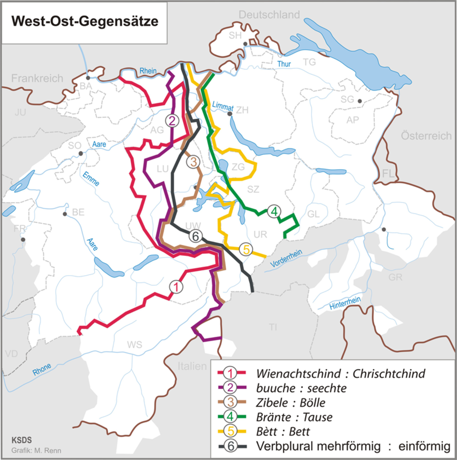
The Swiss dialects are most comprehensively documented in the SDS, which represents ca. 1,500 maps with 565 sites each.Footnote 1 This is thus the most relevant data source for Swiss dialects in the 20th century. Its author, Hotzenköcherle, as well as other scholars, tried to schematically classify the Swiss language area on the basis of SDS maps (see Kelle, Reference Kelle2001 for a discussion). The main aim was to identify regions with particularly similar language systems. In this context, the relevance of a primary east-west divide or a primary north-south divide of the spatial structure was a key question. Older literature stresses the north-south divide. In contrast, Hotzenköcherle himself (Reference Hotzenköcherle1984:51) emphasized the role of the east-west divide. More recent literature agrees with the drawing and quartering by Haas (Reference Haas, Bickel and Schläpfer2000:67), illustrating the relevance of both divides with the assumed primacy of the east-west divide. It has become clear from this literature that the spatial structure does not seem to be immediately visible. This leads to the impression that the dialects form part of a continuum, rather than a clearly defined categorical structure.
Nevertheless, the two divides are frequently used for linguistic orientation as, for example, in the atlas by Christen et al. (Reference Christen, Glaser and Friedli2019:32f.), who report a selection of isoglosses identified as markers for the two divides. These are reported in Map 1 and Map 2, which both demonstrate a distinct separation of the Swiss cantons. Most parts of Solothurn (SO), Basle (BA), Aargau (AG), Luzern (LU), Zurich (ZH), Schaffhausen (SH), Thurgau (TG), St Gallen (SG) and Appenzell (AP) clearly belong to the northern part. Valais (WS, abbreviated to VS in this study to avoid confusion with the Wenker sentences), Nidwalden (UW), Schwyz (SZ), Uri (UR), Glarus (GL) and Grisons (GR) belong to the southern part. BA, SO, AG, Fribourg (FR), Bern (BE) and VS belong to the western part; and SH, ZH, SZ, GL, GR, TG, SG and AP belong to the eastern part. Especially, Zug (ZG) and LU are in the transition zone between the divides.

Map 1. North-South divide in German-speaking Switzerland (Christen et al., Reference Christen, Glaser and Friedli2019:32).
Map 2. East-West divide in German-speaking Switzerland (Christen et al., Reference Christen, Glaser and Friedli2019:33).
More recently, some dialectometric studies were performed on the SDS with normalized data, which had been broadly cleaned to remove rare or unique variants. Interestingly, almost none of these studies sought to visualize the dialect continuum but instead focused on the separation of individual dialect areas, almost always in the form of hierarchical clusters. In this vein, Kelle (Reference Kelle2001) performed a hierarchical cluster analysis for 101 SDS sites using 170 linguistic maps with individual language phenomena. He found the east-west divide in the first step of his clustering, together with four other clusters in subsequent steps, which, in addition, contribute to a north-south divide. Overall, this finding tended to support the more qualitative approach by Haas (Reference Haas, Bickel and Schläpfer2000), but with an emphasis on the “typological weight” (Kelle, Reference Kelle2001:29; our translation) of the southwestern part (Bernese Alps and Valais). In this regard, it became obvious that the east-west divide is more precisely a contrast between northeast and southwest.
A more comprehensive dialectometric study based on another SDS sub-sample was performed by Goebl, Scherrer and Smečka (Reference Goebl, Scherrer, Smečka, Schneider-Wiejowski, Kellermeier-Rehbein and Haselhuber2013). The sample, which revisits analyses by Scherrer (Reference Scherrer2012; see also Scherrer & Kellerhals, Reference Scherrer and Kellerhals2014), covers ca. 200 maps (phenomena) with 565 sites each. The data have been largely normalized (e.g., in phonological terms but also in eliminating rare or unique variants) and evaluated with dialectometric techniques. As a result, the authors found clear structuring divided into different spatially coherent clusters. An interesting finding was, among others, that the splitting of clusters starts in the western area, where it continues from north to south. This is slightly different to the finding of Kelle (Reference Kelle2001), whose clusters continue from east to west. This could be due to different data selection, but is most likely to result from the different data fusion algorithms used by the authors. While Kelle (Reference Kelle2001) uses the complete linkage algorithm, Goebl et al. (Reference Goebl, Scherrer, Smečka, Schneider-Wiejowski, Kellermeier-Rehbein and Haselhuber2013) prefer the Ward algorithm.Footnote 2
The aim of Scherrer and Stoeckle (Reference Scherrer and Stoeckle2016) is to analyze different linguistic levels. To this end, they merge Scherrerʼs SDS sample with more recent data from the Syntaktischer Atlas der deutschen Schweiz (SADS) currently being processed. Here, too, the authors performed cluster analyses based on Wardʼs algorithm. Once again, the clustering of all data showed the divide from north-east to south-west, which continues, in this case, over three gradations in the first cluster steps. Finally, the north-south divide also became apparent. An interesting difference from the study by Goebl et al. (Reference Goebl, Scherrer, Smečka, Schneider-Wiejowski, Kellermeier-Rehbein and Haselhuber2013) is that the cluster steps follow another direction. Whether this is due to the impact of the merged syntactical data is still an open question. Additionally, the authors provide insights into the dialect continuum by discussing maps of average distance and some dispersion measures (standard deviation and skewness). All these measures highlight more or less coherent areas with higher or lower values, which indicates significant spatial structuring within the dialect continuum.
To the best of our knowledge, a study that directly relates the (unstructured) historical Wenker data to the SDS data using computational methods has not yet been performed.
3. Material and methods
3.1 Corpus
The Wenker corpus was initiated by the German linguist Georg Wenker between 1876 and 1888 (see Wenker, Reference Wenker2013). Wenker designed a questionnaire of 40 Standard German sentences, which he sent out to all the schools of the German Empire where pupils and teachers were asked to translate these sentences into their local dialect (see Chambers & Trudgill, Reference Chambers and Trudgill1998; Lameli, Reference Lameli, Auer and Schmidt2010, Reference Lameli2014). Wenker obtained a total of about 45,000 handwritten translations from this survey, which ultimately formed the basis of the renowned Sprachatlas des Deutschen Reichs (‘Linguistic Atlas of the German Empire’; see Reference Schmidt, Herrgen and KehreinREDE). From a geographic perspective, to this day, this atlas remains one of the most (if not the most) comprehensive record of German dialects, while, from a corpus linguistic perspective, the translations form one of the largest parallel corpora in dialectology.
However, since the survey only covered the area of the German Empire, subsequent surveys were conducted in neighboring German-speaking countries and areas. In Switzerland, questionnaires were sent out between 1933 and 1934 to 2,749 locations, of which 1,769 were returned (i.e., 64%). The quality of the Wenker material is a bone of contention. While Maurer (Reference Maurer1926:70) finds complete agreement (even in small details) between translation of the Wenker sentences and dialectal sources of that time, other authors take a dim view of the material (see Fleischer, Reference Fleischer, Christen, Gilles and Purschke2017b:141). At the time of Wenkerʼs study, it was mainly Bremer (Reference Bremer1895) who complained about the lack of validity of the data. However, more recent studies have demonstrated the validity of the data for dialectological analyses (see Schmidt & Herrgen, Reference Schmidt and Herrgen2011, for a discussion).
As with other regions, the phonetic accuracy of the Swiss data has also been questioned, leading to doubts about the value of the material. A more detailed answer to this question remains outstanding, but assessments of these data are available, such as that of Hotzenköcherle, one of the co-founders of the SDS, who considered the material to be “extremely valuable” in 1944 (see Fleischer, Reference Fleischer2017a:113f.). More recent studies have at least proved the syntactic value of the Swiss data (Kakhro, Reference Kakhro2005; Fleischer, Reference Fleischer and Huck2014, Reference Fleischer, Christen, Gilles and Purschke2017b). This is all the more remarkable when one considers that the questionnaire was not designed for syntactic issues. Against this background, there is some evidence that the data are underrated, which is why we consider a closer look to be more than appropriate.
On the basis of the digital edition of the Swiss questionnaires, which is available in raster format (scans) from the REDE platform at Marburg University (see Ganswindt, Kehrein & Lameli, Reference Ganswindt, Kehrein, Lameli, Kehrein, Lameli and Rabanus2015), we compiled the sample for the present study. Between 2014 and 2015, a subset of these questionnaires was transcribed into a machine-readable format by student assistants at Zurich University.Footnote 3 Their task was to reproduce all graphic information (characters, diacritics, etc.) from the originals. Since transcribing all 1,769 questionnaires would have been too costly and time-consuming, a sample was taken of sites which coincide with the SDS sites and those from the more recent syntactic atlas of German-speaking Switzerland (SADS). In addition, we randomly chose sites which ensured a preferably equal distribution of locations all over German-speaking Switzerland. In this way, a set of transcriptions of Wenker questionnaires was eventually obtained from 616 sites, which is 35% of all questionnaires.Footnote 4
3.2 Methods
3.2.1 Dataset and (non-)normalization
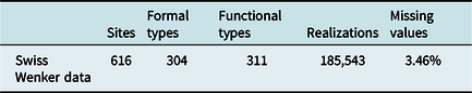
Further preparation and analyses were carried out at Freiburg University and Marburg University, respectively. All items have been semi-automatically aligned according to the Standard German stimulus (i.e., serialization of words is ignored), cleaned of punctuation and transformed into a lower-case representation. The original questionnaire contains 468 tokens, 311 functional types (types with one specific grammatical function each) and 304 formal types (i.e., homographs, e.g., <sind> for 1.pl.pres and 3.pl.pres; see below for further explanation). Theoretically, based on the number of functional types, there were more than 190,000 realizations across all 616 sites. However, largely due to some missed translations, this total cannot be reached in the actual corpus (see Table 1).
Table 1. Characteristics of the Swiss Wenker corpus
The difference in number of tokens and formal types is mainly due to high-frequency functional words, such as articles, pronouns, modal verbs or auxiliaries, while the difference between formal types and functional types is due to data preparation, which became necessary in the course of data alignment. By way of example, this procedure can be demonstrated with the auxiliary sind ‘are’, which is a homograph for 1.pl.pres and 3.pl.pres in Standard German. In the questionnaire, it is represented five times as 3.pl.pres (WS 6, 13, 2×29, 38) and once as 1.pl.pres (WS 23). The 3.pl.pres forms were represented as a single one because of the identical grammatical status and syntactic context. The formal type sind thus occurs as two functionals types in our corpus. This explains why the number of functional types is slightly higher than the number of formal types.
Furthermore, in order to reduce the number of missing values, every variable (i.e., the Standard German stimulus) was evaluated in terms of the consistency of its dialectal representations. An example is provided by WS 3: Tu Kohlen in den Ofen, damit die Milch bald an zu kochen fängt ‘Put coal into the stove so that the milk starts boiling soon’. Take the syntagma an zu kochen fängt ‘starts boiling’ in the final clause, which is a combination of a separable verb (an-fangen ‘start’), a particle (zu ‘to’) and an infinitive (kochen ‘boil’). At almost all sites, this is translated without the particle and with a non-separated variant of the type afot Ø inf (see Schallert & Schwalm, Reference Schallert, Schwalm, Alexandra and Patocka2015 for a broader discussion of the phenomenon). In our corpus, the items of the Standard German syntagma were hence compensated by only two Standard German variables, namely anfängt (‘start-3.sg.pres’) and kochen (‘boil-inf’), while the particle zu remained disregarded. In so doing, the number of missing values could be significantly reduced.
Aside from these two interventions, which concern standard language rather than the dialectal representation, the data were left in their original format because of the uncertain status of many realizations. This brings the normalization of dialect realizations into focus. Normalization means categorization of realizations provided by the dialect corpus.Footnote 5 Take, for example, the normalization of phonological items. Some studies only combine the nuances of certain allophones, while others combine larger groups of allophones. An example is provided in Figure 1, which is an extract from the SDS map of the verb bauen. In this example, particular nuances are classified according to the expertise of the dialectologist who designed the map. In contrast, for his SDS sample, Scherrer transferred this classification into larger classes, combining lines 1 and 2 to an ou type, and lines 3 to 5 to an au type. Even though this categorization is already indicated by the shape of the SDS symbols, the different degrees of detail illustrate that the normalization process is rather subjective in nature.
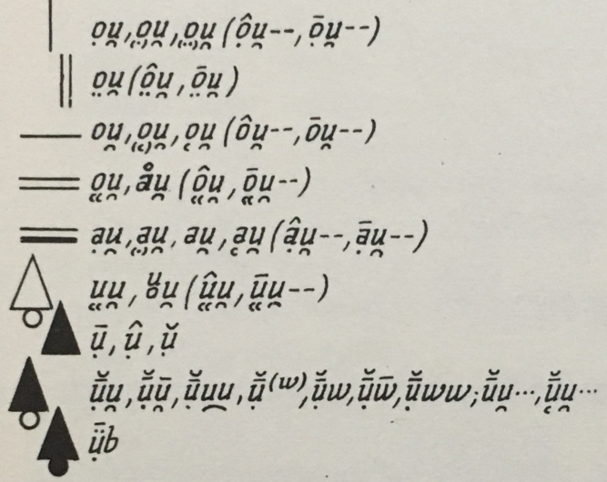
Figure 1. Extract from the legend of the SDS bauen map (vol. I), demonstrating the classification of phonetic variants.
Commonly, the frequency of individual variants serves as a criterion for combination. In some cases, rare or unique variants that are obviously functionally irrelevant or idiosyncratic are even excluded from analysis, as is the case with the original SDS maps, which were cleaned even further with the SDS sample provided by Scherrer. The main advantage of data normalization is the fact that pre-structured data enable a better overview of those items the map designer considers to be the functionally most important ones. Typically, this results in more clearly structured maps without any noise, which is why most language atlases (except for those in the Romance tradition) map only normalized data. In all cases, this advantage is at the expense of lower data objectivity (the SDS provides information on original forms in individual commentaries).
For the Wenker data, there are some cases where normalizing seems simple at first glance, whereas others are more complicated or even impossible. An example is provided by the relatively seldom-used realization <bleter> (‘leaf-pl’), in contrast to the most frequent <bletter>. In the German orthography, a short vowel quantity is often indicated by doubling the subsequent consonant, as in <Blätter>. Against this background, a single <t> could refer to a long quantity of the stem vowel. Indeed, a long quantity is documented in realizations such as <bleeter>, which is why normalization into this variant could make sense.
However, there could also be another explanation. Swiss dialects are known for the existence of geminates at syllable boundaries (Wiesinger, Reference Wiesinger, Besch, Knoop, Putschke and Wiegand1983:833). Consequently, <t> could also refer to the circumstance in this particular dialect where ‘leaf-pl’ comes without gemination (/t/ instead of /t.t/). In this case, <t> is not attributed to vowel quantity but to consonant quantity, which is why the realization should be preserved as it is. Against this background and without a deeper analysis, in this example, there can be no certainty as to what the <t> (rather than <tt>) is referring to. Any normalization into <t> or <tt> might, therefore, be misleading.
This is why normalization of the Wenker data is not only challenging but also risky.Footnote 6 It is thus not surprising that even Wenker himself always relied on the original variants when mapping his data and refrained from normalization. In view of the finely graded linguistic information that laymen sometimes put into their translations, decisions about which cases should be subjected to normalization and which cases should not, seem arbitrary. To avoid this problem, we follow Wenkerʼs procedure and take the data as they are—without normalization. This leaves us, however, with very noisy data which, in turn, is challenging from a methodological perspective. Instead of the normalization of raw data, we, therefore, make careful use of (spatial) classification techniques and nearest-neighbor smoothing functions, which are suited to capturing important geographical patterns ex post. This procedure is also not without problems. For example, smoothing could lead to real exceptions (e.g., language islands) becoming obscured. This is why we always present smoothed data together with original, non-smoothed data.
However, this procedure does not facilitate direct comparison of individual realizations of the Wenker sample and the SDS reference sample (see section 3.2.4). In order to evaluate the distribution of individual variants in these samples, we normalize a selection of linguistic variables from the Wenker data according to the procedure of the reference sample. This selection, which is based on realizations with a clear phonological status, is reported in section 4.1, together with further information on the normalization process.
3.2.2 Distance measure
In order to analyze the overall structure of Swiss dialects, different linguistic distance measures were performed. In this article, two approaches are reported based on Levenshtein distance.Footnote 7
The most straightforward approach is unweighted Levenshtein distance (LD; Levenshtein, Reference Levenshtein1966). LD is the minimum cost when transferring a string S 1 into a string S 2 under the consideration of substitutions of segments, as well as insertions and deletions. Actual costs are expressed as the number of these operations (so-called edit distance). In the case of the Wenker sample, this distance refers to graphotactic particularities, which intentionally (i.e., from the perspective of the transcribers) reflect phonological issues. More technically, comparison of two strings is a comparison of the linear set of characters i with the linear set of characters j. LD ij is then the edit distance of S 1, where 1 ≤ S 1 ≤ i and S 2 is 1 ≤ S 2 ≤ j. Calculating these distances pairwise for all 616 sites creates a 616×616 distance matrix D. The particular distances of this matrix are referred to as linguistic distances. With this measure, it becomes possible to find those areas which are, from a linguistic perspective, similar or different to a certain extent.
Furthermore, we perform a measure LD ϕ. Here, the frequency of tokens is calculated. Based on the individual sums per site, a weighting matrix F is constructed, which will be multiplied by the distance matrix D resulting from the LD measurement. This measure is conceptually similar to the GIW measure introduced by Goebl (Reference Goebl1984:76). In contrast to LD, LD ϕ not only calculates the phonetic differences in segments but, at the same time, weights frequent realizations more highly and less frequent realizations to a lesser extent. This procedure is suited to finding those areas where most typical realizations are dominant.
Finally, a remark on the treatment of synonyms is necessary. Once more, we refer to WS 3 above where, in some instances, the kochen ‘to boil’ variable is realized as the non-cognate sieden (etym., ‘to seethe’). As there is no discernable functional difference, we decided not to exclude synonyms in this example. The same holds true for the remaining variables of the corpus. As a consequence, LD between non-cognates might be larger than for cognates, but this obviously reflects, on the other hand, the actual language situation.
3.2.3 Data imputation
In total, our data show 6,655 missing values (3.46%), which equates to 10.77 missing values per site on average. Even though this is a rather small amount, it is, nevertheless, a considerable problem for the LD measurement. If there is no string available, transformation into another one is not possible. As a consequence, every site with missing translations is necessarily excluded from computation. However, as every site has missing translations in at least one of the variables, computation of the LD is no longer possible.
Our solution to this problem is to compensate for the missing values by average distances. In detail, we (1) defined missing translations as strings of zero length; then (2) performed the distance measure; (3) calculated for every variable the mean of non-missing sites; and (4) input this into the missing translation cells afterwards.
3.2.4 Reference sample
In order to validate our findings, the Wenker data have been related to the SDS data. The SDS data were gathered between 1939 and 1957, which is why the two samples represent similar periods. They contain, however, different linguistic items and data types.
For the purpose of a computational analysis, it is possible to use the digitized SDS sample provided by Scherrer (see Scherrer, Reference Scherrer2012, Reference Scherrer and Huck2014; Goebl et al., Reference Goebl, Scherrer, Smečka, Schneider-Wiejowski, Kellermeier-Rehbein and Haselhuber2013; Scherrer & Kellerhals, Reference Scherrer and Kellerhals2014; Scherrer & Stoeckle, Reference Scherrer and Stoeckle2016), although this only represents an extract of the SDS.Footnote 8 The sample provides normalized data which, in contrast to the Wenker corpus, result from oral interviews undertaken onsite by linguistically trained fieldworkers. The questionnaire items also differ to a large extent. According to Scherrer and Kellerhals (Reference Scherrer and Kellerhals2014), the SDS sample documents 234 linguistic items from phonology, morphology, and lexis, which are provided as individual segments (for example, phonemes or morphemes) or sequences of segments (for example, word endings).Footnote 9 Even though the original SDS data is more detailed in terms of data representation and interpretation (e.g., highlighting particular transcriptions, referring to uncommon realizations and sometimes reporting informants’ comments in the legends of the maps), Scherrerʼs sample comprehensively documents the core information of the individual maps. However, according to Scherrer and Stoeckle (Reference Scherrer and Stoeckle2016:96), the data have been reduced more extensively than was the case with the original SDS by very rare (and sometimes unique) variants, while variants which were difficult to distinguish have been merged. The sample thus represents a stronger degree of normalization and data cleaning than the original SDS maps do. Some further characteristics are provided in Table 2.
Table 2. Comparison of the Swiss Wenker corpus with the SDS sample provided by Scherrer (Reference Scherrer2012; see also Scherrer & Kellerhals, Reference Scherrer and Kellerhals2014)
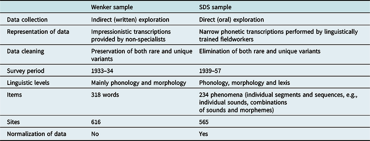
Table 2 makes it clear that the two corpora are comparable regarding the number of sites and linguistic items. The number of actual coincidences is, however, smaller. In total, there are 349 sites, which are represented in both samples. In terms of the representation of data, the two samples differ in a fundamental sense. Not least, normalization of the data and the handling of rare variants is an important difference between the samples.Footnote 10
3.2.5 Map correlation
In order to perform correlation analyses between the spatial distributions of individual lemmas of the Wenker and SDS samples, a quadratic counting approach has been used. In detail, for both the Wenker sample and SDS sample, we span a grid of 20×20 quadrants over the area of investigation, counting the number of variants inside every quadrant. Spearmanʼs rho is then calculated for every lemma of the samples.Footnote 11 In order to average the individual correlation coefficients, Fisherʼs z transformation is used. In so doing, we are able to evaluate the strength of the relationship between the two samples.
4. Data analysis
4.1 Individual phenomena
It has already been pointed out above that the overall linguistic value of the Swiss Wenker material is rather unclear. This is mainly due to the fact that only syntactic studies are available. Against this background, some insight into the data is provided by the following examples, which we consider to be rather typical ones: Map 3 shows the spatial distribution of graphic variants of the verb bauen (‘build-inf’, WS 33), the verb schneien (‘snow-inf’, WS 2) and the adjective früher (‘early-comp’, WS 15). Map 3/A–C maps the raw data of each word on the lexical scale. To capture the geographical patterns more effectively, Map 3/D–F provides a slight smoothing of these data, based on selection of the most frequent variant in the five nearest neighbors of each site.Footnote 12
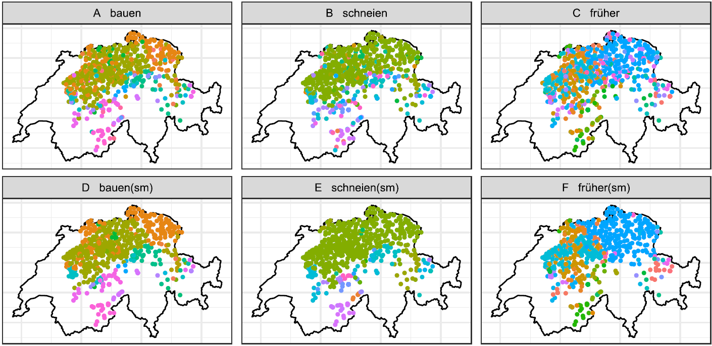
Map 3. Spatial distribution of selected realizations from the Wenker sample; A: bauen (‘build-inf’); B: schneien (‘snow-inf’); C: früher (‘early-comp’); D–F: smoothing of A–C data.
Despite the large number of individual realizations (bauen encompasses 48 different realizations, schneien = 64, and früher = 108), every map shows more or less coherent spatial patterns. These patterns are usually due to only four or five realizations, each forming part of at least 3% of all tokens (see Figure 2). The remaining tokens are typically unique variants (hapax legomena in the terminology of corpus linguistics), which is why the overall frequency distributions in the Wenker sample resemble a Zipfian distribution (see section 4.2.2).
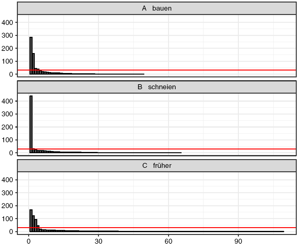
Figure 2. Statistical distribution of the realizations in Map 3 together with the 3% level of all realizations (red line).
In order to evaluate these maps more closely, each lemma must at least be roughly related to the corresponding lemma in the SDS sample. We will, therefore, deviate from our conception at this point and try to attribute the graphic realizations to identifiable sound types. To this end, both datasets are reduced to identical sites. As the SDS data only report extracts from the stimulus word (segments or sequences), which have also been normalized to particular types, the Wenker data should be arranged in the same way. As with the SDS, unique word representations were eliminated, relevant segments or sequences of remaining words were extracted, and comparable spellings merged (e.g., schneien stem vowels <i, î, j, y, ii, ij, iy, ji, yj> are classified as ii). Realizations that could not be unambiguously assigned were excluded as well as homonyms.
Bauen: Map 4 compares the normalized extract (stem vowel) from Map 3 with appropriate data from the SDS sample. Statistically, the two maps are moderately related (r(398) = .575, p < .001). There is a larger au region in the northeastern part; a larger ou region in the western part as well as in the central part; a larger region of uu variants in the Alpine region; and a smaller ui region in Central Switzerland (see Map 1 and Map 2 for a geographically more detailed description).

Map 4. Realizations of the stem vowel std. /![]() / in bauen (‘build-inf’) from the Wenker sample against the SDS sample.
/ in bauen (‘build-inf’) from the Wenker sample against the SDS sample.
Most interestingly, both maps indicate particular au occurrences within the ou region, which lead to a blurred picture. Evaluating the Wenker map alone could imply this heterogeneous pattern as a methodological artifact. However, since it is also provided by the SDS sample, it seems more likely that the maps reflect language variation. What is more, as the locations of the interfering dots differ between the maps, this indicates that local variation is higher than the samples individually suggest.
Another point could be addressed. Looking at the original SDS maps, the au variants in the central western part are missing to a large extent. However, as mentioned above, in his SDS sample, Scherrer merged the au variants with the phonetically most-closed ou variants, visualized with similar symbols in the SDS. In this respect, the Wenker data support Scherrerʼs normalization procedure (and the SDS-visualization), while Scherrerʼs procedure provides support for naïve discrimination of the sound continuum performed by Wenker data informants. At the same time, it should be emphasized that at least some of the au variants in the Wenker data might be influenced by written German, which has the au diphthong as well.
Against this background, comparison of these two maps reveals that the Wenker data, despite their noisiness, are able to capture complex structures in language geography. It is also clear that comparison of the two samples contributes to a more comprehensive interpretation of the linguistic phenomena under investigation.
Schneien: In the case of the schneien maps, the results are different. Map 5 documents four types of stem vowels. Among these, strong relations can be seen between the spatial distributions of ei (ρ(391) = .795, p < .001) and ii (ρ(391) = .867, p < .001) but not for ai, which is omitted from the Wenker sample, as is the e type in the SDS sample. On average, the relation between the two maps is thus not significant in statistical terms (r(391) = -.016, p = .752).

Map 5. Realizations of the stem vowel std. /![]() / in schneien (‘snow-inf’) from the Wenker sample against the SDS sample.
/ in schneien (‘snow-inf’) from the Wenker sample against the SDS sample.
In terms of linguistic quality, the SDS map seems to capture the linguistic scene more appropriately as it distinguishes the well-known difference between /![]() / and /
/ and /![]() /. Even though the Wenker data show clear spatial patterns, they do not successfully identify the ai region of the SDS sample. We can find at least one <schnaie> record in the western region among these sites, which does not correspond to the SDS sites.
/. Even though the Wenker data show clear spatial patterns, they do not successfully identify the ai region of the SDS sample. We can find at least one <schnaie> record in the western region among these sites, which does not correspond to the SDS sites.
This absence is likely due to the graphic representation of the Wenker data. In Standard German, <ei> represents /![]() /, whereas, as the SDS map indicates, in some Swiss dialects it represents /
/, whereas, as the SDS map indicates, in some Swiss dialects it represents /![]() / as well. As these /
/ as well. As these /![]() / diphthongs are not represented in spoken Standard German, there is consequently no grapheme available, which is why the Wenker informants use <ei> instead. Consequently, what may appear to be a unique area of <ei> graphemes, is in fact a mixture of different phoneme-grapheme correspondences.Footnote 13 In this example, the SDS sample thus helps to validate the Wenker data and, in so doing, reveals information about the non-specialists’ conceptualization of writing.
/ diphthongs are not represented in spoken Standard German, there is consequently no grapheme available, which is why the Wenker informants use <ei> instead. Consequently, what may appear to be a unique area of <ei> graphemes, is in fact a mixture of different phoneme-grapheme correspondences.Footnote 13 In this example, the SDS sample thus helps to validate the Wenker data and, in so doing, reveals information about the non-specialists’ conceptualization of writing.
Früher: Another observation is offered by the früher maps, which demonstrate a moderate correlation (r(290) = .452, p < .001). Here, we find a rather blurred picture for the Wenker sample and a clear structuring of the SDS sample. While the SDS sample only reports variation in word endings, the Wenker map also shows lexical variation in terms of the differentiation of a früher type vs. an eher type. That these eher realizations are, however, not incidental, is underlined by the clear regional pattern, which is best highlighted in Map 3/C and Map 3/F.
This seems to be due to the syntactical context. In Standard German, früher is an ambiguous form of the adjective früh for both nom.sg.m and comp, as with many dialects. While the SDS focuses on the former in an attributive position (ein früher Winter ‘an early-nom.sg.m winter’), the Wenker questionnaire focuses on the latter in an adverbial position (darfst früher heim gehen ‘may go home early-comp’). As Map 6 illustrates, the formal congruency is typical for the eastern part of Switzerland, whereas the western part at least partially disambiguates meanings by using the eher variant in the adverbial position. In this case, comparison of both samples again contributes to a more comprehensive interpretation of the linguistic scene. While in the bauen map the phonetically more precise SDS data helped to validate the impressionistic Wenker data, here, the Wenker data help to grammatically specify the SDS data, indicating the partial restriction of the früher form to an attributive position.

Map 6. Realizations of früher (‘early-comp’) from the Wenker sample against the SDS sample.
Map 6 is also interesting, however, from a more methodological perspective. If there were only Map 6/A, which is based on the reduced sample, the clear spatial pattern of the eher type would be hard to realize, if at all. This differentiation is made clearer by the more comprehensive sample in Map 3/C and especially in the smoothed version of Map 3/F. This increase of data quality through increased data quantity is exactly what Wrede (Reference Wrede, Wenker and Wrede1895) had already found with the more historical Wenker data.
4.2 Aggregation of the Wenker data
4.2.1 Spatial patterns
This section considers the level of data aggregation. In contrast to the previous procedure, we consider both the non-normalized, word-based representation of raw data and all other sites, which are not represented in the SDS sample.
The Wenker data were initially evaluated in terms of spatial patterns using a technique introduced by Heeringa (Reference Heeringa2004), focusing on visualization of the continuity of data via the transformation of multidimensional scaling (MDS) coordinates into RGB color space. Map 7/A plots these vectors in geographical space. In order to sharpen this picture slightly, Map 7/B presents a smoothing based on the three nearest neighbors. For both maps, similar colors refer to small linguistic distance between the sites; different colors refer to large linguistic distance between the sites. The maps thus (1) highlight the linguistic differences as such and (2) allow statements about the degree of linguistic distance between the sites.

Map 7. Linguistic distance between Swiss-German sites; A: MDS plot of unweighted data (three dimensions in RGB color space); B: nearest-neighbor smoothing of A (three neighbors).
The two maps illustrate a spatial continuum together with some striking areal concentrations. The most different regions are the northeastern part vs. the southwestern part, and the northwestern part vs. the southeastern part. This situation is due to three prominent axes within the continuum. There is (1) a continuum on an axis from east to west; (2) a continuum in the east from north to south; and (3) a continuum in the west from north to south. The latter shows a clearer subdivision than the eastern one does. The regions around Freiburg/Uechtland, the Bernese Alps and the Valais are most prominently separated (FR, the southern part of BE and WS in Map 2). Altogether, this is a structuring, which is in line with the related literature (e.g., Kelle, Reference Kelle2001; Scherrer & Stoeckle, Reference Scherrer and Stoeckle2016). It thus reveals evidence for the reliability of the unstructured Wenker data.
4.2.2 Frequency of tokens
A region such as the Valais, which occurs as a clear but small area in Map 7, is highly likely to be characterized by rather rare variants. This is confirmed by all existing literature. However, the extent of the effect on the remaining spatial pattern caused by the frequency of all other realizations is not clear. Against this background, this section is dedicated to the impact of token frequency on spatial structuring. As an initial approximation, Figure 3/A shows the frequency of all tokens of the Wenker corpus against their frequency rank. Obviously, there are only a small number of tokens with a very high frequency, and most tokens are either rare or unique ones. The highly right-skewed pattern resembles a Zipfian distribution, which is the typical one for corpus data. More precisely, the log-log plot in Figure 3/B indicates a broken power law consisting of at least two Zipfian sections (indicated by the break around rank 200 in Figure 3/B), each approximating a lognormal distribution, as Figure 3/C and Figure 3/D demonstrate.Footnote 14

Figure 3. Token frequency in the Wenker sample against the frequency rank of tokens; A: overall pattern; B: log-log plot of frequency distribution against fitted power law (red) and lognormal distribution (blue); C: same as B for rank one to 200; D: same as B for rank 201 to 11,807.
Figure 3 indicates not only significant differences between the tokens but also a large quantity of unique, or at least rare, variants, constitutive for the noisiness of our data (see Figure 2). At the same time, the circumstance of there being more than one Zipfian distribution raises the question of whether these differences are due to particular spatial structuring. Using the LD ϕ measure, we tried to get evidence for this assumption.
However, implementation of this requires a short reflection on the spatial distribution of sample points. Given a disproportionately high number of sites within a region, the variants of these regions, as a consequence, are disproportionately frequent in the sample. A random sample (like the Wenker sample) is typically not balanced in terms of the spatial distance between neighboring sites. Consequently, it is highly likely that there are clusters of sites which are biasing the results. This is exactly what happens when performing LD ϕ on the overall sample.Footnote 15
It is thus necessary to balance the sample by a more regular arrangement of sites. To this end, we span a quadratic grid of 1,000 reference points over the area under investigation and choose the sites closest to each reference point as representatives in the new sample. This produces a non-clustered sample of 392 sites (instead of 616), which serves, for our corpus, as the most suitable input for the LD ϕ measure. Map 8 provides the result of this measurement. For a better evaluation of the degrees of frequency, LD ϕ was transformed into 0 > LD ϕ > 1, where 0 (indicated by the color purple in Map 8) refers to regions where tokens of the lowest frequency occur, and 1 (shown in red) refers to regions where tokens of the highest frequency occur.Footnote 16

Map 8. Distribution of most frequent tokens in the spatially balanced extract of the Wenker sample (N = 392 sites) based on LD ϕ measure.
Map 8 shows a very clear spatial dependency of token frequency. The red region describes the largest possible intersection of all realizations of our corpus. That is, the realizations of this region have a particularly high typicity of Swiss-German dialects. The purple region, on the other hand, has the smallest intersection of realizations and thus refers to a region in which realizations of particularly low typicity occur. Considering the previous maps, it is not surprising that these less frequent realizations occur in the Valais (WS in Map 1 and Map 2).
More striking is the spatial cluster of highest frequency in the center of the map, which is close to the city of Luzern (LU in Map 1 and Map 2). This region almost perfectly fits with the non-alpine part of the canton of Luzern. From there, a continuous decrease can be seen into the Alpine region and across the Alps, while the sites of the Swiss plateau form a more coherent picture. Against this background, Map 8 demonstrates a north-south divide with the region around Luzern as the center. This is exactly the culmination point of the two divides previously seen in Map 1 and Map 2. From these results, it must be concluded that this culmination point is a region of linguistic convergence characterized by the participation of variants of particularly high spatial coverage, i.e., communicative reach.Footnote 17
4.2.3 Classification
With the maps above, the question arises of whether it is possible to computationally verify the areal patterns as discriminable classes. For this undertaking, Kelleʼs (Reference Kelle2001) dialectometric finding of both an east-west and north-south divide, which is in line with the qualitative approach by Haas (Reference Haas, Bickel and Schläpfer2000:67), provides a clear expectation. To some extent, it has already been fulfilled in the description above. Starting from the assumption that coherent clusters can also be found in the Wenker data, we perform density-based clustering of the unweighted LD distance matrix using the DBSCAN measure (Ester et al., Reference Ester, Kriegel, Sander, Xu, Simoudis, Han and Fayyad1996).Footnote 18 In contrast to other clustering techniques, DBSCAN is not sensitive to noise as long as there are compact clusters in the data. However, as the previous figures indicate, this is not clearly the case. Consequently, as Map 9 shows, the result is rather unsatisfying when DBSCAN is based on the distance matrix (Map 9/A). Although clustering the northern part, DBSCAN does not succeed in clustering the south of the language area. Noise effects are predominate in the south in particular but also in parts of the northeast. Obviously, the data in these regions are too heterogeneous for clear clustering. However, this effect is dramatically reduced if the MDS data is used for pre-structuring. Then, DBSCAN reveals a coherent clustering (Map 9/B), which corresponds to the literature in terms of separating the east-west divide. The north-south divide is most of all visible in the eastern part of the map, where the Valais forms an area of its own.

Map 9. DBSCAN clustering; A: clustering based on unweighted distance matrix (color = clusters, gray = noise); B: clustering based on MDS data.
Since this is a very rough clustering (which was also achieved by pre-structuring the data), it raises the question of how a more precise clustering might be achieved. Therefore, like Kelle (Reference Kelle2001) and other related studies (e.g., Scherrer & Stoeckle, Reference Scherrer and Stoeckle2016), we also performed hierarchical clustering of the language area under investigation. The classification is again based on the unweighted LD measure; that is, we no longer use the pre-structured data from Map 9/B. In order to obtain the best fit between the clustered output data and the non-clustered input data, we follow Lameli (Reference Lameli2013:182) in measuring the cophenetic correlation between the classification result and LD measure using a Mantel test. The best fit after 1,000 replications is provided by the UPGMA algorithm (r(190,651) = .863, p < .001).
However, as Figure 4 demonstrates, UPGMA reveals a chaining effect, which means that this algorithm did not find larger clusters as did the DBSCAN algorithm in Map 9/A.Footnote 19 This is, at first glance, somewhat surprising from a methodological point of view as UPGMA is a conservative technique, which focuses on the average difference between clusters and thus typically does not generate chaining effects as does, for example, the more contractive single linkage algorithm. Considering Figure 2, it is highly likely that this effect is due to the large number of rare variants and hapax legomena, respectively. In normalized data, these phenomena are commonly eliminated to a large extent, which usually leads to more distinct clusters.

Figure 4. Dendrogram of UPGMA classification.
But this is all the more interesting from a linguistic perspective. It seems, in a way, that every site forms a more or less unique variety with only small indications for larger groupings. It thus seems appropriate to make use of another classification algorithm which, in contrast to UPGMA and DBSCAN, aims to minimize the within-cluster variance. We thus alternatively performed Wardʼs (Reference Ward1963) algorithm, which fulfills this specification. In fact, this technique reveals a very clear and spatially coherent clustering, demonstrated in Map 10.

Map 10. Areal classification of data following Wardʼs algorithm.
Even though this approach reveals a smaller cophenetic correlation (r(190,651) = .475, p < .001), it obviously provides a very coherent partitioning. Additionally, this clustering is in line with expectations from previous studies. For example, Map 10/A corresponds to the first step of partitioning found by Kelle (Reference Kelle2001:24). All other clusters found by Kelle are also included in Map 10, though these are on other levels of the clustering hierarchy and sometimes have slightly differing borders.
In the previous analyses, techniques of non-spatial classification were applied to data subject to an obvious spatial order. In order to take greater account of these spatial conditions in the classification, we make use of the so-called “first law of geography”, which is based on the idea that “everything is related to everything else, but near things are more related than distant things” (Tobler, Reference Tobler1970:236). That is, from a dialectological perspective, nearby sites are linguistically more similar than distant ones (Nerbonne & Kleiweg, Reference Nerbonne and Kleiweg2007). To this end, we added spatial information to the Ward clustering by including spatial constraints as provided by Chavent et al. (Reference Chavent, Kuentz-Simonet, Labenne and Saracco2017). We calculated a geographical distance weight ω = log(d), where d is the Euclidean distance between the sites. In order to keep the dominance of the linguistic information, we chose a conservative mixing parameter of α = .3, where 0 ≤ α ≤ 1. Technically, this means that sites from the first Ward clustering, which are not clearly attributed to one cluster or the other, are (in a second clustering step) weighted according to their spatial relations. This weighting is then decisive for the classification with nearby sites being weighted more highly and distant sites less so. Replicating Map 10/F thereby reveals Map 11/A. In addition, the eight clusters solution is also reported in Map 11, which reveals the most coherent clusters (Map 11/B).Footnote 20

Map 11. Spatial clustering of the Wenker data based on weighted Ward-like clustering; A: seven-cluster solution; B: eight cluster solution.
Overall, the differences between Map 10/F and Map 11/A are rather small. They mostly affect the heterogenous region in the northern part of the map, which fits fairly well with the canton of Aargau. Comparing the clustering in Map 11/B with the clustering of Goebl et al. (Reference Goebl, Scherrer, Smečka, Schneider-Wiejowski, Kellermeier-Rehbein and Haselhuber2013), which is also based on Wardʼs (non-spatial) algorithm, reveals a strong correspondence. In particular, the western part of the language area is quasi-identical, which becomes apparent, e.g., by the typical clustering of the region around Fribourg/Uechtland together with the Bernese Alps (indicated by a brown color in Map 11/B). However, there are also correspondences in the eastern part, which lead to the conclusion that, even though this study focuses on non-normalized and unstructured data, our analyses succeed in revealing a categorical structuring of the known Swiss-German language area which is in line with the existing literature.
4.2.4 Comparison with the SDS sample
In section 4.1, data from the Wenker sample were related to the largest comparable digital SDS sample available. As pointed out in section 1, Switzerland is the only country where it is possible to perform a data-driven comparison of Wenker data and narrower data by trained fieldworkers. Against this background, comparison with the SDS is of particular methodological interest as it is also important for analysis of other language areas. As the SDS sample comes without rare or unique realizations and, at the same time, provides normalized data, it might be assumed that the spatial analysis would reveal different results. However, as demonstrated in the previous sections, the spatial structuring of the Wenker sample is validated by the literature. We therefore additionally report the results of correlation analyses for the distance measures in this section. As the SDS sample is composed of binary indicator variables, it is not possible to apply the LD measure, which is why the Euclidean distance is calculated instead.Footnote 21 Similarly, a comparison between the LD ϕ measure is not possible as the SDS sample is not focused on words but on segments or combinations of segments.
Figure 5/A provides a closer look at the correlation between the two distance matrices. The distribution roughly resembles a logarithmic function. This is underlined by the non-linear regression curve (shown in red), which fits better with the data than does the linear one (shown in blue). The log transformation of the Wenker data in Figure 5/B hence effectuates the convergence of the two fits. Consequently, there is a fairly strong correlation between the datasets, which is slightly higher for the log-Wenker data (r(60,724) = .520, p < .001) than for the linear one (r(60,724) = .500, p < .001).

Figure 5. Wenker sample against SDS sample; A: matrix correlation with linear fit (blue) and non-linear fit (red); B: matrix correlation with log-Wenker data.
Regardless of whether a linear or non-linear relationship is assumed, it is remarkable that there is a fairly strong correlation at all given the extremely different datasets. This shows that despite all the heterogeneity, the Wenker data not only capture complex spatial structures at the level of individual phenomena (see section 4.1) but also at the aggregate level.
In terms of spatial structuring, this finding can be specified by considering the MDS coordinates. As a counterpoint to the comprehensive matrix correlation, we also calculate correlation of the matrix reduction in three dimensions, which reveals a similar result (r(1054) = .437, p < .001). However, when reducing the data into only one dimension, the correlation increases strongly (r(350) = .934, p < .001). The one-dimensional reduction is interesting from the perspective that it obviously captures the most prominent characteristics (i.e., more frequent realizations) of the sample, as Map 12 indicates, whereas it ignores the less frequent realizations. In this case, the east-west divide in particular is clearly separated, which has been the first step in the Ward clustering in Map 10/A.

Map 12. Comparison of one-dimensional MDS coordinates between the Wenker sample (A) and the SDS sample (B).
It is clear from Map 12 that the SDS sample tends to separate regions more clearly, which is to be expected if one considers that the SDS sample is focused on smaller types (e.g., word stems, morphemes, and vowels) with less variation than is provided by the representation of words in the Wenker sample. Nevertheless, considering that the Wenker data are (in contrast to the SDS data) unstructured and non-normalized, this comparison proves the fundamental suitability of the Wenker material for spatial analyses at the aggregate level. As no other studies have performed similar analyses for other language areas, this finding provides an indication of the representativeness of Wenker data in other regions.
5. Discussion
In this study, exploration of the Wenker data focuses on two main aspects: the spatial distribution of individual realizations and overall spatial structure of Swiss-German dialects. These points will now be discussed separately. Additionally, in terms of smoothing and clustering, we discuss some more general methodological issues.
5.1 Individual realizations
Among dialectologists of the 20th century, there was uncertainty about the validity of the Swiss Wenker data. As the data were provided by non-specialists using non-standardized transcriptions, it was unclear whether the data (with their enormous heterogeneity) could be considered at all representative of dialects. These concerns (together with the fact that the following SDS project provided data analyzed by specialists) were the main reason why the Wenker data remained unevaluated and, finally, sank into oblivion. In view of this background, comparison of the data with the SDS is most welcome—a comparison that is not possible with any other Wenker corpus in this way. It is interesting to see that the Wenker data gain important external validation through the data comparison, which was obvious from the schneien map (Map 5). However, this validation goes in two directions. A good example is provided by the bauen map (Map 4). Because of its apparent lack of systematics, if only the Wenker map was observed, the distribution heterogeneity would quickly give the impression that the representation was unreliable. However, the contrary is true, which becomes clear from a closer look at the corresponding SDS map. This map confirms that the Wenker material describes actual existing language variation. Comparison of the two partially different distributions, however, makes it clear that at that time more variation would be expected than the SDS alone could capture. In this regard, the Wenker material is an important addition to the simultaneously explored SDS. As most dialectological work of the 20th century is based on only very small groups of informants per location, this is undoubtedly a relevant finding for many other atlases as well.
From a more methodological perspective, it is obvious that the Wenker data offer a huge amount of hapax legomena, which are due to individual writing preferences and essentially contribute to the noisiness of the data. However, it is also clear that there are individual realizations, which are suited to revealing prominent spatial patterns of linguistic information. In some cases, these patterns are in accordance with the patterns of the reference sample, but in others they are not. In the maps presented above, these prominent realizations have a frequency of > 3% of the whole distribution of variants. In order to minimize the map complexity, one could consider eliminating the less frequent realizations (< 3%), but this would be inappropriate as some of these less common realizations are typical of regions with a minor impact on the overall distribution, such as the realizations of the Valais. The only way to deal with this variation is, from our perspective, to keep the different writing patterns and, if necessary, to smooth the variation ex post, e.g., by a conservative nearest-neighbor approach.
Furthermore, it has been obvious that the large number of sites is an important asset of the Wenker data. This becomes clear, e.g., by the früher maps. The reduction of data according to the SDS grid (Map 6) obscures to some extent the spatial pattern of the eher variant, whereas it is obvious in the larger sample (Map 3). It would, therefore, be highly desirable to digitize the remaining questionnaires as well.Footnote 22
5.2 Overall structure
First and foremost, finding that the unstructured Wenker data replicates well-known spatial structuring of Swiss-German dialects is an unexpected result, as discussed earlier. Given that all other dialectometric work dealing with the Wenker data relied on normalization of the original writings (e.g., Hummel, Reference Hummel1993; Lameli, Reference Lameli2013), this is the first time this result has become obvious.
Furthermore, our results imply that the relation of Swiss-German dialects (as represented by the Wenker data) is best described by the concept of a dialect continuum with particular concentration points (Map 7). This continuum, along with the strong similarity between dialects (some exceptions aside), might be the reason why the classification of Swiss dialects has been so difficult in the past (Haas, Reference Haas, Bickel and Schläpfer2000:60). This is best highlighted by Kelleʼs comment indicating surprise about the fact that despite “plenty of studies” (Kelle Reference Kelle2001:11; our translation), an accepted, more detailed spatial classification of Swiss-German dialects has not been possible before his study.
Certain areas of particular coherence showed up, which, due to the noisiness of the data, were hard to capture. However, in accordance with previous studies, our analysis demonstrated that on most maps the divide from (north-)east to (south-)west is the most characteristic one. It could be added that this divide, in accordance with the findings of Kelle (Reference Kelle2001), and Scherrer and Stoeckle (Reference Scherrer and Stoeckle2016), corresponds strongly with the so-called “Brünig-Napf-Reuss-Linie.” This border is one of the most prominent markers of the language areas in German-speaking Switzerland, which, at the same time, roughly coincides with former political boundaries. More generally, it was also identified as a relevant cultural border in earlier times (Weiss, Reference Weiss1947).
There is also, however, the north-south divide, which is commonly represented on the maps. As demonstrated, the intersection of the two divides, as it has been identified by Haas (Reference Haas, Bickel and Schläpfer2000:67) and Christen et al (Reference Christen, Glaser and Friedli2019:32f.; see Map 1 and Map 2 above), is fairly close to the region of the most frequent realizations (Map 8). We thus concluded that this culmination point is a region with variants of particularly high communicative reach.
From a methodological perspective, the MDS approach proved, in our context, to be the most powerful structuring technique. In order to derive clusters from the original distance matrix, hierarchical clustering techniques have been shown to be best suited to the noisy data under discussion, focusing on minimization of the within-cluster variance (Ward clustering and Ward-like clustering). Compared to the non-classified MDS coordinates, they show reasonably robust structuring. In our context, this is also an advantage over density-based clustering, which reveals more informative results when the data are pre-structured by MDS.
Finally, the connection with the SDS corpus should be mentioned, which reveals a fairly strong correlation based on the unstructured data and a very strong correlation based on the pre-structured data. Again, it must be highlighted that the two corpora differ in both the selection and representation of data. We conclude from this that the Swiss Wenker data not only provide a supplement to (and are partially corrective of) the SDS results in terms of local variation and grammatical refinement, but are also a very good reference point for the linguistic situation relating to German dialects in the first half of the 20th century.
5.3 Methodological reflection
The main challenge of this study in terms of revealing significant geo-linguistic information, was how to deal with the heterogeneity of the data. In contrast to nearly all other studies in the field, our approach was to avoid normalization and thus maintain data heterogeneity. Rare and unique variants were also considered, which are typically removed by linguistic atlases, at least to a large extent. This procedure was necessary because the data are difficult and, in some instances, impossible to normalize linguistically, as has been pointed out in section 3.2.1. Nevertheless, to reveal clear spatial patterns, we made use of (spatial) classification techniques and nearest-neighbor smoothing functions.
With regard to smoothing techniques, as highlighted in section 3.2.1, there were problems in terms of the obscuring of geographically isolated variants. However, as shown in sections 4.1 and 5.1, smoothing is a useful technique for reducing data heterogeneity, which obviates the need to simply clean up data by rare variants. Application of a conservative smoothing algorithm has, therefore, been key in this study (< 5 neighbors).
In terms of clustering, we have deliberately demonstrated techniques that were only partially successful. This makes it clear that the noisy data in question can be successfully processed, in particular, using techniques that aim to minimize within-cluster variance, as does the Ward algorithm (see sections 4.2.3 and 5.2). As has also been demonstrated, spatial weighting improves the classification result.
However, the question arises as to whether clusters are even necessary for linguistic description since it is stressed that a continuum is better for describing the language situation in German-speaking Switzerland. Clusters and hierarchies are not only necessary because they have enabled particularly good comparisons in existing studies, but in addition, they indicate (more factually) areas of concentration within a continuum. However, as the cophenetic correlation has shown, this was only possible by distorting the input data. This distortion mainly corresponds to the data cleaning caused by normalization in existing studies since the clustering of the Wenker data is consistent with these. Similar holds for the MDS mapping, where the one-dimensional MDS, in particular, leads to structural coincidence with the traditional data due to the higher weighting of more frequent realizations (r = .934).
All in all, this proves that complex spatial structuring can also be captured ex post on the basis of the noisy Wenker data. The main advantage of the approach presented here is that the actual heterogeneity of the data remains accessible and can be taken into account in later stages of the analysis. It should also be noted that the methods used here are not without alternatives. Depending on the corpus, other distance measures (e.g., n-grams), or classification approaches (e.g., machine learning techniques) may also be successful. However, for the corpus under discussion, the presented techniques were the most powerful.
6. Conclusion
In this article, we have presented a dataset containing Swiss-German Wenker sentences, provided by non-specialists between 1933 and 1934, including ca. 1,800 German local dialects. The data are noisy due to non-standardized phonetic transcription and have not yet been comprehensively analyzed, which is why we aimed to find evidence for the linguistic significance of the data. Using the previously digitized data, a large sub-sample of the Wenker corpus was compared to a sub-sample from the atlas of German-speaking Switzerland (SDS), realized by trained transcribers. Even though the structured SDS sample and unstructured Wenker sample differ fundamentally in their data representation, we successfully reproduced SDS information from the Wenker data. Similarly, we demonstrated a high level of correspondences in the overall spatial structuring of the two samples, even though the samples also differ in terms of data selection (r = 0.5 based on distance matrices; r = 0.9 based on an MDS vector). We concluded from this that despite the noisiness, the Swiss Wenker data are very well suited to capturing even complex structures in language geography and thus are very well suited to more detailed linguistic analyses than previously assumed. Against this background, this study is a promising starting point for exploration of the remaining parts of German-speaking Europe (in excess of 50,000 sites) represented by other Wenker corpora.
Acknowledgements
This research is supported by the Swiss National Science foundation (grants CR12I1_140716/1 and CR12I1_162760), the University Research Priority Program Language and Space (Zurich), the Academy of Science and Literature Mainz (grant REDE 0404) and the Research Centre Deutscher Sprachatlas (Marburg). We are grateful to Yves Scherrer for providing us with the SDS data and Jürg Fleischer for a selection of his already transcribed Swiss Wenker sentences. We are also grateful to two anonymous reviewers and the editors of the Journal of Linguistic Geography for their very helpful comments. Thanks also go to the auditorium of the 19th conference on Alemannic dialectology (2018) in Freiburg/Breisgau for vital discussion.


 Open access