


INTRODUCTION
In Argentina, bovine leukaemia virus (BLV) infection is common in dairy herds. In some areas (and especially in the Central Milk Region of Santa Fe Province) the proportion of infected herds is high (∼80%) and the within-herd prevalence ranges approximately from 40% to 50% [Reference Ghezzi1, Reference Trono2]. Currently, Argentina has a National Voluntary Control Programme (SENASA, 1994) but relatively few farms have enrolled. However, there is an increased interest of authorities and farmers to implement regional compulsory programmes but there is scarce quantitative information of the transmission of BLV in cattle herds which is needed to develop effective BLV control strategies.
The virus can spread by both natural and iatrogenic vectors that transfer blood (lymphocytes) from infected to non-infected animals [Reference Ferrer3]. Vertical transmission of BLV may occur post-natally through milk, colostrum, and by dam-to-calf contact and some calves born to BLV-infected dams will already have been infected in utero [Reference Piper4].
To develop successful interventions and to assign resources effectively, it is essential to understand the dynamics of the transmission and to have quantitative information of factors related to it [Reference De Jong5]. Mathematical modelling offers ways of integrating population level knowledge and epidemiological data to predict the outcomes of intervention scenarios. Deterministic models are commonly used for describing epidemics and are suitable when population sizes are relatively large. However, they are less suitable to simulate epidemics in relatively small populations, like within dairy herds, because disease transmission is fundamentally a stochastic process [Reference Diekmann and Heesterbeek6]. For small population sizes differences between individuals and random effects are important and stochastic models are needed to describe such situations.
One of the fundamental questions of mathematical modelling is to find threshold conditions that determine whether or not an infectious disease will spread in a susceptible population when the disease is introduced into it. The threshold conditions are characterized by the so- called reproduction ratio (R 0) [Reference Anderson and May7] a dimensionless parameter which encapsulates the biological details of different transmission mechanisms, such that if R 0<1, the modelled infection goes extinct, and if R 0>1, the infection may spread in the population. Due to the stochastic nature of the infection process there will be some probability that minor outbreaks will take place and infection will go extinct by chance. In our previous study [Reference Monti, Frankena and De Jong8], using data obtained from an observational study we estimated the value of R 0 as 8·8.
The purpose of the current paper is to gain an understanding of the dynamics of BLV transmission in dairy herds from Argentina by simulation and to compare various BLV transmission models and select the one that is most appropriate. Such a model can serve as a tool to evaluate the effect of several control strategies on the dynamics of transmission.
MATERIAL AND METHODS
Initial model overview and description of infection process
The hypothetical herd is conceptually described in terms of BLV status as a population of individuals that are protected by maternal antibodies (M), that are susceptible (S), that are in the latent period (E) or that are infectious (I). BLV is spread by contact between infected and susceptible individuals (horizontal transmission) and by infected dams giving birth to infected newborn calves (vertical transmission). Both types of transmission depend on the size of the susceptible subpopulation and transmission parameter β. The transmission parameter represents the probability per unit of time that a contact between an infectious individual with a susceptible one will result in the infection of the latter. In addition, once an animal becomes infected it remains infected for life and it will always be a potential source of infection [Reference Miller, Van der Maaten, Dinter and Morein9].
Population structure
We used an age-structured population model because disease can be transmitted either horizontally or vertically and infected animals remain a source of infection for the rest of their lives. Therefore, it is important to account for demographic changes in the population, for example, the rate of culling and the frequency of calving. In dairy herds, animals are usually kept in several age categories to optimize and facilitate management. Therefore, the population is heterogeneous and different contact patterns could be associated with different age groups.
In a standard management practice, representing a ‘typical’ farm of the area, the age groups can be defined as:
Group 1 (calves): includes all females from birth until 180 days of life.
Group 2 (heifers): includes all females from 181 days until introduction into the adult category (2 months before the expected date of calving).
Group 3 (adults): includes all pregnant heifers within 2 months of calving and all cows (dry, maternity and lactating).
It is assumed that groups are kept separately and no mixing occurs between groups while homogeneous random mixing occurs within groups. It is also assumed that the herd is closed and new animals enter by birth only, animals leave the herd due to sale or death. The hypothetical herd consisted only of females because in dairy enterprises male calves are either sold after birth or if reared they are moved to another production unit independent from the females.
Model selection
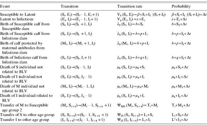
A scheme of the initial model is presented in Figure 1. The resulting model (MSEI) was used as reference and then compared with simpler models (that did not include some of the assumptions) to evaluate efficiency. Within-herd transmission was simulated by Monte Carlo techniques and Table 1 describes all events and their probabilities that were considered. We choose the smallest time-scale (12 h) (which is related to transmission of disease) because in our model we include two biological processes (disease transmission and demographic changes) that have very different time dynamics. The chance of a simultaneous jump of two events (neither related to disease transmission nor demographic) was sufficiently low to be neglected (1×10⁶) and we simulated a total time-horizon of 30 years.
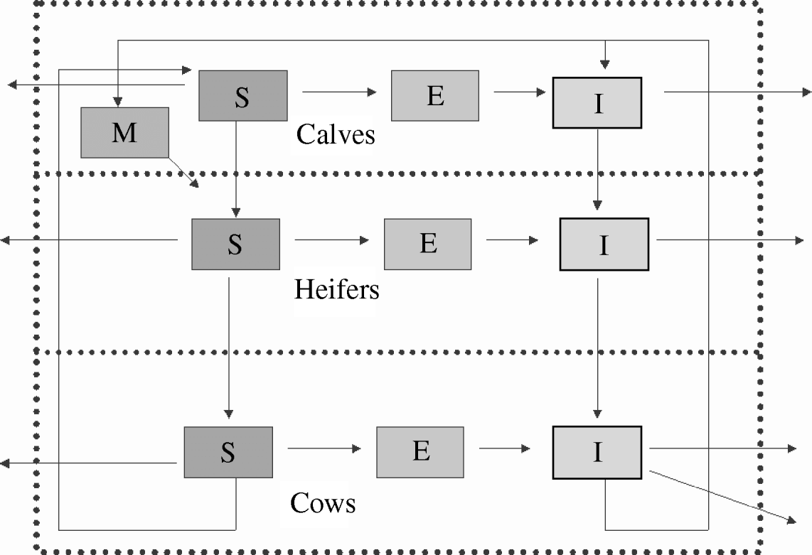
Fig. 1. A three-age-group model, showing the routes within compartments. The external bound represents the limits of the farm. M, Calves with maternal antibodies; S, susceptibles; E, animals in latent period; I, infectious animals.
Table 1. Description of possible events occurring in the MSEI stochastic model
The first step was to evaluate two aspects of the disease dynamics to decide whether or not they should be included in the model:
(1) the time-delay induced by the latent period (i.e. the period from where the animal got infected to when it became infectious, status E);
(2) the temporal immunity acquired by calves born from infected cows through passive transfer of antibodies.
When a virus is introduced in a naive population there will be few infective animals for a certain period, hence demographic stochasticity could lead to extinction of the infective agent. The probability of such extinction is defined as the probability of a minor outbreak (P minor). However, the virus still can go extinct after a first outbreak when a combination of chance events will drive the agent to fade-out and this was defined as the probability of extinction. In stochastic models in which the population of infected individuals cannot grow unlimited, the endemic state can only be quasi-stationary, which means that it could persist for a long time [Reference Diekmann and Heesterbeek6]. The expected time until extinction is an indicator that denotes over which time-scale the quasi-stationary state is a reasonable description. For assessing P minor, probability of extinction and expected time until extinction for BLV, we used a Monte Carlo simulation. We examined the effects of the various disease models (MSEI, MSI, SI, SEI), and herd size (100, 200 and 400 animals) on these indicators by running 1000 iterations and using a time horizon of 80 years.
Validation of the model
The validation of the model was performed by running the model several times (1000 simulations) but using demographic parameters and starting conditions of some of the herds that participated in a longitudinal study [Reference Monti, Frankena and De Jong8]. Afterwards, for each herd, from each serial of runs (n=1000) we obtained a prevalence prediction with the respective 95% CI, from prevalence at day 0. Finally, we compared predicted values with the observed field prevalence using a goodness-of-fit test.
Calculation of reproductive number
R 0 is usually defined as the average number of secondary cases produced by a ‘typical’ infected (assumed infectious) individual throughout its infectious period when the disease is first introduced into a population consisting solely of susceptible individuals. This non-dimensional quantity cannot be computed explicitly in many cases because the mathematical description of what is a ‘typical’ infectious individual is difficult to quantify in populations with high degree of heterogeneity [Reference Castillo-Chavez, Feng, Huang, Castillo-Chavez, Blower, van der Driessche, Kirschner and Yacubu10]. The next-generation approach [Reference Diekmann and Heesterbeek6] can be used for the systematic computation of R 0.
In our study, the host population consists of various types of individuals (different age groups infected via horizontal or vertical transmission routes). For the calculation of R 0 and for seeking simplicity, instead of considering all three age groups, we considered groups 1 and 2 as one group (replacements or young stock).
A key element is that we regard only generations of infected individuals that at the moment of being infected are distributed over all the possible age groups. Then, a linear positive operator that will supply the next generation of infected animals conditional to the present generation can be built up [Reference Diekmann, Heesterbeek and Metz11]. This operator (K) is obtained by multiplication of transition matrix G (which represents the demographic dynamics) by infectivity matrix I (which represents the transmission of the disease). K is defined as k ij, to be the expected number of new cases that have h-state i (host-state i) at the moment they become infected, caused by one individual that was itself infected while having h-state j, during the entire period of infectiousness. In our case it can be represented by:
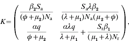
where Sj=Susceptible (j=a for adults and j=r for replacements); βi=transmission parameter (i=1 for adults and i=2 for replacements); q=probability of born infected; α=probability of a parturition resulting in a female calf being born alive; λ=replacement-to-adult transfer rate; φ=per capita BLV-induced death rate; μj=mortality rate (not specific to BLV) (j=1 for replacements and j=2 for adults); N j=total number of animals in a given age group (j=a for adults and j=r for replacements); R 0 is found through computation of the dominant eigenvalue of the next-generation matrix at the disease- or infectious-free equilibrium.
Consequently
with
To explore the relative impact of single factors on R 0 a sensitivity analysis was performed by changing values for single parameters (keeping the rest unchanged) and assessing the percentage of change in R 0. Calculations were performed using Mathematica® (Wolfram Research Inc., USA).
Parameter values
Parameter values for disease transmission were derived from previously published data [Reference Monti, Frankena and De Jong8] (Table 2) and were assumed to be constant over time and equal for the three age groups. Mortality related to BLV infection was only considered for the adult age group because the time needed to develop tumours is longer than the rearing period from calf to adult [Reference Ristau, Beier and Wittmann12].
Table 2. Parameter values used in the simulations
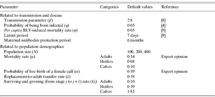
Rates of entry, exit or transition between age groups were calculated based on our previous study, observational data, expert opinions and literature (Table 2). Furthermore, all rates were assumed to be constant over the observation period. Therefore, the probability of growing to the next age group depends on the time spent in the current age group but independent of the time spent in the previous group. The problem is in obtaining information on the probabilities P j (probability of growing) and G j (probability of survival) from information on stage duration. To do this, we separate the processes of survival and growth, both of which appear in P j and G j [Reference Caswell13] by defining:
σj=survival probability (1 – mortality rate for the age group);
T i=residence time (average time that an animal will stay in each age group);
ν=1 (to represent that age distribution within an age group is stable);
λj=probability of growing from j to j+1 given survival) and it was estimated as:

In terms of these parameters [Reference Caswell13]:
P j=σj (1 – λj); probability that an individual in age group j will survive from t to t+1 and staying in stage j;
G j=σjλj; probability of surviving and growing from stage j to j+1.
The entry rate of newborns was calculated as offspring per cow per time unit and it was expressed in terms of female offspring per cow per year. It was estimated based on the standardized (calving interval/365) calving rate per year common in the area, adjusted by the number of stillbirths, calves dead at birth and newborns that die in the first hours after calving (which is estimated as 7%).
For assessing the impact of the different parameters of R 0 we performed a sensitivity analysis by doubling or halving parameters values one by 1.
RESULTS
Default model and parameters settings
First, we evaluated the MSEI model using an average dairy population (n=200) in which initially one infectious individual is introduced in the adult group while the rest of the herd is susceptible. Monte Carlo simulations showed that P minor was ∼10% and the median time to fade-out for minor outbreaks was 64 days with an inter-quartile range of 58 days. The highest prevalence reached for a minor outbreak before going extinct was 3%.
Figure 2 a gives the probability distribution of the prevalence after 1 year, post-introduction and shows a prevalence peak between 0% and 5%. After the second year (Fig. 2 b) the most frequent prevalence was around 30% and after 5 years (Fig. 2 c) between 85% and 95%. At year 30 (Fig. 2 d), the prevalence distribution indicates that a quasi-stationary distribution has been reached as it did not change significantly onwards. Additionally, we extended the simulation for another 50 years, starting from the ‘quasi-stationary distribution’ and no extinction occurred. Because for practical applications the results were clear, simulations were not further extended for a more precise estimation. If the probability of extinction had been 1/100, it should have been found at least once that BLV went extinct with 95% certainty. Because this did not occur the probability of extinction is smaller than 0·001% when starting from the quasi-stationary distribution. Following the same reasoning, the approximation of the expected time to extinction is more than 80 years.
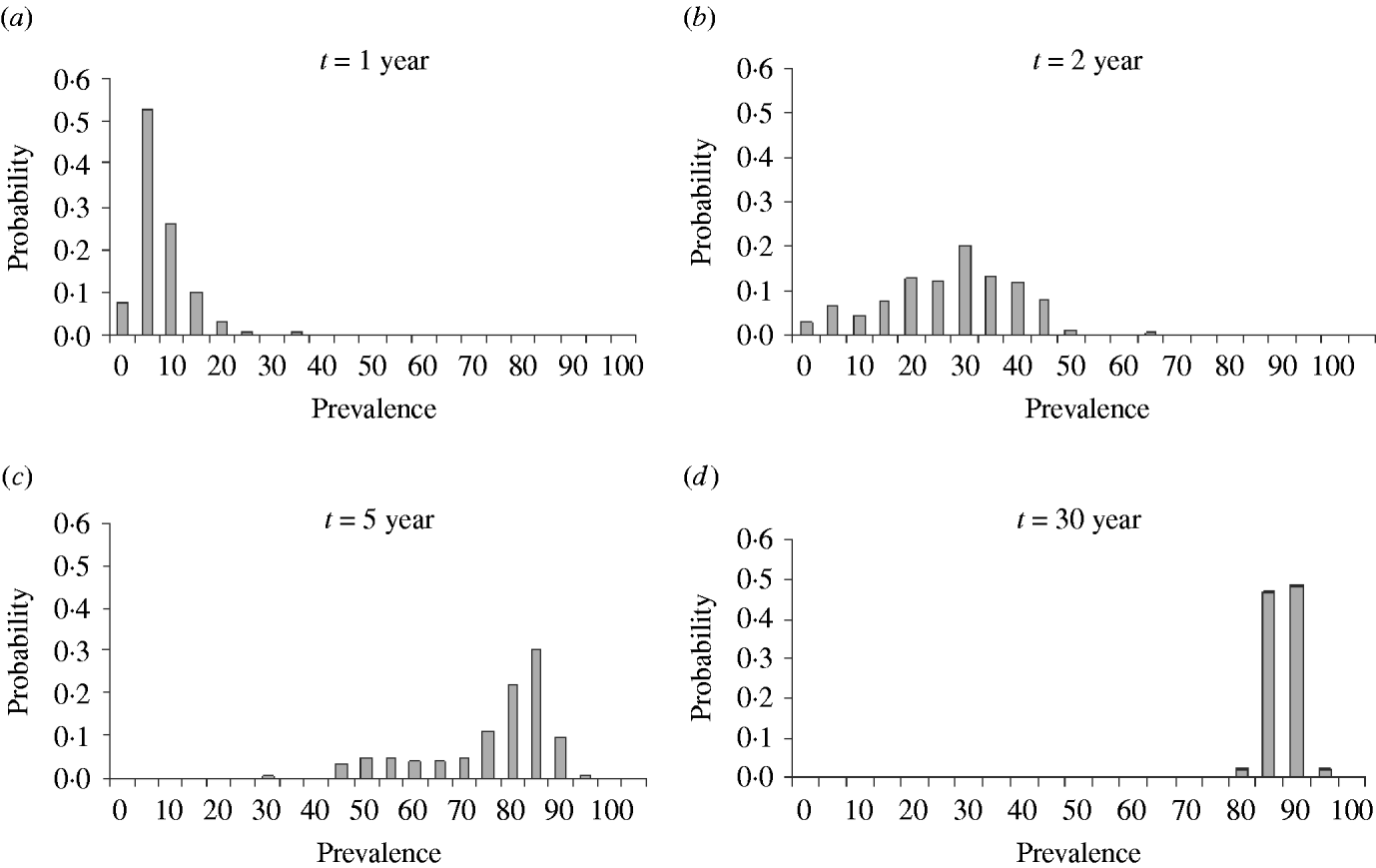
Fig. 2. Probability distribution of prevalence after introduction of an infectious individual in a totally susceptible population of 200 animals after 1, 2, 5 and 30 years.
Effect of model type, herd size and initially infected group on P minor
Table 3 shows the estimations of P minor and the extinction times after introduction of BLV for the various models. When protection by the maternal antibodies state was included in the model, the probability of a minor outbreak was somewhat increased but differences between models were not statistically significant (P>0·05).
Table 3. Probability of minor outbreaks (Pminor) and median time until extinction for four infection models [range and interquartile range (IQR) are also presented]
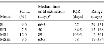
* Kruskal–Wallis χ2 test on extinction times (two-sided)=0·4779, d.f.=3, P value=0·93.
However, when considering the impact of population size on the time to extinction after introduction of BLV, using the MSEI model, the outcomes show that the P minor are quite similar but there are some statistically significant differences between herd sizes 100 and 400 (Table 4).
Table 4. Probability of minor outbreaks (Pminor) and median time till extinction for four herd sizes using a MSEI model [range and interquartile range (IQR) are also presented]
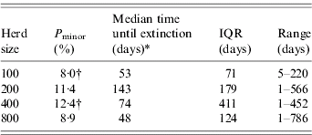
* Kruskal–Wallis χ2 test on extinction times (two-sided)=9·4049, d.f.=3, P value=0·024.
† χ2 test on difference between proportions (reference row is based on size 200).
Finally, P minor and time to extinction were estimated with the introduction of an infectious individual in the group of heifers. Simulation showed a P minor of ∼1% that went extinct in 65 days.
Transmission dynamics of major outbreaks
As for the probability of minor outbreaks, the progress of larger outbreaks also depends on the group where the virus is first introduced. Figure 3 shows results of Monte Carlo simulations after an index case is introduced in age group 3 (adults). At the end of the first year most realizations showed prevalences under 20%. As expected (in the model no cross-infection from adult stock to young stock was assumed) within young stock the prevalence is very low (it started by vertical transmission and then some horizontal transmission may have occurred). After the third year, the prevalence within the adult group increased dramatically (most runs were over 65%). Prevalence, in the replacements group also increased but moderately (<20%). Finally, after 5 years, almost all cows and a great proportion of heifers were infected.
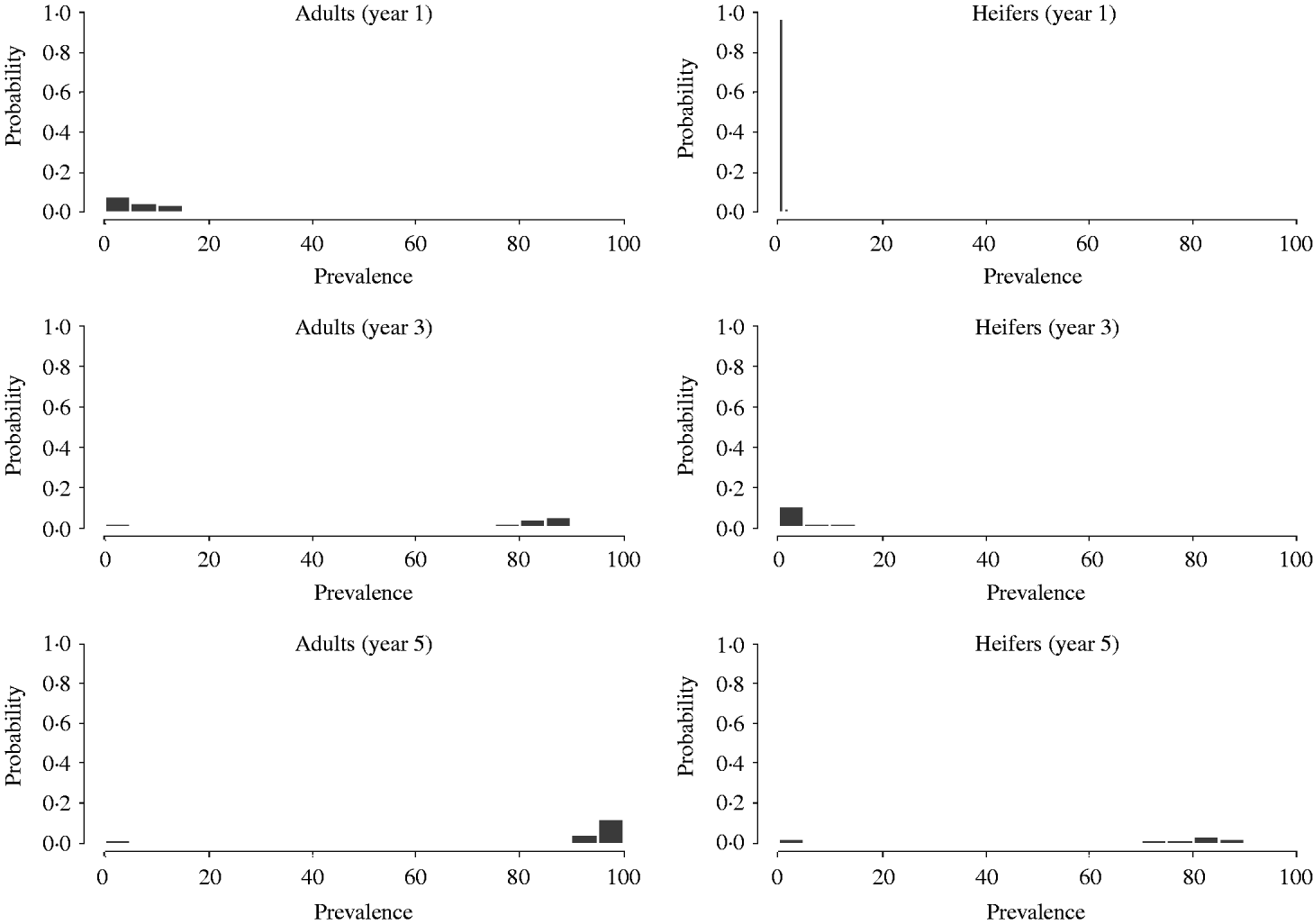
Fig. 3. Distribution of prevalence for age groups 2 and 3, obtained by Monte Carlo simulations, after 1, 3 and 5 years following introduction of a BLV infectious animal in the adult age group.
However, if an index case is introduced in age group 2 (replacements or heifers) (Fig. 4), the prevalence within adults is lower (<15%) and higher in the replacement group at a 1-year time-scale.
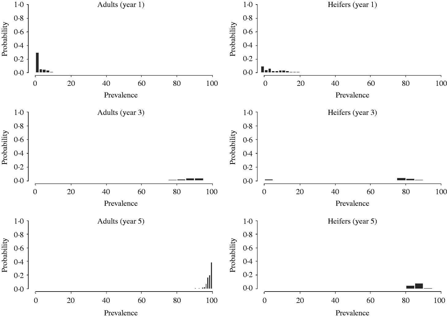
Fig. 4. Distribution of age-group prevalence, obtained by Monte Carlo simulations, after 1, 3 and 5 years following introduction of a BLV infectious animal in the heifers' age group.
After the third year, the prevalence in the adult group increased dramatically and appears quite similar to the distribution in Figure 3. The prevalence within young stock increased dramatically and it is higher than in the previous scenario. Finally, after 5 years, in both age groups almost all cattle appear to be infected. Thus, the overall impact is larger when the virus is introduced in young stock.
Reproduction ratio R 0
The resulting matrix that corresponds to the ‘next-generation operator’ can be represented as:
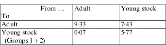
In other words, under the assumptions of this approach, it was estimated that on a per generation basis, one infected adult will infect nine other adults and will produce far less than one infected calf during its infectious reproductive period. In addition, one infected young stock will infect about six other young stock during its rearing period and another 7–8 during its reproductive period. The R 0 was estimated as 9·5.
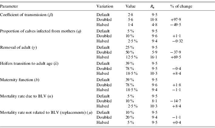
Table 5 summarizes how R 0 changes when we vary parameter settings used for R 0 estimation. From this table we infer that the most influential parameters are: the coefficient of transmission, the removal rate of adults, the mortality rate due to BLV and to a lesser extent the replacement rate from heifers to adults (which reflects the age at first calving of the heifers). For the parameter values used and assumptions stated, elimination is more difficult to achieve by the removal of infected cases.
Table 5. Sensitivity analysis on parameters used to calculate R0
Of the options for within-herd transmission of BLV considered here, some reduction may be achieved by the slaughter of calves born to infected cows (vertical transmission).
Model fit
Figure 5 shows several plots of the model predictions with the observed field data obtained in other studies. Most field observations are within the limits of the 95% CI of the predictions, indicating that simulations mimicked field variations reasonably well.
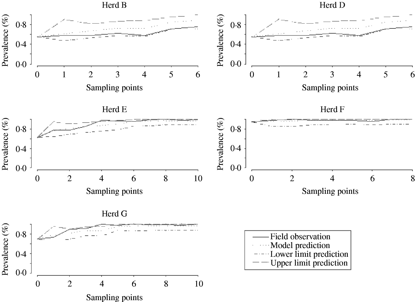
Fig. 5. Validation of model estimations with field data from five herds.
DISCUSSION
In this study we assessed, by Monte Carlo simulation, the transmission model that fits best to the course of a BLV infection in Argentine dairy farms and estimated the probability and time to extinction of BLV. Regarding the latter, the effect of herd size and the age group in which the index case was present were explored further.
Evaluating the fit of the models showed that both the MSEI and the MSI model satisfactorily predict disease transmission as obtained under field conditions. Because inclusion of the latent period did not improve the fit further the MSI model was selected for evaluation of the impact of control measures on transmission. Unfortunately, there are no other modelling studies based on BLV to compare our results with.
Our results indicate that once an infectious individual is present there is a high probability that the disease persists in the herd. However, if it goes extinct, then in most cases it will go extinct relatively quickly. The probability of the disease reaching fade-out after extensive spreading is very low which can be interpreted as not expecting eradication of the disease without any control measure. Moreover, such a high probability of persistence implies that great effort should be placed on prevention of introduction, e.g. by testing all purchased animals and keeping them in quarantine until definite test results are available. In addition, the high persistence of the infection after introduction of BLV is not only important for the single herd but also increases the probability of between-herd transmission when no proper preventive measures are taken. Results indicate that introduction of infection in the heifers group augment – compared to introduction in adult cows – the chances of persistence. Although these concepts have not been evaluated quantitatively before, they have been qualitatively pointed out in previous studies [Reference Gottschau14, Reference Johnson and Kaneene15].
Simulations started with one infectious animal but no particular transmission path that lead to primary infection were considered, therefore, we can not assign the physical introduction to an infected animal. In closed herds, the virus can be introduced by haematophagus insects or by use of blood-contaminated needles or other instruments [Reference Esteban, Sanz and Gogorza16, Reference Rogers17]. Such a risk arises from, for example the way the foot-and-mouth-disease vaccination scheme is implemented or when practitioners do not take proper care of their instruments or via blood-sucking insects [Reference Buxton, Hinkle and Schultz18].
We estimated R 0 as 9·5, and no previous estimations for BLV are available for comparison. Our estimation is similar to R 0 estimations for another retrovirus infection (HIV) which ranges between 9 and 12 [Reference Anderson and May7].
The sensitivity analysis showed that all measures directed to reduce the transmission rate are potentially effective given operational control measures. Previous studies pointed out different ways to decrease transmission, such as reducing the use of mechanical vectors contaminated with blood [Reference DiGiacomo19–Reference Hopkins and DiGiacomo21], insect control [Reference Buxton, Hinkle and Schultz18] or physical contact between infected and susceptible individual [Reference Brunner, Lein and Dubovi22]. In addition, longevity of adult cattle is desirable for production goals, but has a negative impact on BLV persistence as it increases the length of the infectious period. The natural mortality rate also seems to have an important influence on the length of the infectious period.
Our analysis suggests that reduction of vertical transmission will be relatively ineffective since most cases arise through horizontal transmission, as has been suggested before [Reference Hopkins and DiGiacomo21].
CONCLUSIONS
An important prediction of these models is that, even in a relatively small, closed dairy herd, the time-scale for a BLV outbreak may be over 80 years.
One objective of this analysis was to illustrate aspects of BLV epidemiology and control for biologically plausible sets of assumptions and parameter values. The detailed results are obviously sensitive to these assumptions and parameter values. However, the key conclusions appear to be robust: the time-scale of BLV outbreaks within an Argentine dairy herd may be very long and become endemic, and within-herd control of BLV requires intensive efforts.
ACKNOWLEDGEMENTS
The authors thank Dr Aline de Koeijer for her help with R 0 calculations. The research was financed by Secretaria de Ciencia y Técnica de la Nación, PICT no. 08-04541, BID 802 OC-Ar, Argentina.
DECLARATION OF INTEREST
None.


