


Introduction
Fossil assemblages of the soft-bodied Ediacara Biota represent Earth's earliest record of complex multicellular ecosystems. There is general consensus that the Ediacara Biota includes stem-group poriferans, cnidarians, and bilaterians (Erwin and Valentine Reference Erwin and Valentine2013; Erwin Reference Erwin2015, Reference Erwin2021; Cunningham et al. Reference Cunningham, Liu, Bengtson and Donoghue2017; Bobrovskiy et al. Reference Bobrovskiy, Hope, Ivantsov, Nettersheim, Hallman and Brocks2018; Evans et al. Reference Evans, Hughes, Gehling and Droser2020b, Reference Evans, Droser and Erwin2021a; Dunn et al. Reference Dunn, Liu, Grazhdankin, Vixseboxse, Flannery-Sutherland, Green, Harris, Wilby and Donoghue2021, Reference Dunn, Kenchington, Parry, Clark, Kendall and Wilby2022), but most individual taxa remain enigmatic. Despite this, paleobiological and paleoecological studies have revealed information regarding these early organisms, including the nature of their growth (e.g., Dunn et al. Reference Dunn, Liu and Donoghue2018; Evans et al. Reference Evans, Gehling, Erwin and Droser2021b), reproduction (e.g., Droser and Gehling Reference Droser and Gehling2008; Darroch et al. Reference Darroch, Laflamme and Clapham2013; Hall et al. Reference Hall, Droser, Gehling and Dzaugis2015; Mitchell et al. Reference Mitchell, Kenchington, Liu, Matthews and Butterfield2015), and modes of obtaining nutrition (e.g., LaFlamme et al. Reference Laflamme, Xiao and Kowalewski2009; Rahman et al. Reference Rahman, Darroch, Racicot and Laflamme2015; Darroch et al. Reference Darroch, Rahman, Gibson, Racicot and Laflamme2017; Gibson et al. Reference Gibson, Rahman, Maloney, Racicot, Mocke, Laflamme and Darroch2019, Reference Gibson, Darroch, Maloney and Laflamme2021). The common in situ preservation of fossils of the Ediacara Biota has also allowed for examination of the spatial distributions of fossil communities, providing a dataset, unusual for the fossil record, that can be used to test hypotheses about life histories (Clapham et al. Reference Clapham, Narbonne and Gehling2003; Hall et al. Reference Hall, Droser, Gehling and Dzaugis2015; Mitchell et al. Reference Mitchell, Kenchington, Liu, Matthews and Butterfield2015, Reference Mitchell, Kenchington, Harris and Wilby2018, Reference Mitchell, Bobkov, Bykova, Dhungana, Kolesnikov, Hogarth, Liu, Mustill, Sozonov, Rogov, Xiao and Grazhdankin2020, Reference Mitchell, Evans, Chen and Xiao2022; Coutts et al. Reference Coutts, Bradshaw, García-Bellido and Gehling2018; Gehling and Droser Reference Gehling and Droser2018; Mitchell and Butterfield Reference Mitchell and Butterfield2018; Mitchell and Kenchington Reference Mitchell and Kenchington2018; Vixseboxse et al. Reference Vixseboxse, Kenchington, Dunn and Mitchell2021).
In the Flinders Ranges area of South Australia, the Ediacara Member of the Rawnsley Quartzite consists of shallow-marine deposits characterized by well-preserved in situ fossils of the White Sea Assemblage (Gehling Reference Gehling2000). A new unit, the Nilpena Member, characterized by a basal incision, has been informally described and consists of the upper tens of meters of what was previously included in the Ediacara Member (Gehling et al. Reference Gehling, García-Bellido, Droser, Tarhan and Runnegar2019). Within these two units, taxa of the Ediacara Biota are preserved as casts and molds on the bases of sandstone beds (Gehling Reference Gehling1999). At Nilpena Ediacara National Park (NENP), the excavation and reconstruction of 40 discrete beds, 33 of which preserve at least 10 body fossils, provides approximately 350 m2 of Ediacaran seafloor (Fig. 1A). Such an extensive area permits the detailed reconstruction of “snapshots” of Ediacaran communities and provides the opportunity to examine the spatial distributions of constituent populations.
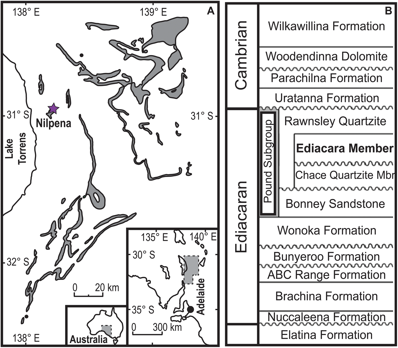
Figure 1. A, Distribution of the Pound Subgroup outcrops (gray) bearing the most prominent Ediacaran fossils horizons. Nilpena Ediacara National Park (NENP) is marked by a purple star. B, Stratigraphic locations of the Ediacara Member. Modified from Gehling and Droser (Reference Gehling and Droser2009).
Although seven Ediacaran taxa have been cited as potentially mobile (Evans et al. Reference Evans, Gehling and Droser2019), the majority of taxa from the Ediacara Member were sessile and lived atop or embedded in laterally extensive microbial mats (Droser et al. Reference Droser, Gehling, Tarhan, Evans, Hall, Hughes, Hughes, Dzaugis, Dzaugis, Dzaugis and Rice2019, Reference Droser, Evans, Tarhan, Surprenant, Hughes, Hughes and Gehling2022). These mats were abundant in the absence of widespread bioturbation and range in maturity between beds at NENP (Droser et al. Reference Droser, Evans, Tarhan, Surprenant, Hughes, Hughes and Gehling2022). Among the sessile organisms, the triradialomorph taxa Tribrachidium and Rugoconites occur in both South Australia and the White Sea of Russia and are abundant at NENP (Glaessner and Daily Reference M. F. and Daily1959; Glaessner and Wade Reference Glaessner and Wade1966; Hall et al. Reference Hall, Droser, Gehling and Dzaugis2015, Reference Hall, Droser and Gehling2018; Boag et al. Reference Boag, Darroch and Laflamme2016). Other sessile taxa, such as the newly described and asymmetrical Obamus coronatus, as yet occur only at NENP (Dzaugis et al. Reference Dzaugis, Evans, Droser, Gehling and Hughes2018).
These three enigmatic taxa have similar diameters and general shapes, but exhibit different bed-to-bed distributions at NENP (Hall et al. Reference Hall, Droser, Gehling and Dzaugis2015, Reference Hall, Droser and Gehling2018; Dzaugis et al. Reference Dzaugis, Evans, Droser, Gehling and Hughes2018; Droser et al. Reference Droser, Gehling, Tarhan, Evans, Hall, Hughes, Hughes, Dzaugis, Dzaugis, Dzaugis and Rice2019). Here we examine the spatial distribution of Tribrachidium, Rugoconites, and Obamus on five excavated beds at NENP through the application of spatial point pattern analysis (SPPA) to determine their spatial distributions and to test hypotheses regarding their life histories, including settlement and dispersal, and potential interactions with their environments. In modern marine invertebrate populations, dispersal mechanisms affect the small- and large-scale spatial distributions of organisms (Wangensteen et al. Reference Wangensteen, Turon, Placin, Rossi, Bramanti, Gori and Orejas2016). Availability of substrate also plays a role during dispersal and settlement, along with preexisting conspecific distributions (e.g., Rodríguez et al. Reference Rodríguez, Ojeda and Inestrosa1993; Sampayo et al. Reference Sampayo, Roff, Sims, Rachello-Dolmen and Pandolfi2020). SPPA takes into consideration common pitfalls in the field of spatial ecology (irregularly shaped study areas, edge effect, etc.) and thus, is ideally suited for Ediacaran surfaces (Wiegand et al. Reference Wiegand, Kissling, Cipriotti and Aguiar2006). This study examines small-scale (individual-bed surface distributions) and large-scale data (bed-to-bed distributions) of Tribrachidium, Rugoconites, and Obamus to determine the possible role of dispersal mechanisms and/or environmental factors controlling their distributions.
Geologic Setting and Material
The Flinders Ranges region of South Australia contains one of the best exposed and most complete successions of Neoproterozoic-aged rocks in the world, including the type section of the Ediacaran Period. Within this succession, the siliciclastic, sandstone-dominated Ediacara Member and new informal Nilpena Member of the Rawnsley Quartzite contain an extensive record of the Ediacara Biota, cropping out with varying thickness between 10 to 300 m (Gehling Reference Gehling2000; Tarhan et al. Reference Tarhan, Droser and Gehling2015a; Droser et al. Reference Droser, Gehling, Tarhan, Evans, Hall, Hughes, Hughes, Dzaugis, Dzaugis, Dzaugis and Rice2019; Gehling et al. Reference Gehling, García-Bellido, Droser, Tarhan and Runnegar2019; Fig. 1B). At NENP, west of the Flinders Ranges, a combination of preservation and exposure of the Ediacara and Nilpena Members has uniquely facilitated the excavation and reconstruction of discrete and fossiliferous bedding planes. Their excavation has enabled detailed reconstruction of the ecology, habitat, and fossilization of Ediacaran communities (e.g., Droser et al. Reference Droser, Tarhan, Evans, Surprenant and Gehling2020; Evans et al. Reference Evans, Dzaugis, Droser and Gehling2020a; Surprenant et al. Reference Surprenant, Gehling and Droser2020; Tarhan et al. Reference Tarhan, Droser and Gehling2022). Importantly, the shapes and sizes of these beds are a function of geology (e.g., faults), logistics (the beds dip too deeply under the surface), and taphonomy (the bedding surface loses preservational integrity; Hall et al. Reference Hall, Droser, Gehling and Dzaugis2015; Droser et al. Reference Droser, Gehling, Tarhan, Evans, Hall, Hughes, Hughes, Dzaugis, Dzaugis, Dzaugis and Rice2019). The 33 beds with more than 10 body fossils range in size from 1 to 23 m2 and represent, in total, more than 350 m2 of Ediacaran seafloor. Numerous beds are excavated from a single pit and represent continuous stratigraphic successions interbedded with submillimeter- to millimeter-scale beds known as “shims” (Droser et al. Reference Droser, Gehling, Tarhan, Evans, Hall, Hughes, Hughes, Dzaugis, Dzaugis, Dzaugis and Rice2019).
At NENP, fossiliferous surfaces have been excavated from the Oscillation-Rippled Sandstone Facies (ORS) and the Planar-Laminated and Rip-Up Sandstone Facies (PLRUS; Gehling and Droser Reference Gehling and Droser2013; Droser et al. Reference Droser, Tarhan and Gehling2017, Reference Droser, Gehling, Tarhan, Evans, Hall, Hughes, Hughes, Dzaugis, Dzaugis, Dzaugis and Rice2019; Tarhan et al. Reference Tarhan, Droser, Gehling and Dzaugis2017). The ORS Facies is characterized by submillimeter- to centimeter-thick, rippled, fine- to coarse-grained quartz sandstones interpreted to have been deposited under oscillatory and combined flow between fair-weather- and storm-wave base (Tarhan et al. Reference Tarhan, Droser, Gehling and Dzaugis2017; Droser et al. Reference Droser, Gehling, Tarhan, Evans, Hall, Hughes, Hughes, Dzaugis, Dzaugis, Dzaugis and Rice2019). The PLRUS Facies consists of laterally continuous, planar-laminated, fine-grained sandstone beds and is interpreted to have been deposited under unidirectional flow in a sub–wave base upper canyon fill (Gehling and Droser Reference Gehling and Droser2013; Droser et al. Reference Droser, Gehling, Tarhan, Evans, Hall, Hughes, Hughes, Dzaugis, Dzaugis, Dzaugis and Rice2019). Fossils in both facies occur primarily as external molds on the base of beds. Five beds were used for this study. Bed SE-Rugo, from the ORS Facies, is the only excavated surface within the Ediacara Member with more than 20 specimens of Rugoconites. The majority of beds with Rugoconites have dispersed populations of fewer than 10 individuals (Table 1). LV-FUN is abundantly populated by Obamus and is from the PLRUS Facies. Tribrachidium dominates two beds and occurs in an abundance greater than 20 on a third: beds 1T-T and TC-MM3 are from the ORS Facies, while bed WS-TBEW is from the PLRUS Facies. The WS-TBEW bed consists of two non-joining parts, and these are considered separate surfaces for the sake of this study: WS-TBE and WS-TBW.
Table 1. Adapted from Droser et al. Reference Droser, Gehling, Tarhan, Evans, Hall, Hughes, Hughes, Dzaugis, Dzaugis, Dzaugis and Rice2019. Beds at Nilpena Ediacara National Park (NENP) on which Tribrachidium, Rugoconites, and Obamus occur. Note that while WS-TBE and WS-TBW are from the same bedding surface, they have been separated here for statistical interpretations. Bold rows indicate beds being examined here.

Tribrachidium is a triradially symmetrical taxon occurring in both the ORS and PLRUS Facies at NENP and the White Sea region of Russia (Glaessner and Daily Reference M. F. and Daily1959; Grazhdankin and Ivantsov Reference Grazhdankin and Yu. Ivantsov1995; Martin et al. Reference Martin, Grazhdankin, Bowring, Evans, Fedonkin and Kirschvink2000; Boag et al. Reference Boag, Darroch and Laflamme2016; Ivantsov and Zakrevskaya Reference Ivantsov and Zakrevskaya2021; Fig. 2A). Tribrachidium ranges in size from 0.2 to 4 cm in diameter and occurs in negative hyporelief on the base of 12 surfaces at NENP, with populations ranging from single individuals on a surface to more than 100 (Hall et al. Reference Hall, Droser, Gehling and Dzaugis2015; Rahman et al. Reference Rahman, Darroch, Racicot and Laflamme2015; Droser et al. Reference Droser, Gehling, Tarhan, Evans, Hall, Hughes, Hughes, Dzaugis, Dzaugis, Dzaugis and Rice2019; Table 1). Both normal and log-normal size–frequency distributions of Tribrachidium from NENP suggest that they lived in single-generation populations and reproduced seasonally (Hall et al. Reference Hall, Droser, Gehling and Dzaugis2015). Additionally, Tribrachidium has been interpreted as a passive suspension feeder, based on computational fluid dynamics (Rahman et al. Reference Rahman, Darroch, Racicot and Laflamme2015). Tribrachidium is associated with the fossil form “concentric circles” (Hall et al. Reference Hall, Droser, Gehling and Dzaugis2015; also called concentric ridges or grooves; Glaessner and Wade Reference Glaessner and Wade1966; Fedonkin Reference Fedonkin, Ivanovsky and Ivanov1984). These are interpreted to represent specimens that were flipped before or during episodic burial (preserved as external molds in negative hyporelief) or the cavity left by an organism entirely removed from the seafloor (preserved in positive hyporelief; Fedonkin Reference Fedonkin, Ivanovsky and Ivanov1984; Hall et al. Reference Hall, Droser, Gehling and Dzaugis2015). Thus, concentric circles preserved in positive hyporelief are viable for spatial statistical analysis, because they record the presence of a Tribrachidium, while negative relief external molds are not viable for spatial statistics, because they record a transported specimen. Previous nearest-neighbor analyses suggested that one population of Tribrachidium at NENP was distributed randomly (Bed 1T-T; Hall et al. Reference Hall, Droser, Gehling and Dzaugis2015).

Figure 2. A, Tribrachidium, a triradial taxon found at Nilpena Ediacara National Park (NENP) and the White Sea of Russia. B, Rugoconites, another triradial taxon found in Australia and the White Sea. C, Obamus, a torus-shaped taxon found only at NENP. As it was deeply embedded in the microbial mat a Silly Putty mold (right) was placed next to the individual to show what the organism would have looked like on the seafloor. Scale bars, 1 cm.
Rugoconites is another triradial taxon that occurs in Australia and Russia, with a single poorly preserved possible specimen reported from Canada (Glaessner and Wade Reference Glaessner and Wade1966; Narbonne and Hofmann Reference Narbonne and Hofmann1987; Hall et al. Reference Hall, Droser, Gehling and Dzaugis2015, Reference Hall, Droser and Gehling2018; Fig 2B). Rugoconites is generally circular and has a size range of 1 to 6 cm in diameter (Glaessner and Wade Reference Glaessner and Wade1966; Hall et al. Reference Hall, Droser, Gehling and Dzaugis2015, Reference Hall, Droser and Gehling2018). Specimens occur in negative hyporelief on the base of 14 surfaces at NENP in both the PLRUS and ORS Facies, with the majority of populations consisting of fewer than 10 individuals (Table 1). The size–frequency distributions of Rugoconites suggest that, similar to Tribrachidium, populations were composed of single generations or cohorts (Hall et al. Reference Hall, Droser and Gehling2018). As with Tribrachidium, analyses were run on both normal and log-normal body-size diameters, with the same results for each (Hall et al. Reference Hall, Droser and Gehling2018). Both Tribrachidium and Rugoconites have been interpreted to be environmental generalists, based on their wide environmental distributions and association with both mature and immature microbial mats and a variety of other taxa (Grazhdankin and Ivanstov Reference Grazhdankin and Yu. Ivantsov1995; Hall et al. Reference Hall, Droser, Gehling and Dzaugis2015, Reference Hall, Droser and Gehling2018; Droser et al. Reference Droser, Gehling, Tarhan, Evans, Hall, Hughes, Hughes, Dzaugis, Dzaugis, Dzaugis and Rice2019).
Obamus is a torus-shaped organism that lived embedded in the microbial mat that covered the Ediacaran seafloor. It is preserved in negative hyporelief (Dzaugis et al. Reference Dzaugis, Evans, Droser, Gehling and Hughes2018; Fig 2C). Specimens of Obamus have been identified on four surfaces from both the ORS and PLRUS Facies (Table 1). Previous studies have noted that Obamus appears to be common in areas of mature organic mats (Dzaugis et al. Reference Dzaugis, Evans, Droser, Gehling and Hughes2018; Droser et al. Reference Droser, Evans, Tarhan, Surprenant, Hughes, Hughes and Gehling2022). Unlike Tribrachidium and Rugoconites, which both occur on multiple continents with significant paleogeographic separation (Grazhdankin and Ivanstov Reference Grazhdankin and Yu. Ivantsov1995; Hall et al. Reference Hall, Droser, Gehling and Dzaugis2015, Reference Hall, Droser and Gehling2018; Droser et al. Reference Droser, Gehling, Tarhan, Evans, Hall, Hughes, Hughes, Dzaugis, Dzaugis, Dzaugis and Rice2019), Obamus has thus far only been found at NENP and only in association with mature microbial mats.
Spatial Distributions
The spatial distribution of sessile organisms can be used to test hypotheses about reproductive strategies, competition, and environmental impacts (Kenkel Reference Kenkel1988; Harms et al. Reference Harms, Wright, Calderon, Hernandez and Herre2000; He and Legendre Reference He and Legendre2002; Atkinson et al. Reference Atkinson, Foody, Gething, Mathur and Kelly2007; Jacquemyn et al. Reference Jacquemyn, Brys, Vandepitte, Honnay, Roldan-Ruiz and Wiegand2007; Watson et al. Reference Watson, Roshier and Wiegand2007; Wiegand et al. Reference Wiegand, Gunatilleke and Gunatilleke2007a; Law et al. Reference Law, Illian, Burslem, Gratzer, Gunatilleke and Gunatilleke2009; Franklin and Santos Reference Franklin and Santos2010; Zillio and He Reference Zillio and He2010; Lin et al. Reference Lin, Chang, Yang, Wang and Sun2011; Schleicher et al. Reference Schleicher, Meyer, Wiegand, Schurr and Ward2011; Chang and Marshall Reference Chang and Marshall2016; Carrer et al. Reference Carrer, Castagneri, Popa, Pividori and Lingua2018; Mitchell and Harris Reference Mitchell and Harris2020). Distributions can be described as either aggregated, random, or segregated (Fig. 3). In both terrestrial and marine ecosystems, aggregation (also described as clustering or clumping) is by far the most common distribution, often resulting from dispersal limitations and/or environmental controls (Carlon and Olson Reference Carlon and Oslon1993; Karlson et al. Reference Karlson, Hughes and Karlson1996; He and Legendre Reference He and Legendre2002; Franklin and Santos Reference Franklin and Santos2010; Lin et al. Reference Lin, Chang, Yang, Wang and Sun2011; Carrer et al. Reference Carrer, Castagneri, Popa, Pividori and Lingua2018; Lesneski et al. Reference Lesneski, D'Aloia, Fortin and Buston2019; Ben-Said Reference Ben-Said2021; Fig. 3A). Mathematically, an aggregated pattern is one in which the neighborhood density (the number of points separated by a distance) is high enough that points tend to be located nearer to each other than expected based on a random null model (Wiegand and Moloney Reference Wiegand and Moloney2014). For example, strongly aggregated patterns of sexually reproducing marine benthic invertebrates can be the result of habitat-selective larval stages, short-lived/dispersed larval stages, and/or a preference for being near conspecifics (Carlon and Olson Reference Carlon and Oslon1993).

Figure 3. Common types of spatial distributions found in modern ecosystems. Small purple dots indicate the locations of individuals of a certain taxon. A, Aggregation: individuals being closer together than would be predicted in a random distribution. B, Randomness: individuals are in a Poisson distribution. C, Segregation: points are farther apart than predicted in a random distribution, resulting in a uniform pattern. D, Thomas cluster (medium orange circles): individuals are aggregated around a center point at varying distances. E, Double Thomas cluster (large blue circles): a nested cluster pattern in which two sets of clusters are present at two spatial scales.
Random patterns are less common in modern ecosystems but have been associated with certain marine organisms as a function of settlement (Schmidt Reference Schmidt1982; Guy-Haim et al. Reference Guy-Haim, Rilov and Achituv2015; Fig. 3B). For example, the southern Californian bryozoan Bugula neritina has random distributions due to larvae not having a preference for substrate or being near a conspecific (Keough Reference Keough1984). At the ecosystem scale, a random pattern has been interpreted to represent a community whose distribution is not controlled by biological (dispersal limitations, settlement preference, etc.) or environmental constraints (limited resource, widely dispersed patches, etc.; Davis and Campbell Reference Davis and Campbell1996; Brenchley and Harper Reference Brenchley and Harper1998). Mathematically, random distributions are Poisson processes wherein points are randomly and independently located within an area (Wiegand and Moloney Reference Wiegand and Moloney2014; Velázquez et al. Reference Velázquez, Martínez, Getzin, Moloney and Wiegand2016; Ben-Said Reference Ben-Said2021).
Organisms can also be segregated (also known as regular, uniform, or hyperdispersed) and, like aggregation, segregation is determined through comparison with the null model of a random distribution (Ben-Said Reference Ben-Said2021). Mathematically, this pattern occurs when the neighborhood density is lower than a random pattern, resulting in points that are regularly spread out (Wiegand and Moloney Reference Wiegand and Moloney2014; Fig 3C). Ecologically, this distribution is associated with competition, specifically intraspecific competition, as individuals will maintain a certain distance apart to ensure resource acquisition occurs without competition, or habitat association, where the underlying habitat is segregated (Kenkel Reference Kenkel1988; Brenchley and Harper Reference Brenchley and Harper1998; Lin et al. Reference Lin, Chang, Yang, Wang and Sun2011; Mitchell and Kenchington Reference Mitchell and Kenchington2018). Additionally, segregation can be a result of habitat patchiness (Mitchell and Kenchington Reference Mitchell and Kenchington2018). For example, the modern South Australian ascidian Clavelina moluccensis has been noted to settle in a segregated (regular) pattern as a result of interspecific competition (Davis and Campbell Reference Davis and Campbell1996).
The bed-scale spatial distributions of Rugoconites and Obamus have not previously been examined, and only one population of Tribrachidium at NENP has been analyzed for spatial distribution (1T-T = random distribution via nearest-neighbor analysis; Hall et al. Reference Hall, Droser, Gehling and Dzaugis2015). Using SPPA instead of nearest-neighbor analysis allows greater spatial scales to be covered. Here we examine the spatial patterns of these benthic sessile taxa on six different surfaces in order test possible biological and ecological controls on their distributions and gain insight into their reproductive and dispersal methods.
Methods
Spatial distributions of Tribrachidium, Rugoconites, and Obamus were analyzed from six surfaces at NENP. Surfaces were logged and mapped using a centimeter-scale grid (Fig. 4, Supplementary Fig. 1) (for more information on bed mapping, see Droser et al. [2019]). To control for possible variations in preservation potential across each surface, each bed was examined on the centimeter scale for variations in preservation of textured organic surfaces (mats). If there were preservational gaps in the mat and/or the surface was fretted, we digitally removed that area. Specifically, we only included areas of the bed in which both the mat texture and the organism are clearly preserved and in situ. Using this approach, fretted portions of both TC-MM3 (original area = 21.56 m2; edited area = 17 m2) and 1T-T (original area = 4.4 m2; edited area = 4.1 m2) were digitally excluded.

Figure 4. Excavated surfaces examined in this paper. This figure only shows Tribrachidium, Rugoconites, and Obamus locations on their respective beds. Other taxa were left out for the convenience of the reader. Dots are not to scale. Note that surfaces WS-TBE and WS-TBW are from the same bed, but were unable to be attached during excavation. As such, they are treated as two separate surfaces here. Additionally, locations on TC-MM3 with poor preservation were removed to account for taphonomic heterogeneity. A–D, Tribrachidium populations are plotted in different shades of pink. E, Rugoconites populations are plotted in orange. F, Obamus populations are plotted in blue.
To capture both the irregular shapes and edges of the surfaces, hundreds of photographs were taken and compiled in the photogrammetric 3D modeling software Agisoft Metashape (field methods adapted from Mallison and Wings [Reference Mallison and Wings2014]). The borders of the surfaces were then drawn out in ArcGIS to create borders accurate to the millimeter-scale in which the taxa coordinates are plotted. Because the shapes, sizes, and population densities of taxa are out of excavators’ control, excavated surfaces at NENP act as “random” samples of Ediacaran ecosystems.
The six surfaces were chosen based on the number of individual Tribrachidium, Rugoconites, or Obamus present on each surface, with a minimum requirement of 20 individuals per surface (Table 1). Concentric circles preserved in positive relief on WS-TBE and WS-TBW were included in combination with classically preserved Tribrachidium, as they represent the locations of specimens “pulled out” before burial, presumably by a storm (Hall et al. Reference Hall, Droser, Gehling and Dzaugis2015). Negative hyporelief concentric circles on 1T-T were not used, because they are interpreted as non–in situ Tribrachidium that have been pulled out; however, the few positive concentric circles on that surface were used (Hall et al. Reference Hall, Droser, Gehling and Dzaugis2015).
Bed-to-bed distributions of taxa were determined using data published by Droser et al. (Reference Droser, Gehling, Tarhan, Evans, Hall, Hughes, Hughes, Dzaugis, Dzaugis, Dzaugis and Rice2019) on density (number of individuals/square meters) and abundance within each of the two facies and excavation sites (Table 1). Bed surface-scale spatial distributions of each taxon were tested against a random pattern to identify aggregation, segregation, or a lack thereof via SPPA in Programita and the R package Spatstat (Wiegand and Moloney Reference Wiegand and Moloney2014; Baddeley et al. Reference Baddeley, Rubak and Turner2016). Previous studies have used SPPA to investigate the distributions of the Ediacara Biota (Mitchell et al. Reference Mitchell, Kenchington, Liu, Matthews and Butterfield2015, Reference Mitchell, Kenchington, Harris and Wilby2018, Reference Mitchell, Bobkov, Bykova, Dhungana, Kolesnikov, Hogarth, Liu, Mustill, Sozonov, Rogov, Xiao and Grazhdankin2020; Coutts et al. Reference Coutts, Bradshaw, García-Bellido and Gehling2018; Mitchell and Butterfield Reference Mitchell and Butterfield2018; Mitchell and Kenchington Reference Mitchell and Kenchington2018). The work presented here is the first use of SPPA to interpret Tribrachidium, Rugoconites, and Obamus distributions.
SPPA is divided into three major statistical components that allow for biological and ecological characteristics to be interpreted.
Summary Statistics
Summary statistics quantify the properties of an observed pattern using functions of distance. Multiple summary statistics are required for a complete analysis (Franklin and Santos Reference Franklin and Santos2010; Wiegand and Moloney Reference Wiegand and Moloney2014). Summary statistics can be divided into two categories: first-order summary statistics, or those which examine the configuration of individual points; and second-order summary statistics, which are based on the spatial relationships of pairs of points (Wiegand and Moloney Reference Wiegand and Moloney2014). The main summary statistic used here is the pair-correlation function (PCF), which is a second-order summary statistic that calculates the pairwise distance from each point to each other point, and then establishes how many points are found within a given radius (r) from the average/typical point (Illian et al. Reference Illian, Penttinen, Stoyan and Stoyan2008; Wiegand and Moloney Reference Wiegand and Moloney2014; Velázquez et al. Reference Velázquez, Martínez, Getzin, Moloney and Wiegand2016). PCF will continue to examine pairs at different distances until the range of correlation (r corr) is reached. The range of correlation is the distance at which PCF is no longer statistically relevant due to the shape and size of the study area, and typically is half the width of the thinnest part of the study area (Illian et al. Reference Illian, Penttinen, Stoyan and Stoyan2008; Baddeley et al. Reference Baddeley, Rubak and Turner2016). The L-function (LF) was also used to examine the distributions on selected surfaces. This method examines the number of points within a circle whose radius is r, and will continue to increase in size till the r corr is reached. The LF was used to support PCF results, and LF plots are provided in Supplementary Figures 2–4.
Null Models
Both the LF and PCF were used in tandem with null models—patterns that represent a null hypothesis or standards to which an observed population's distribution is compared (Wiegand and Moloney Reference Wiegand and Moloney2014; Velázquez et al. Reference Velázquez, Martínez, Getzin, Moloney and Wiegand2016). Null models are based on the number of points within a study area and their reorientation into common spatial patterns (e.g., a random pattern; Wiegand and Moloney Reference Wiegand and Moloney2014; Velázquez et al. Reference Velázquez, Martínez, Getzin, Moloney and Wiegand2016). For the work presented here, each null model was run through 999 Monte Carlo simulations. The highest and lowest 49 Monte Carlo simulation values were taken to create a simulation envelope (see “Confidence Tests”). We chose 999 Monte Carlo simulations because the higher number of simulations used will increase the accuracy of the simulation envelope (Velázquez et al. Reference Velázquez, Martínez, Getzin, Moloney and Wiegand2016) and 999 is considered large without being too computationally taxing (Wiegand and Moloney Reference Wiegand and Moloney2014). The highest and lowest 49 values were chosen, as they are the upper and lower 5% of the simulated data and result in a probability error of 0.05 as recommended by Illian et al. (Reference Illian, Penttinen, Stoyan and Stoyan2008). The summary statistic line was then plotted over the simulation envelope, revealing the spatial scales at which a positive (above the simulation envelope), negative (below the simulation envelope), or neutral (within the simulation envelope) relationship is present.
In these plots the x-axis represents the radius from the center of each specimen and the y-axis is the summary statistical function value. The higher the function value, the stronger the spatial pattern, and vice versa (Dhungana and Mitchell Reference Dhungana and Mitchell2021). The first (and primary) null model tested was complete spatial randomness (CSR), also known as the homogenous Poisson null model, which determines if a pattern is random, aggregated, or segregated. While the CSR null model is suitable for determining the gross spatial distribution of organisms, it is best used in tandem with other models, such as the heterogenous Poisson (HP) null model, to determine the most likely underlying process behind nonrandom patterns (Wiegand and Moloney Reference Wiegand and Moloney2014). The HP null model determines whether a pattern is random (i.e., points are independently distributed) while allowing the intensity (density) of points in an area to vary depending on location (Wiegand et al. Reference Wiegand, Gunatilleke and Gunatilleke2007a; Schleicher et al. Reference Schleicher, Meyer, Wiegand, Schurr and Ward2011; Wiegand and Moloney Reference Wiegand and Moloney2014; Velázquez et al. Reference Velázquez, Martínez, Getzin, Moloney and Wiegand2016; Carrer et al. Reference Carrer, Castagneri, Popa, Pividori and Lingua2018). As this method accounts for varying densities, the HP null model has been used to identify environmental heterogeneities in an ecosystem (soil nutrients, topography, etc.; Wiegand et al. Reference Wiegand, Gunatilleke and Gunatilleke2007a; Wiegand and Moloney Reference Wiegand and Moloney2014; Velázquez et al. Reference Velázquez, Martínez, Getzin, Moloney and Wiegand2016; Carrer et al. Reference Carrer, Castagneri, Popa, Pividori and Lingua2018). Thus, the HP model assesses whether the observed patterns are the same, more aggregated, or more segregated than the null model, whereas the CSR model is the only model that determines absolute randomness, aggregation, and segregation.
If a population was determined to be aggregated, we also tested for a Thomas cluster (TC) and double Thomas cluster (DTC), aggregation patterns common in modern taxa (Wiegand et al. Reference Wiegand, Gunatilleke, Gunatilleke and Okuda2007b). The TC null model determines whether individuals are aggregated around a center point at varying distances with randomly distributed cluster centers (Wiegand et al. Reference Wiegand, Martínez and Huth2009; Wiegand and Moloney Reference Wiegand and Moloney2014; Fig. 3D). The TC can be further analyzed to determine whether the pattern fits a nested cluster, more commonly known as DTC (Fig. 3E). In this model, smaller TCs are located within the larger DTC, and cluster centers are not random (Wiegand et al. Reference Wiegand, Martínez and Huth2009). Determining whether organism distributions fit a TC and DTC has been used to investigate the dispersal of offspring in a given area for both modern and fossilized ecosystems (Wiegand et al. Reference Wiegand, Martínez and Huth2009; Mitchell et al. Reference Mitchell, Kenchington, Liu, Matthews and Butterfield2015; Mitchell and Harris Reference Mitchell and Harris2020; Dhungana and Mitchell Reference Dhungana and Mitchell2021). While the TC and DTC null models are sometimes referred to as the CSR+TC and CSR+DTC null models, we choose to refer to them as the former, which are more consistent with current literature (e.g., Mitchell et al. Reference Mitchell, Bobkov, Bykova, Dhungana, Kolesnikov, Hogarth, Liu, Mustill, Sozonov, Rogov, Xiao and Grazhdankin2020; Dhungana and Mitchell Reference Dhungana and Mitchell2021).
Finally, to rule out environmental heterogeneity as a driver of distribution patterns among Tribrachidium, Rugoconites, and Obamus, populations were tested against a heterogenous Poisson Thomas cluster (HPTC) and heterogenous Poisson double Thomas cluster (HPDTC). These methods were used to determine whether any form of heterogeneity, and specifically environmental heterogeneity, was present. Similar to the manner in which TC and DTC determine whether a surface has individuals aggregated around a center point (TC) or whether those clusters are nested (DTC), the HPTC and HPDTC methods determine whether the population fits those patterns while also considering how the intensity of the pattern varies depending on the locations of the points within the study area. It is important to note that nested clusters can also occur when you have TC on a background HP aggregation, so it is prudent to test for DTC versus HPTC to determine whether there are multiple reproductive events or a single reproductive event with environmental filtering.
Confidence Tests
To determine whether certain patterns fit a specific null model, the analytical global envelope (AGE) was used, and are depicted as the colored simulation envelopes in our results (shades of pink = Tribrachidium, orange = Rugoconites, blue = Obamus). The AGE was chosen because it incorporates information on the number of individuals, the size and shape of the fossil surfaces, other aspects of the summary statistics lost during a pointwise simulation envelope (indicated as the black dotted line within the colored simulation envelope) and is the more popular method (Wiegand et al. Reference Wiegand, Grabarnik, P. and Stoyan2016). It is important to note that the more points (in this case, fossils) included in a test, the thinner the AGE will be.
We also used goodness-of-fit (GoF; referred to as “pd” in text) tests to determine whether taxon patterns matched any of the null models. The GoF is similar to a p-value: a value of 0.0 indicating a complete rejection of the specific null model, while 1.0 indicates a perfect fit (Mitchell et al. Reference Mitchell, Bobkov, Bykova, Dhungana, Kolesnikov, Hogarth, Liu, Mustill, Sozonov, Rogov, Xiao and Grazhdankin2020). It is vital to note that GoF tests are only used in an auxiliary fashion and cannot override a visual inspection of the AGE and summary statistic plot (Wiegand and Moloney Reference Wiegand and Moloney2014).
Three rounds of smoothing were done on each surface for each summary statistic and null model tested in order to smooth out the noise inherent in all signals (Mitchell et al. Reference Mitchell, Harris, Kenchington, Vixseboxse, Robers, Clark, Dennis, Liu and Wilby2019). Smoothing was conducted in Programita by increasing the ring width, or the size of the area examined by PCF, and centered around a typical point, from which the expected density of the points (in this case individual fossils) is determined (Wiegand and Moloney Reference Wiegand and Moloney2014). The initial ring width size was determined by Programita and smoothed by increasing ring width size by odd-numbered intervals as was suggested in Wiegand and Moloney (Reference Wiegand and Moloney2004) and Wiegand and Moloney (Reference Wiegand and Moloney2014). The suggested and chosen ring width values are presented in Supplemental Table 1.
Results
Tribrachidium
SPPA results show that 1T-T Tribrachidium are aggregated (Figs. 5A, 6A). Both the TC and DTC models provide good fit to the observed pattern, with DTC as the best fit (best-fit pd = 0.573) (Fig. 7A,D, Table 2). The initial aggregation value for CSR null models has a PCF value of 2.84. None of the heterogeneous null models (HP, HPTC, or HPDTC) were a good fit for the 1T-T Tribrachidium population. Tribrachidium populations on TC-MM3, WS-TBE, and WS-TBW best fit an HP null model, indicating that while their gross distributions might be considered aggregated (when tested against the CSR null model), when taking spatial heterogeneity into account, the Tribrachidium are better described by a random distribution, albite one that is restricted (TC-MM3 best-fit pd = 0.157; WS-TBE best-fit pd = 0.555; WS-TBW best-fit pd = 0.932) (Fig. 6B–D, Table 2).
Table 2. Parameters and goodness-of-fit (GoF) results for the various null models examined here. A GoF = 1 is a perfect fit to the null model being tested, while GoF = 0 is a rejection. All beds were tested against the complete spatial randomness (CSR) and heterogenous Poisson (HP) null models. If aggregated, they were additionally tested against Thomas cluster (TC) and double Thomas cluster (DTC) null models. The number of estimated clusters and their sizes has been included here. Finally, all surfaces were tested against heterogenous Poisson Thomas cluster (HPTC) and heterogenous Poisson double Thomas cluster (HPDTC) null models to additionally test for environmental heterogeneity. PCF, pair-correlation function. Bolded values indicate which null model was the best fit to the population.

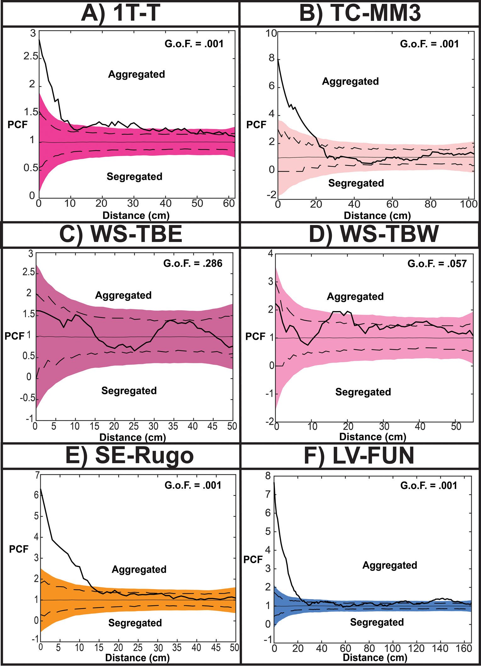
Figure 5. Complete spatial randomness (CSR) results for the beds examined. Colored simulation envelopes are analytical global envelopes (AGE), dotted lines are pointwise simulation envelopes, thick black line is summary statistic value. A,B, Tribrachidium on 1T-T and TC-MM3 show aggregation at short scales. C, Tribrachidium on WS-TBE are spatially random. D, Tribrachidium on WS-TBW are aggregating from 15 to 22 cm. E,F, Rugoconites on SE-Rugo and Obamus on LV-FUN both display aggregated distributions. GoF, goodness-of-fit.

Figure 6. Heterogenous Poisson (HP) results for the beds examined. Colored simulation envelopes are analytical global envelopes (AGE), dotted lines are pointwise simulation envelopes, thick black line is summary statistic value. A, Tribrachidium on 1T-T does not fit the HP null model, while those on B–D TC-MM3, WS-TBE, and WS-TBW were best fit to the HP null model, implying spatial heterogeneity. E,F, Rugoconites on SE-Rugo and Obamus on LV-FUN both do not fit the HP null model. GoF, goodness-of-fit.

Figure 7. Thomas cluster (TC) and double Thomas cluster (DTC) null model results. Colored simulation envelopes are analytical global envelopes (AGE), dotted lines are pointwise simulation envelopes, thick black line is summary statistic value. Note that only communities that were aggregated could be tested against a TC or DTC null model. A–F, All three of the aggregated populations were fit to both a TC and DTC. GoF, goodness-of-fit.
Rugoconites
The population of Rugoconites on SE-Rugo is aggregated (Figs. 5E, 6E). Both a TC and a DTC provide good fit to the observed pattern, with DTC as the best fit (best-fit pd = 0.797) (Fig. 7B,D, Table 2). The heterogenous models (HP, HPTC, or HPDTC) were not good fits for the Rugoconites population on SE-Rugo.
Obamus
On LV-FUN, Obamus are strongly aggregated and have good fit to both TC and DTC models, with the TC null model as the best fit (best-fit pd = 0.556) (Figs. 5F, 6F, 7C,F, Table 2). Strong aggregation was determined by examining the initial aggregation values calculated using a CSR null model, revealing a PCF value of 7.66, significantly outside the AGE (Fig. 5F). The heterogenous models (HP, HPTC, or HPDTC) were not good fits for the Obamus population on LV-FUN.
Discussion
Each taxon examined here, and specifically Tribrachidium, displays different population densities and distributions across the surfaces at NENP (Table 1). Tribrachidium has varying distributions throughout NENP, ranging from isolated individuals, to random distributions on multiple heterogenous surfaces, to an aggregated single-generation population on surface 1T-T. Varying spatial distribution patterns have been documented among both modern organisms (e.g., the European barnacle Chthamalus stellatus has both random and aggregated patterns; Guy-Haim et al. Reference Guy-Haim, Rilov and Achituv2015), and Ediacaran taxa (e.g., Aspidella specimens from three surfaces excavated from both the Olenek Uplift and the White Sea; Mitchell et al. Reference Mitchell, Bobkov, Bykova, Dhungana, Kolesnikov, Hogarth, Liu, Mustill, Sozonov, Rogov, Xiao and Grazhdankin2020).
The aggregated distribution contrasts with previous spatial analytical results yielding random distributions for Tribrachidium on 1T-T (Hall et al. Reference Hall, Droser, Gehling and Dzaugis2015). This disparity is a function of the application of different methods; Hall et al. (Reference Hall, Droser, Gehling and Dzaugis2015) used nearest-neighbor analysis, which as they note was hampered by irregularly shaped study areas and edge effects. Additionally, nearest-neighbor analysis is limited to the largest nearest-neighbor distance, so it can normally only handle scales much smaller than spatial scales captured by PCF. The aggregated distribution of Tribrachidium on 1T-T is an outlier compared with the other Tribrachidium surfaces examined here. It is not uncommon for generally solitary and/or randomly distributed marine sessile invertebrates to be densely populated if advantageous environmental conditions permit (Schmidt Reference Schmidt1982; Rossi and Snyder Reference Rossi and Snyder2001); however, the specific settlement conditions that enabled Tribrachidium to be very abundant and dense on 1T-T (density = 28 individuals/m2) are unknown. Both settlement conditions or post-settlement environmental filtering could allow for strong aggregation, and it is not possible to distinguish between the two with the methods used here. Tribrachidium on TC-MM3, WS-TBE, and WS-TBW are best fit to an HP null model, implying the presence of an external effect, such as environmental heterogeneity, on their distribution. The cause of this heterogeneity is unknown, but did not impact the settlement or life span of the 1T-T Tribrachidium population. It could be that there were originally dense populations of Tribrachidium on TC-MM3, WS-TBE, and WS-TBW but that organisms died over time as a result of post-settlement filtering.
At NENP, Tribrachidium is found on 12 surfaces (from two facies) exhibiting variable community development, diversity, paleobathymetry, and microbial mat maturity. Tribrachidium has been found as solitary individuals on three of those surfaces (STC-AB, 1T-LS, LV-FUN; Table 1), implying that the aggregation found on 1T-T is not likely a function of Tribrachidium being spatially limited in its dispersal or requiring conspecifics nearby for reproductive purposes, as is the case for some modern invertebrates (Pawlik Reference Pawlik1992; Rodríguez et al. Reference Rodríguez, Ojeda and Inestrosa1993; Davis and Campbell Reference Davis and Campbell1996). Reproductive method can play a role in the dispersal of an organism even if said organism does not need to be near conspecifics for post-settlement reproduction. While it is possible that Tribrachidium had multiple modes of reproduction resulting in different dispersal patterns, previous work determined that they likely had a seasonal or opportunistic sexual reproductive method, with clear size cohorts on NENP surfaces (Hall et al. Reference Hall, Droser, Gehling and Dzaugis2015). Similarly, Zakrevskaya (Reference Zakrevskaya2014) found a single size cohort of Tribrachidium at a White Sea locality. Among modern marine invertebrates, there is a positive relationship between the supply of larvae and settlement rates that operates over multiple spatial scales (0–100 m, 100–1000 m, and 100–1000 km; Jenkins Reference Jenkins2005). An organism reproducing via opportunistic sexual reproduction could secure a substrate with a preexisting low species diversity and populate the surface with high abundance. This method of dispersal could be detected as aggregation, as it is a function of increased density, due to the nature of SPPA. If more points are added to a “study area,” then it is more likely that the average neighborhood density (i.e., the number of points separated by a distance [r]) will have a higher value than that of a random distribution, thus resulting in an aggregated pattern (Wiegand and Moloney Reference Wiegand and Moloney2014). The combination of weak aggregation and higher density compared with Rugoconites or Obamus (1T-T: 28 individuals/m2; SE-Rugo:10 individuals/m2; LV-FUN: 5 individuals/m2), supports the hypothesis that the distribution of Tribrachidium on 1T-T is likely a function of preferred settlement conditions or low post-settlement environmental filtering (Table 1).
The fact that different populations of Tribrachidium exhibit various spatial distributions and densities may also further support that Tribrachidium was able to live and thrive in a wide variety of environmental and ecological settings. While the process leading to the densely populated and aggregated distribution of Tribrachidium on 1T-T is unknown, an opportunistic life strategy could secure a substrate with high availability in ecospace (Hall et al. Reference Hall, Droser, Gehling and Dzaugis2015).
These results may also have implications for our understanding of other ecological aspects of Tribrachidium. Using computational fluid dynamics, Rahman et al. (Reference Rahman, Darroch, Racicot and Laflamme2015) found that modeled fluid flow around a Tribrachidium supported the conclusion that Tribrachidium was a passive suspension feeder, but their simulations only modeled flow around a single Tribrachidium fossil. The authors suggest that a dense community would have helped enable a consistent flow of suspended nutrients. A similar study that modeled fluid flow around aggregated Ernietta fossils found that a gregarious lifestyle would have aided suspension feeding for those organisms (Gibson et al. Reference Gibson, Rahman, Maloney, Racicot, Mocke, Laflamme and Darroch2019), which could similarly hold for Tribrachidium, despite differences in morphology. Based on an observational study of Tribrachidium morphology, Ivantsov and Zakrevskaya (Reference Ivantsov and Zakrevskaya2021) instead proposed that Tribrachidium fed using a more active feeding style, moving food particles along branched grooves, interpreted based on the “frill” commonly preserved on White Sea specimens. Modeling fluid flow around aggregated and randomly distributed Tribrachidium may help constrain whether their presumed feeding style also played a role in their spatial distributions, or whether certain feeding styles can be ruled out based on the existence of both aggregated and randomly distributed populations.
As previously noted, Rugoconites occurs on multiple surfaces with differing diversity, facies, and microbial mat maturity (Hall et al. Reference Hall, Droser and Gehling2018). Rugoconites occurs as low abundance and density populations on 11 beds at NENP (Table 1). Rugoconites on SE-Rugo was best fit to a DTC model, suggesting that these organisms were distributed in clusters of clusters (best-fit pd = 0.797) (Fig. 7B,E). Aggregation, in a general ecological sense, implies that either a biological or environmental factor is affecting the distribution of an organism (Carlon and Olson Reference Carlon and Oslon1993; Karlson et al. Reference Karlson, Hughes and Karlson1996; He and Legendre Reference He and Legendre2002; Franklin and Santos Reference Franklin and Santos2010; Lin et al. Reference Lin, Chang, Yang, Wang and Sun2011; Ambroso et al. Reference Ambroso, Gori, Dominguez-Carrió, Gill, Berganzo, Teixidó, Greenacre and Rossi2013; Carrer et al. Reference Carrer, Castagneri, Popa, Pividori and Lingua2018). The intensity of aggregation detected on SE-Rugo is stronger than on 1T-T's Tribrachidium population (initial PCF values for 1T-T: 2.84; SE-Rugo: 6.32) (Fig. 5A,E); however, the population density of Rugoconites is still high compared with other taxa at Nilpena (Droser et al. Reference Droser, Gehling, Tarhan, Evans, Hall, Hughes, Hughes, Dzaugis, Dzaugis, Dzaugis and Rice2019; Table 1). This high density implies that while the aggregation is not solely a function of density-dependent processes, Rugoconites is possibly another example of an opportunistic or seasonally reproducing organism having advantageous settlement conditions or low post-settlement mortality rates. Hall et al. (Reference Hall, Droser and Gehling2018), using size–frequency distributions from surfaces including SE-Rugo, determined that Rugoconites at NENP likely reproduced sexually.
Benthic marine invertebrates that reproduce sexually can exhibit strong aggregation related to dispersal and/or settlement mechanisms. Specifically, three methods result in strong aggregation: habitat-selective larval stages, short-lived/dispersed larval stages, and/or a preference for being near conspecifics (Carlon and Olson Reference Carlon and Oslon1993; Lesneski et al. Reference Lesneski, D'Aloia, Fortin and Buston2019). While Rugoconites is more common in the ORS Facies, it is found in numerous environments with no apparent preference for substrate, suggesting that a selective larval stage is unlikely. Most benthic invertebrates need to be near a conspecific to reproduce sexually, whether the distance is centimeters, millimeters, or kilometers in scale, although, there are taxa with reproductive ranges that are over thousands of kilometers in scale (Davis and Campbell Reference Davis and Campbell1996; Takabayashi et al. Reference Takabayashi, Carter, Lopez and Hoegh-Guldberg2002; Neuman et al. Reference Neuman, Wang, Busch, Friedman, Gruenthal, Gustafson, Kushner, Stierhoff, Vanblaricom and Wright2018; Rodriguez-Perez et al. Reference Rodriguez-Perez, Sanderson, Møller, Henry and James2020). The specific reproductive range of Rugoconites is unknown; however, the common occurrence of single or dispersed pairs of Rugoconites on surfaces is not consistent with larval stages settling in locations relatively near conspecifics. The occurrence of solitary Rugoconites shows that they do not necessarily need to be near conspecifics such as certain species of barnacles or oysters (Rodríguez et al. Reference Rodríguez, Ojeda and Inestrosa1993; Rodriguez-Perez et al. Reference Rodriguez-Perez, Sanderson, Møller, Henry and James2020).
Another possible cause of the aggregation of the Rugoconites on SE-Rugo is short dispersal/short-lived larval stage. Certain modern taxa, such as the soft coral Alcyonium acaule, have rapid-settling larvae produced via surface brooding (Ambroso et al. Reference Ambroso, Gori, Dominguez-Carrió, Gill, Berganzo, Teixidó, Greenacre and Rossi2013). These corals have dense aggregated distributions but also a large ecological range, populating extensive portions of the Mediterranean Sea (Ambroso et al. Reference Ambroso, Gori, Dominguez-Carrió, Gill, Berganzo, Teixidó, Greenacre and Rossi2013). However, examining dispersal limitations of an organism preserved on a surface that is only 3.6 m2 is speculative and should be undertaken with caution. It is possible that Rugoconites, like numerous modern marine invertebrates, could reproduce both sexually and asexually. The aggregation of Rugoconites on SE-Rugo could result from unknown ecological or biological factor(s) that made the SE-Rugo surface ideal for settlement or a lack of post-settlement environmental filtering.
In contrast to Rugoconites and Tribrachidium, Obamus exhibits strong aggregation (best fit to a TC model; best-fit pd = 0.556), relatively low population density (5 individuals/m2), and a more selective environmental distribution. One possible explanation for this distribution is asexual reproduction. Another Ediacaran taxon, albeit from the older Avalon Assemblage, that fits a DTC is Fractofusus, which has been determined to have reproduced via stolons (Mitchell et al. Reference Mitchell, Kenchington, Liu, Matthews and Butterfield2015). There is no evidence at NENP of stolons in relation to Obamus, despite exceptional preservation on surfaces such as LV-FUN and TB-ARB, and the spatial scale for Obamus of 20 cm is significantly larger than those in which stoloniferous reproduction occurs (Mitchell et al. Reference Mitchell, Kenchington, Liu, Matthews and Butterfield2015). Despite evidence for quantitatively high intraspecific aggregation, no individuals have been found with edges touching, unlike several other sessile organisms at NENP, such as Aspidella or less commonly Tribrachidium (Hall et al. Reference Hall, Droser, Gehling and Dzaugis2015; Tarhan et al. Reference Tarhan, Droser, Gehling and Dzaugis2015b). The lack of touching among the hundreds of Obamus examined here suggests that asexual fission or budding is unlikely.
Instead, we propose that the selective nature of Obamus requires a dispersal mechanism that allows for some level of habitat preference. Previous studies of Obamus have noted its affinity for locations of mature microbial mat but no preference for mat type (Dzaugis et al. Reference Dzaugis, Evans, Droser, Gehling and Hughes2018; Droser et al. Reference Droser, Evans, Tarhan, Surprenant, Hughes, Hughes and Gehling2022). While pelagic larval stages are the most common type of dispersal for sessile benthic marine invertebrates, other reproductive strategies can result in habitat or range restrictions. In modern ecosystems, certain sponges have short dispersal ranges based on a combination of asexual budding and habitat preference that result in aggregated patterns (Lesneski et al. Reference Lesneski, D'Aloia, Fortin and Buston2019). As was the case with Rugoconites, it is imprudent to attempt to predict the dispersal range of an organism using a surface limited to 22.4 m2, when modern dispersal can range from centimeters to kilometers in scale (Jenkins Reference Jenkins2005).
While an asexual model cannot be fully ruled out, the distribution of Obamus is also consistent with sexual reproduction. Selective larval stages are common among modern marine invertebrates that reproduce sexually, with planktonic larvae that are either transported or actively swim for days to months, navigating at small scales in order to secure a preferred substrate (Carlon and Olson Reference Carlon and Oslon1993; Manríquez and Castilla Reference Manríquez and Castilla2007; Maldonado and Riesgo Reference Maldonado and Riesgo2008; Denley et al. Reference Denley, Metaxas and Short2014; Chase et al. Reference Chase, Dijkstra and Harris2016; Wangensteen et al. Reference Wangensteen, Turon, Placin, Rossi, Bramanti, Gori and Orejas2016). These data do not suggest a swimming larval phase for Obamus; however, Obamus was not limited in its environmental dispersal range, occurring in two separate facies at NENP, reflecting environments between fair weather and storm wave base to a sub–wave base upper canyon fill (Droser et al. Reference Droser, Gehling, Tarhan, Evans, Hall, Hughes, Hughes, Dzaugis, Dzaugis, Dzaugis and Rice2019). Obamus has not been found as a solitary individual on any surface at NENP, implying that at some scale, Obamus needed to be near conspecifics or had limited dispersal ranges. This, combined with a preference for specific substrates, could be responsible for the strong aggregation found on LV-FUN.
Tribrachidium is spatially variable, similar to Aspidella specimens from the Olenek Uplift and White Sea of Russia (although the types of variable spatial patterns differed; Mitchell et al. Reference Mitchell, Bobkov, Bykova, Dhungana, Kolesnikov, Hogarth, Liu, Mustill, Sozonov, Rogov, Xiao and Grazhdankin2020). Aggregation, recorded in all three taxa here, was documented in Funisia and Parvancorina populations collected from the Ediacara Hills, South Australia (Coutts et al. Reference Coutts, Bradshaw, García-Bellido and Gehling2018; Mitchell et al. Reference Mitchell, Bobkov, Bykova, Dhungana, Kolesnikov, Hogarth, Liu, Mustill, Sozonov, Rogov, Xiao and Grazhdankin2020). The prevalence of aggregation for many of the White Sea taxa is consistent with modern marine benthic invertebrates, whose populations are often aggregated as a result of reproductive or environmental controls (e.g., Schmidt Reference Schmidt1982; Keough Reference Keough1984; Carlon and Olson Reference Carlon and Oslon1993; Rodríguez et al. Reference Rodríguez, Ojeda and Inestrosa1993; Miron et al. Reference Miron, Boudreau and Bourget1999; Manríquez and Castilla Reference Manríquez and Castilla2007; Ambroso et al. Reference Ambroso, Gori, Dominguez-Carrió, Gill, Berganzo, Teixidó, Greenacre and Rossi2013; Hooper and Eichhorn Reference Hooper and Eichhorn2016; Lesneski et al. Reference Lesneski, D'Aloia, Fortin and Buston2019; De los Ríos and Carreño Reference De los Ríos and Carreño2020; Rodriguez-Perez et al. Reference Rodriguez-Perez, Sanderson, Møller, Henry and James2020). Furthermore, Charniodiscus and Fractofusus from the Avalon Assemblage and Ernietta from the Nama Assemblage in Namibia (Gibson et al. Reference Gibson, Rahman, Maloney, Racicot, Mocke, Laflamme and Darroch2019, Reference Gibson, Darroch, Maloney and Laflamme2021; Mitchell et al. Reference Mitchell, Harris, Kenchington, Vixseboxse, Robers, Clark, Dennis, Liu and Wilby2019) have been shown to exhibit aggregation, indicating that this spatial pattern was present, or even common, throughout the Ediacara Biota.
While the pattern of aggregation is common throughout Ediacaran assemblages, the processes leading to these patterns differ by assemblage and taxa. In the Avalon Assemblage, spatial patterns are driven by random dispersal processes, while in the White Sea Assemblage, the dispersal method and environmental factors both play a role in distribution (Mitchell et al. Reference Mitchell, Kenchington, Liu, Matthews and Butterfield2015, Reference Mitchell, Harris, Kenchington, Vixseboxse, Robers, Clark, Dennis, Liu and Wilby2019, Reference Mitchell, Bobkov, Bykova, Dhungana, Kolesnikov, Hogarth, Liu, Mustill, Sozonov, Rogov, Xiao and Grazhdankin2020). Additionally, among Avalon taxa, spatial patterns and the processes that cause them are relatively consistent across different surfaces, which is not the case for White Sea taxa populations (e.g., the Tribrachidium; Mitchell et al. Reference Mitchell, Harris, Kenchington, Vixseboxse, Robers, Clark, Dennis, Liu and Wilby2019). Finally, patterns in the Nama Assemblage have been reported as being a process of facilitation (Gibson et al. Reference Gibson, Rahman, Maloney, Racicot, Mocke, Laflamme and Darroch2019). However, these observations require further work before any larger spatial ecological trends can be deduced from the three Ediacaran Assemblages.
Conclusions
The reproductive strategies of sessile marine invertebrates are vital to their spatial distributions. With the statistically viable populations examined here, it is possible to determine that different taxa at NENP had variable spatial distributions. These distributions also reflect key aspects of their life histories. In the case of Tribrachidium, we find that populations are best fit to the heterogenous Poisson or double Thomas cluster null models and are driven by either environmental and/or dispersal processes. Rugoconites shows strong aggregation, but occur in low numbers on numerous beds. This pattern could be a function of reproductive methods in combination with settlement location availability at the time of dispersal and/or settlement. Additionally, post-settlement environmental controls could have resulted in the low specimen number on some surfaces. Tribrachidium and, to a lesser extent, Rugoconites are both possible examples of aggregation occurring when conditions were advantageous for dense settlement or outliers resulting from common post-settlement filtering on non-aggregated surfaces. Obamus is an example of a strongly aggregated organism that only occurs with conspecifics and in locations of mature microbial mats. This dispersal process is the first example of a member of the Ediacara Biota that was substrate selective, something commonly found throughout modern invertebrate populations.
Acknowledgments
Thanks are extended to the Department of Environment and Water of the South Australia government and to R. Fargher and J. Fargher for access to the NENP. We acknowledge that this land lies within the Adnyamathanha Traditional Lands. Additionally, we acknowledge that the University of California, Riverside (where the majority of lab work was done) lies within the traditional lands of the Cahuilla, Tongva, Luiseño, and Serrano Peoples. H. McCandless assisted in the logging of TBEW and creation of photogrammetric 3D models. We thank A. Kovalick, A. Rizzo, W. Weyland, and R. Surprenant for their helpful discussions. T. Wiegand provided helpful suggestions and explanations regarding SPPA methodology. Fieldwork was facilitated by P. Dzaugis, I. Hughes, and E. Hughes. N. Tam, G. M. Boan, and M. Figueroa aided in the preparation of this article. This project was funded by the NASA Exobiology Program (NASA grant NNG04GJ42G) to M.L.D., a student research grant from the Society for Sedimentary Geology awarded to P.C.B., a Lerner-Gray Memorial Fund for Marine Research grant from the American Museum of Natural History awarded to P.C.B., a CARES grant from the Geological Society of America awarded to P.C.B., an N. Gary Lane Student Research Award grant from the Paleontological Society awarded to P.C.B, and an NSF/GSA Graduate Student Geoscience grant no. 13053-21, which is funded by NSF Award no. 1949901 awarded to P.C.B. This paper benefited greatly from reviews by E. Mitchell and an anonymous reviewer.
Declaration of Competing Interests
The authors declare no competing interests.
Data Availability Statement
Data available from the Dryad Digital Repository: https://doi.org/10.6086/D1M67C.


