


1. Introduction
It is well known that surfactants can act to produce Marangoni stresses at interfaces that in turn retard the motion and diminish any fluid process advantages in applications. Examples include, but are not limited to: the retardation of rising gas bubbles (or droplets) in a continuous liquid phase that contains surfactants – see recent experiments and theory of Duinevelt (Reference Duinevelt1995), Takemura (Reference Takemura2005) and Palaparthi, Papageorgiou & Maldarelli (Reference Palaparthi, Papageorgiou and Maldarelli2006), and the review by Takagi & Matsumoto (Reference Takagi and Matsumoto2011); the loss of slip in superhydrophobic microchannels structured with gas-filled grooves so that the flow is in the Cassie state – see, for instance, the experiments of Peaudecerf et al. (Reference Peaudecerf, Landel, Goldstein and Luzzatto-Fegiz2017). This loss of mobility in the context of bubble motion was recognized almost a century ago (Bond & Newton Reference Bond and Newton1928), and a consistent explanation of the retardation phenomena has been given by Frumkin & Levich (Reference Frumkin and Levich1947) and Levich (Reference Levich1962), who noted the presence of trace amounts of surfactant impurities in the liquid phase. Briefly, as the bubble rises, surfactant in the bulk diffuses towards the front end and adsorbs kinetically there. It is then swept to the rear of the bubble by surface convection, where the surfactant concentration increases and hence desorbs and diffuses into the bulk. The surface tension at the back is therefore lower than at the front, and a Marangoni stress opposing the flow emerges and causes the observed retardation. The mechanisms are identical in other geometries such as the superhydrophobic channel flows mentioned above.
The physical problem is a complex multiphysics one with many competing effects at work, and useful insight can be gained by considering the rates and relative magnitudes of different mechanisms. The crucial quantities are the rate at which surfactant exchanges kinetically with the interface, the rate of diffusive exchange between the bulk and the interface, the rate of interfacial diffusion of surfactant, and the rate of surface convection of surfactant. When the size of the first three mechanisms is small relative to surface convection, surfactant gradients on the interface are expected to be sizeable and will produce large Marangoni stresses. This leads to the so-called stagnant cap regime and subsequently to the limit of insoluble surfactant where surfactant stays on the interface and does not exchange with the bulk. Studies of the insoluble limit in the case of bubbles are numerous: Palaparthi et al. (Reference Palaparthi, Papageorgiou and Maldarelli2006) give a survey of much of the relevant literature. For more recent work on superhydrophobic channel flows, Peaudecerf et al. (Reference Peaudecerf, Landel, Goldstein and Luzzatto-Fegiz2017), Baier & Hardt (Reference Baier and Hardt2021), Crowdy (Reference Crowdy2021a,Reference Crowdyb) and Mayer & Crowdy (Reference Mayer and Crowdy2022) are useful references.
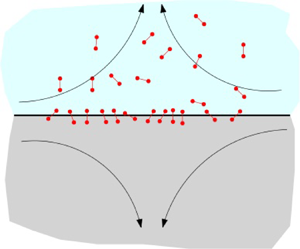
To motivate the mathematical models solved here, consider two immiscible fluids experiencing a linear extensional flow and separated by a flat interface; soluble surfactant is present in the upper region (fluid 2) while the lower region (fluid 1) is taken to be free of surfactants (they are insoluble to the lower fluid). A schematic is given in figure 1. Langmuir kinetics describe the exchange of surfactant between the interface and the liquid sublayer next to it. Defining  $j$ to be the kinetic flux of surfactant, we have
 \begin{equation} j = b c_s (\varGamma_\infty -\varGamma) - a \varGamma,\end{equation}
where  $a$ and $b$ are respectively the desorption and adsorption kinetic constants, $c_s$ is the sublayer concentration of surfactant, and $\varGamma _\infty$ is the maximum packing concentration density on the interface. At equilibrium, $c_0$ is defined to be the surfactant concentration in the bulk of fluid 2, and setting $j=0$ in (1.1) gives the equilibrium interfacial surfactant concentration
 \begin{equation} \varGamma_0=\varGamma_{\infty}k/(1+k),\end{equation}
where  $k=bc_0/a$ is a measure of the dimensionless initial surfactant concentration in the bulk. The reduction in surface tension is modelled by the Langmuir isotherm
 \begin{equation} \sigma= \sigma_c + \beta \varGamma_\infty \log (1-\varGamma/\varGamma_\infty), \quad \beta = RT, \end{equation}
where  $\sigma _c$ is the clean surface tension value. Combining (1.3) at equilibrium with (1.2) gives $\sigma _c-\sigma _0=-\beta \log (1-\varGamma _0/\varGamma _\infty ) =\beta \varGamma _\infty \log (1+k)$, where $\sigma _0$ is the surface tension value at equilibrium. This expression shows that the ratio $a/b$ acts as a surface activity measure of the surfactant. For a given equilibrium concentration $c_0$, smaller values of $a/b$ imply larger values of $k$ and hence greater reductions in equilibrium tension.

Figure 1. A linear extensional flow near the interface between two viscous fluids. A surfactant with surface concentration  $\varGamma (x,t)$, insoluble to a lower fluid of viscosity $\mu _1$ but soluble to an upper fluid of viscosity $\mu _2$, diffuses in the upper fluid, where surfactant molecules have concentration $c(x,y,t)$ and are in fast kinetic exchange with the interface. The surface tension on the interface is $\sigma (x,t)$.
The relative magnitudes of the different physical mechanisms involved can now be described. For a detailed description of such order-of-magnitude estimates in the case of bubble motion, the reader is referred to Wang, Papageorgiou & Maldarelli (Reference Wang, Papageorgiou and Maldarelli1999, Reference Wang, Papageorgiou and Maldarelli2002) and Palaparthi et al. (Reference Palaparthi, Papageorgiou and Maldarelli2006).
The transport of surfactant by diffusion from the bulk to the sublayer (and vice versa) is given by  $D\,\partial c/\partial y$ in our geometry, where $D$ is the diffusion coefficient of the surfactant, and $c(x,y,t)$ is the bulk concentration – see figure 1. For a typical length scale $L$, the diffusive transport scales with $Dc_0/L$. Here, $L$ will be taken to be the linear dimension of the initial distribution of surfactant, e.g. a compactly supported patch of surfactant in the bulk and adjacent to the interface of extent $L$ (see later). Diffusion of surfactant on the interface scales with $D_s({\rm \Delta} \varGamma )/L^2$, where $D_s$ is the surface diffusion, and ${\rm \Delta} \varGamma$ is the difference between the maximum and minimum surfactant concentrations. On isolating the positive terms in (1.1), the rate of adsorption of surfactant is found to be of order $b c_0\varGamma _\infty$, or $ak\varGamma _\infty$, while the negative terms give the rate of desorption to be $bc_0\varGamma _0+a\varGamma _0=ak\varGamma _\infty$. Defining $U_0$ to be a typical velocity, the convective flux of surfactant at the interface can be estimated to be $\varGamma _0 U_0/L$. The following three regimes emerge (see Palaparthi et al. (Reference Palaparthi, Papageorgiou and Maldarelli2006) for more details).
The stagnant cap regime: this is achieved when the rate of diffusive flux, or adsorption/desorption from the interface to the bulk, is small compared to the surface convection. The surfactant behaves as if it were insoluble, and stagnant caps can form. The ratio of diffusive flux to surface convection is  $(Dc_0/L)/(\varGamma _0 U_0/L)=\chi (k+1)/Pe$, where $\chi =aL/b\varGamma _\infty$, and $Pe=U_0 L/D$ is the bulk Péclet number, while the rate of adsorption/desorption to surface convection is $ak\varGamma _\infty /(\varGamma _0 U_0/L)=Bi (1+k)$, where $Bi=aL/U_0$ is the Biot number. Hence the stagnant cap regime is expected when $\chi (k+1)/Pe\ll 1$ or $Bi (1+k)\ll 1$.
The uniformly retarded regime: in this case, there is a balance between diffusive transport, adsorption/desorption and surface convection, a regime that is characterized by  $\chi (k+1)/Pe={O}(1)$ and $Bi(1+k)={O}(1)$. The term ‘uniformly retarded’ is used to differentiate the phenomena from the stagnant cap case where there is a region on the surface that is free of surfactant and a region that is fully covered. Mathematically, this is the most complicated case due to the full coupling and retention of all terms in the equations. Physically, the resulting drag will be less than that in the stagnant cap case, and direct numerical simulations are usually necessary.
The remobilization regime: in this regime there is much faster kinetic and bulk diffusive exchange with the interface as compared to the convection of surfactant along the interface. Physically, the latter effect does not have the ability to sweep surfactant to one end and to induce a large difference in surface concentration  ${\rm \Delta} \varGamma$ that would result in a retarding Marangoni stress. The value of $\varGamma$ increases, but ${\rm \Delta} \varGamma$ remains small, hence the Marangoni stress is reduced. Remobilization takes place when $\chi (k+1)/Pe\gg 1$ and $Bi (1+k)\gg 1$. The case of diffusion-limited transport, namely $Bi\to \infty$ and $\chi (k+1)/Pe={O}(1)$, has been considered, in the case of rising bubbles, by Wang et al. (Reference Wang, Papageorgiou and Maldarelli1999, Reference Wang, Papageorgiou and Maldarelli2002) for both small and order-one Reynolds numbers, where remobilization was clearly shown theoretically. This paper considers the analogous limit for an extensional flow problem near a flat interface.
Importantly, for the first time, this paper constructs analytical solutions to a class of such problems. The mathematics involved is underpinned by recent work by Crowdy (Reference Crowdy2021a,Reference Crowdyb) that has lent new analytical insights into the dynamics of insoluble surfactant on a planar free surface at zero capillary and Reynolds numbers. In that work, a key role is played by complex partial differential equations (PDEs) of Burgers type that emerge from a complex variable reformulation of the physical problem. In particular, Crowdy (Reference Crowdy2021a) has given a class of explicit, time-evolving solutions for the evolution of the surfactant concentration on a planar free surface in the presence of a linear background strain akin to that at the rear of a rising bubble. At long times, the solutions tend to, but never quite reach, a stagnant cap equilibrium where, in the absence of diffusion or reaction effects, the surfactant piles up onto an immobilized portion of the interface. Mathematically, this manifests in the analysis as two square root branch points of a relevant analytic function approaching the interface from an unphysical region of the complex plane. The two square root branch points correspond physically to the edges of the stagnant cap.
Reaction kinetics have also been incorporated into the mathematical approach based on PDEs of complex Burgers type (Crowdy Reference Crowdy2021a), and exact solutions are available in that case too. This simple model assumes that surfactant sublimates off the interface according to a first-order reaction model. It admits no mechanism for re-adsorption of surfactant to the interface, however, and the model is found simply to destroy the stagnant cap equilibrium, as expected. It is this deficiency that the work in the present paper eliminates. It is worth pointing out that Bickel (Reference Bickel2019) studied the same first-order reaction model as Crowdy (Reference Crowdy2021a) using an approach based on Hilbert transforms, and without recognizing the connection to the complex Burgers equation, but has since made further advances (Bickel & Detcheverry Reference Bickel and Detcheverry2022) in light of the connection to Burgers-type PDEs unveiled by Crowdy (Reference Crowdy2021a,Reference Crowdyb). The theoretical connection therefore appears to be a fruitful one, and this matter is surveyed again later in § 12.
The present paper shows that the analytical approach set out in Crowdy (Reference Crowdy2021a,Reference Crowdyb) based on PDEs of complex Burgers type can be extended even further, both to a two-fluid scenario and, even more, to the case where there is steady fast reactive exchange of surfactant on and off the interface. In this study, attention is restricted to the situation where there is reactive exchange of surfactant between the interface and the upper liquid phase, but where the surfactant remains insoluble in the lower liquid; the theory extends to other scenarios, however. In the limit of diffusion-limited transport where fast kinetics control adsorption/desorption (that is, in the limit  $Bi\to \infty$) with a diffusive surfactant concentration field in the upper liquid phase, it is demonstrated here that the stagnant cap is remobilized as explained earlier, and consequently results in generally lower Marangoni stresses (Palaparthi et al. Reference Palaparthi, Papageorgiou and Maldarelli2006). Since this generalized model now allows for two-way exchange of surfactant on and off the interface, an equilibrium now survives and, as will be shown here, is characterized by gentler gradients of interfacial slip and, indeed, interface remobilization. By generalizing the complex variable methods of Crowdy (Reference Crowdy2021a,Reference Crowdyb), all this is demonstrated in explicit analytical form, a quite remarkable circumstance given the complexity of this multiphysics system.
The structure of the paper is as follows. Section 2 provides the governing equations for general surfactant characteristics. Section 3 gives the non-dimensionalization, and § 4 discusses the dilute limit in the presence of fast reaction kinetics. The complex variable formulation is provided in § 5, leading to a complex Burgers-type equation in § 6. It is also shown there, by means of a complex generalization of the classical Cole–Hopf transformation, that the full nonlinear problem considered here can be linearized at arbitrary surface Péclet number. Steady equilibria for arbitrary values of the surface Péclet number, that is, with any given amount of surface diffusion, are given in § 7 in terms of parabolic cylinder functions. The analytical approach allows for surface diffusion to be switched off completely, leading to theoretical isolation of the effects on remobilization of the fast reactive exchange alone, and this extreme case is analysed in § 8; the structure of the steady-state solutions is then much simpler. Indeed, in the absence of surface diffusion, it is possible to solve analytically for the time evolution of the solutions: in § 9 a complex version of the method of characteristics is shown to lead to an implicit solution for arbitrary initial conditions. A special class of explicit time-evolving solutions tending, at large times, to the remobilized equilibria found in § 8 is then studied in § 10. After a discussion of the physical relevance of the mathematical model in § 11, the paper closes with a discussion in § 12.
2. Mathematical formulation
Consider an  $(x,y)$-plane where a fluid with viscosity $\mu _1$ lies in the lower half-plane $y < 0$ (region 1) and another of viscosity $\mu _2$ lies in the upper half-plane $y> 0$ (region 2), as indicated schematically in figure 1. An infinite interface along $y=0$ having surface tension $\sigma (x,t)$ is assumed to be laden with surfactant with concentration $\varGamma (x,t)$. Following Crowdy (Reference Crowdy2020, Reference Crowdy2021a), it is assumed that a capillary number based on a clean-flow surface tension value is negligible so that the normal stress balance can be ignored and the interface can be taken to remain undeflected from $y=0$.
Both fluids are taken to be in the Stokes regime so that the velocity fields  ${\boldsymbol{u}}_j = (u_j,v_j)$ for $j=1,2$ satisfy
 \begin{equation} \mu_j\,\nabla^2 {\boldsymbol{u}}_j = \boldsymbol{\nabla} p_j, \quad \boldsymbol{\nabla} \boldsymbol{\cdot} {\boldsymbol{u}}_j = 0, \end{equation}
in their respective regions, where  $p_j(x,y,t)$ is the fluid pressure in region $j$. The boundary conditions on $y=0$ are
 \begin{equation} u_1 = u_2, \quad v_1 = v_2= 0, \quad \mu_1\, \frac{\partial u_1 }{\partial y} - \mu_2\, \frac{\partial u_2 }{\partial y} ={-} \frac{\partial \sigma }{\partial x},\end{equation}
which ensure, respectively, that fluid velocities are continuous across the interface, that the latter is a streamline, and that any net fluid shear stress across the interface is balanced by a Marangoni stress caused by the surface tension variation. Since we are interested in stagnant caps, in the far field in both fluid regions, a pure extensional flow is assumed with strain rate  $\dot \gamma _0$ of the form
 \begin{equation} (u_j,v_j) \sim (-\dot \gamma_0 x, \dot \gamma_0 y), \quad j=1,2.\end{equation}
This far-field behaviour is consistent with the velocity boundary conditions in (2.2a–c). At large distances from the origin, however, the large velocities associated with such a flow are not consistent with the assumption of Stokes flow, and corrections will be needed there; but the focus here is on the vicinity of the origin towards which, in the presence of such a linear extensional flow, any surfactant on the interface is expected to be swept. Then, in the absence of surface diffusion or surfactant exchange with the bulk, a stagnant cap of surfactant, i.e. an immobilized region of the interface, will form (Palaparthi et al. Reference Palaparthi, Papageorgiou and Maldarelli2006; Crowdy Reference Crowdy2021a). Indeed, Crowdy (Reference Crowdy2021a) has recently given an analytical description of the time-dependent formation of such stagnant caps in the single-phase scenario where the upper region is taken to be a constant pressure zone. Several previous theoretical studies have examined such a two-dimensional single-fluid system with a view to understanding the transition region at the edge of a stagnant cap (Harper Reference Harper1992) and surfactant spreading (Jensen Reference Jensen1995).
Suppose that  $L$ is a typical length scale associated with the support of the surfactant on the interface set by initial conditions, and let $\varGamma _\infty$ be the maximum surface packing concentration. According to (1.3), the Langmuir equation of state is
 \begin{equation} \sigma= \sigma_c + \beta \varGamma_\infty \log (1-\varGamma/\varGamma_\infty), \quad \beta = RT.\end{equation}
As already mentioned, a capillary number based on  $\sigma _c$ is sufficiently small that surface deflection can be ignored and the interface assumed to be flat, occupying the line $y=0$ at all times (Crowdy Reference Crowdy2020, Reference Crowdy2021a).
The surfactant is taken to be soluble to the upper fluid phase but insoluble to the lower fluid phase. The bulk concentration of surfactant molecules in region 2 is denoted by  $c(x,y,t)$ and is governed by the advection diffusion equation
 \begin{equation} \frac{\partial c }{\partial t} +{\boldsymbol{u}}_2\boldsymbol{\cdot} \boldsymbol{\nabla} c = D\,\nabla^2 c(x,y,t), \end{equation}
where  $D$ is the diffusion coefficient of the surfactant molecules in region 2. Since the aim is to study the possible dynamical effects of small amounts of ambient surfactant molecules not fed by any far-field source, it is assumed that any non-zero concentration of surfactant is localized in the sense that
 \begin{equation} c(x,y,t) \to 0 \quad {\rm as}\ |\boldsymbol{x}| \to \infty. \end{equation}
 To represent surfactant going on and off the interface, we introduce the kinetic flux  $j$ of surfactant onto the interface as
 \begin{equation} j = b c_s (\varGamma_\infty -\varGamma) - a \varGamma,\end{equation}
where  $a$ is the desorption coefficient, $b$ is the adsorption coefficient, and
 \begin{equation} c_s = c(x,0,t) \end{equation}
is the so-called sublayer concentration (Palaparthi et al. Reference Palaparthi, Papageorgiou and Maldarelli2006). Conservation of surfactant requires that
 \begin{equation} D \left.\frac{\partial c }{\partial y} \right|_{y=0} = j.\end{equation}
On the interface at  $y=0$, the surfactant evolution equation has the form
 \begin{equation} \frac{\partial \varGamma }{\partial t} + \frac{\partial (\varGamma \mathcal{U}) }{\partial x} = D_s\,\frac{\partial^2 \varGamma }{\partial x^2} + j, \end{equation}
where  $\mathcal {U}(x,t) = u(x,0,t)$ is the surface slip velocity, and $D_s$ is the surface diffusion coefficient. For consistency with (2.6), we also assume that the far-field interface is clean,
 \begin{equation} \varGamma(x,t) \to 0 \quad\text{as } |x| \to \infty,\end{equation}
which means that any surfactant on the interface is also localized.
3. Non-dimensionalization
The velocity scale given by
 \begin{equation} \mathcal{U}_0 = \frac{\beta \varGamma_\infty }{2 (\mu_1 + \mu_2)}\end{equation}
turns out to be the most convenient for this analysis; it is the natural two-phase analogue of the single-phase velocity scale used by Crowdy (Reference Crowdy2021a,Reference Crowdyb). It is also a natural choice of velocity scale when a given initial distribution of surfactant simply spreads on the interface in the absence of any external flow. Velocities will be scaled with respect to this quantity, lengths with respect to  $L$, time with respect to $L/\mathcal {U}_0$, fluid pressures with respect to $\mathcal {U}_0 \mu _i/L$, bulk concentrations with respect to $c_0$, and surface concentrations with respect to $\varGamma _\infty$.
While  $\mathcal {U}_0$ does not depend on the externally applied flow, an alternative velocity scale for this problem is $\mathcal {U}_0^*=\dot {\gamma }_0 L$. The latter could have been used in the non-dimensionalization, but as discussed further in § 11, $\mathcal {U}_0$ can be used to evaluate the magnitude of the external flow and hence key quantities such as the Biot and Péclet numbers.
The flux balance equation (2.9) gives
 \begin{equation} D\,\frac{\partial c }{\partial y} = b c_s (\varGamma_\infty -\varGamma) - a \varGamma,\end{equation}
which, using primes to denote non-dimensional quantities, is
 \begin{equation} \frac{D c_0 }{L}\,\frac{\partial c' }{\partial y'} =a \varGamma_\infty \left( \frac{b }{a}\,c_0 c_s' (1-\varGamma') - \varGamma' \right).\end{equation}
Equation (3.3) can be written as
 \begin{equation} \frac{D c_0 }{\mathcal{U}_0 \varGamma_\infty}\, \frac{\partial c' }{\partial y'} =\frac{a L }{\mathcal{U}_0} \left( \frac{b }{a}\,c_0 c_s' (1-\varGamma') - \varGamma' \right), \quad {\rm on}\ y=0. \end{equation}
After dropping primes on all variables, (3.4) becomes
 \begin{equation} \alpha \left.\frac{\partial c }{\partial y} \right|_{y=0} = Bi ( k c_s (1-\varGamma) - \varGamma ),\end{equation}
where we have introduced the non-dimensional parameters
 \begin{equation} Bi = \frac{a L }{\mathcal{U}_0}, \quad k = \frac{b c_0 }{a}, \quad \alpha = \frac{D c_0 }{\mathcal{U}_0 \varGamma_\infty} = \frac{c_0 L }{\varGamma_\infty\,Pe}, \quad Pe = \frac{\mathcal{U}_0 L }{D}. \end{equation}
Note that the parameter  $\alpha$ can also be written as $\alpha =({bc_0}/{a})({aL}/{b\varGamma _\infty })({1}/{Pe})=k\chi /Pe$, which is the form used by Palaparthi et al. (Reference Palaparthi, Papageorgiou and Maldarelli2006) and Wang et al. (Reference Wang, Papageorgiou and Maldarelli2002); see § 1 also. The parameter $Bi$ is the Biot number, and $Pe$ is the bulk Péclet number associated with region 2. The surfactant evolution equation (2.10) has the non-dimensional form
 \begin{equation} \left.\frac{\partial \varGamma }{\partial t} + \frac{\partial (\varGamma \mathcal{U}) }{\partial x} = \frac{1 }{Pe_s}\,\frac{\partial^2 \varGamma }{\partial x^2} +\alpha\,\frac{\partial c }{\partial y} \right|_{y=0}, \end{equation}
where the surface Péclet number is
 \begin{equation} Pe_s = \frac{\mathcal{U}_0 L }{D_s}.\end{equation}
The far-field condition (2.3) becomes, in non-dimensional variables,
 \begin{equation} (u,v) \sim (-\dot \gamma x, \dot \gamma y),\end{equation}
where
 \begin{equation} \dot \gamma = \frac{L \dot \gamma_0 }{\mathcal{U}_0}. \end{equation}
Finally, the non-dimensional form of the advection–diffusion equation (2.5) is
 \begin{equation} Pe\,({\partial c \over \partial t}+ {\boldsymbol{u}}_2 \boldsymbol{\cdot} \boldsymbol{\nabla} c) = \nabla^2 c(x,y,t).\end{equation}
 In the analysis to follow, a key assumption is that  $Pe\ll 1$ so that $c(x,y,t)$ becomes a harmonic function in the bulk. This enables significant analytical gains and, most remarkably, the development of explicit solutions that can be evaluated readily. To justify this assumption, estimates of $Pe$ for physical systems describable by our analysis are provided in § 11. It is natural to expect the bulk and surface Péclet numbers to be of similar sizes, and in accordance with this, in § 7, analytical solutions (in terms of parabolic cylinder functions) are found for the steady states at arbitrary values of $Pe_s$, including for $Pe_s \ll 1$, which is most consistent with the bulk Péclet number assumption $Pe\ll 1$. An interesting feature of the mathematical analysis here is that it does not require small $Pe_s$, and it is therefore natural to explore theoretically what happens at much larger surface Péclet numbers, including the limiting case where $Pe_s \to \infty$, which happens to admit an even wider range of analytical possibilities. In § 8, the steady-state equilibria for $Pe_s \to \infty$ are studied in detail. It is shown there that parabolic cylinder functions are not needed to describe the equilibria in this case; instead, the solutions are found to involve only square root branch point singularities akin to those studied by Crowdy (Reference Crowdy2021a,Reference Crowdyb) for insoluble surfactants. Moreover, § 10 demonstrates that even the unsteady time evolution to these $Pe_s \to \infty$ equilibria can be captured in closed form using a complex generalization of the method of characteristics.
4. Fast reaction  $Bi \to \infty$ in the dilute limit $\varGamma \ll 1$


Several approximations are now made that facilitate analytical progress and, at the same time, continue to describe a physically important regime. The first is that the levels of surfactant are low; this is the so-called dilute or gaseous limit, where  $\varGamma \ll 1$. The second assumption is that the reaction kinetics are fast, corresponding to the limit $Bi \to \infty$. From the right-hand side of (3.5), it is clear that as $Bi \to \infty$, it must be true that
 \begin{equation} k c_s (1-\varGamma) - \varGamma = 0, \end{equation}
or, on rearrangement,
 \begin{equation} c_s = c(x,0,t) = \frac{\varGamma }{k (1 -\varGamma)} \approx \frac{\varGamma }{k},\end{equation}
where the dilute limit assumption  $\varGamma \ll 1$ has been used. In this dilute limit, it is reasonable to use a linearized version of the equation of state (2.4), which in dimensional form is
 \begin{equation} \sigma(x,t) \approx \sigma_c - \beta\,\varGamma(x,t). \end{equation}
5. Complex variable formulation
It is shown in Crowdy (Reference Crowdy2021a,Reference Crowdyb) that for a linear equation of state, and at zero capillary number based on the clean-flow surface tension  $\sigma _c$, the Stokes flow – as it happens, in either of the half-plane regions 1 or 2 – can be described by the streamfunctions
 \begin{equation} \psi_j(x,y,t) = {\rm Im} [(\bar{z} -z) f_j(z,t) ], \end{equation}
where, for now, it is helpful to revert to dimensional variables and note that the analytic functions  $f_j(z,t)$ have the dimensions of a velocity. It is clear that both streamfunctions are constant on $y=0$, where $\bar {z}=z$, which ensures that the interface is a streamline. By following the formulation given in Crowdy (Reference Crowdy2021a,Reference Crowdyb), it can also be shown that
 \begin{equation} u_j = {\rm Re} [{-}2\,f_j(z,t)], \quad {\rm on}\ y=0, \quad j=1,2, \end{equation}
and that the dimensional Marangoni stress condition (2.2a–c) on  $y=0$ can be written as
 \begin{equation} 2\mu_1 ({-}2\, {\rm Im} [f_1(z,t)]) - 2\mu_2 ({-}2 \,{\rm Im} [f_2(z,t)]) = \beta \varGamma, \end{equation}
where an integration with respect to  $x$ has been carried out – see Crowdy (Reference Crowdy2021b). The velocity condition $u_1=u_2$ in (2.2a–c) then implies
 \begin{equation} {\rm Re} [f_1(z,t)] = {\rm Re} [f_2(z,t)] = {\rm Re} [\overline{f_2(z,t)}] = {\rm Re} [\overline{f_2}(z,t)],\end{equation}
where the Schwarz conjugate function  $\bar {f}(z,t)$ of an analytic function $f(z,t)$ is defined by
 \begin{equation} \bar{f}(z,t) = \overline{f(\bar{z},t)}.\end{equation}
To satisfy the far-field strain condition (2.3), it is necessary that
 \begin{equation} f_j(z,t) \to \frac{\dot \gamma_0 z }{2} + {{O}}(1/z) \quad\text{as } |z| \to \infty, \quad j=1,2.\end{equation}
An important observation is that by the Schwarz reflection principle, if  $f_2(z,t)$ is upper analytic with the far-field behaviour (5.6), then $\overline {f_2}(z,t)$ is a lower analytic function with the same far-field behaviour. Condition (5.4) therefore implies
 \begin{equation} {\rm Re} [f_1(z,t) - \overline{f_2}(z,t)] = 0, \quad y=0. \end{equation}
The function  $f_1(z,t) - \overline {f_2}(z,t)$ is lower analytic and bounded in the far field, and has zero real part on $y=0$. It can be inferred immediately, by analytic continuation, that
 \begin{equation} f_1(z,t) = \overline{f_2}(z,t), \end{equation}
where condition (5.6) has been used to preclude the addition of a purely imaginary constant. The Marangoni condition (5.3) on  $y=0$ can now be written as
 \begin{align}
& 2\mu_1 ({-}2\, {\rm Im} [f_1(z,t)]) - 2\mu_2 ({-}2\, {\rm Im}
[f_2(z,t)]) \nonumber \\
& \quad = 2\mu_1 ({-}2\, {\rm Im} [f_1(z,t)]) + 2\mu_2
({-}2\,{\rm Im} [\overline{f_2}(z,t)])\nonumber\\
& \quad = 2(\mu_1+ \mu_2) ({-}2\, {\rm Im} [f_1(z,t)]) = \beta \varGamma,
\end{align}
\begin{align}
& 2\mu_1 ({-}2\, {\rm Im} [f_1(z,t)]) - 2\mu_2 ({-}2\, {\rm Im}
[f_2(z,t)]) \nonumber \\
& \quad = 2\mu_1 ({-}2\, {\rm Im} [f_1(z,t)]) + 2\mu_2
({-}2\,{\rm Im} [\overline{f_2}(z,t)])\nonumber\\
& \quad = 2(\mu_1+ \mu_2) ({-}2\, {\rm Im} [f_1(z,t)]) = \beta \varGamma,
\end{align}
where the first equality follows from the elementary fact that the imaginary parts of complex conjugate quantities are negatives of each other. It is from (5.9) that the choice of velocity scale  $\mathcal {U}_0$ in (3.1) emerges naturally. Therefore, using the scalings discussed previously and defining the non-dimensional analytic function $h(z,t)$ via
 \begin{equation} f_1(z,t) ={-}\frac{\mathcal{U}_0}{2}\,h(z,t), \end{equation}
it follows from (5.2) and (5.9) that
 \begin{equation} h(z,t) = \mathcal{U} + {\rm i} \varGamma \quad {\rm on}\ y=0, \end{equation}
where, for convenience, the quantity  $\mathcal {U}(x,t)$ has been introduced to denote the common (non-dimensional) slip velocity of both fluids on the interface. Note that as $|z| \to \infty$ in region 1,
 \begin{equation} h(z,t) \to - \dot \gamma z + {{O}}(1/z). \end{equation}
At the same time, since the bulk Péclet number in region 2 is small, to leading order in this parameter, the diffusive concentration field is harmonic in region 2, and the upper analytic function
 \begin{equation} q(z,t) = c(x,y,t) + {\rm i}\,\varPi(x,y,t), \quad y > 0, \end{equation}
can be introduced, where  $\varPi (x,y,t)$ is the harmonic conjugate to $c(x,y,t)$, and without loss of generality it is assumed that $\varPi (x,y,t) \to 0$ as $|z|\to \infty$. For consistency with (2.6), the condition
 \begin{equation} q(z,t) = {{O}}(1/z) \quad\text{as } |z| \to \infty\end{equation}
must hold.
6. A forced complex Burgers equation
This section follows the ideas developed in Crowdy (Reference Crowdy2021a,Reference Crowdyb). By the Cauchy–Riemann equations,
 \begin{equation} \frac{\partial c }{\partial x} = \frac{\partial \varPi }{\partial y}, \quad \frac{\partial c }{\partial y} ={-}\frac{\partial \varPi }{\partial x}, \end{equation}
the non-dimensional surfactant evolution equation (3.7) can be written as
 \begin{equation} \frac{\partial \varGamma }{\partial t} + \frac{\partial (\varGamma \mathcal{U}) }{\partial x} + \alpha\,\frac{\partial \varPi }{\partial x} = \frac{1 }{Pe_s}\,\frac{\partial^2 \varGamma }{\partial x^2} \quad {\rm on}\ y=0.\end{equation}
In an important step, and following Crowdy (Reference Crowdy2021a,Reference Crowdyb), it is observed that this can be written as
 \begin{equation} {\rm Im} \left[ \frac{\partial h }{\partial t} + \frac{1 }{2}\,\frac{\partial h^2 }{\partial z} + \alpha\,\frac{\partial q }{\partial z} - \frac{1 }{Pe_s}\,\frac{\partial^2 h }{\partial z^2} \right] = 0 \quad {\rm on}\ y=0. \end{equation}
Another statement of the same condition is
 \begin{equation} {\rm Im} \left[ \frac{\partial h }{\partial t} + \frac{1 }{2}\,\frac{\partial h^2 }{\partial z} - \alpha\,\overline{\left(\frac{\partial q }{\partial z}\right)} - \frac{1 }{Pe_s}\, \frac{\partial^2 h }{\partial z^2} \right] = 0 \quad {\rm on}\ y=0, \end{equation}
where the fact that the imaginary parts of complex conjugate quantities are negatives of each other has been used. Since  $\bar {z}=z$ on $y=0$, (6.4) is
 \begin{equation} {\rm Im} \left[ \frac{\partial h(z,t) }{\partial t} + h(z,t)\,\frac{\partial h(z,t) }{\partial z} - \alpha\,\frac{\partial \bar{q}(z,t) }{\partial z} - \frac{1 }{Pe_s}\,\frac{\partial^2 h(z,t) }{\partial z^2} \right] = 0 \quad {\rm on}\ y=0.\end{equation}
The quantity in square brackets is a lower analytic function, which, on use of (5.6) and (5.14), can be seen to tend to  $\dot \gamma ^2 z+{{O}}(1/z)$ as $|z| \to \infty$. Then it follows, by analytic continuation off $y=0$, that
 \begin{equation} \frac{\partial h(z,t) }{\partial t} + h(z,t)\, \frac{\partial h(z,t) }{\partial z} - \alpha\, \frac{\partial \bar{q}(z,t) }{\partial z} - \frac{1 }{Pe_s}\,\frac{\partial^2 h(z,t)}{\partial z^2} = \dot \gamma^2 z. \end{equation}
This is a PDE that relates the two lower analytic functions  $h(z,t)$ and $\bar {q}(z,t)$ everywhere in the complex plane (not just on the interface).
There is another relation between the two lower analytic functions  $\bar {q}(z,t)$ and $h(z,t)$, however. The boundary condition (4.2) can be written as
 \begin{equation} {\rm Re} [q(z,t)] = {\rm Im} \left[\frac{1 }{k}\,h(z,t) \right] \quad {\rm on}\ y=0, \end{equation}
or equivalently as
 \begin{equation} {\rm Re} [q(z,t)] = {\rm Im} \left[\frac{1 }{k}\,(h(z,t)+ \dot \gamma z) \right]\quad {\rm on}\ y=0, \end{equation}
because the added term is zero. This, in turn, can be written as
 \begin{equation} {\rm Re} [q(z,t)] = {\rm Re} [\overline{q(z,t)}]= {\rm Re} [\bar{q}(z,t)] = {\rm Im} \left[ \frac{1 }{k}\,(h(z,t)+ \dot \gamma z ) \right]\quad {\rm on}\ y=0, \end{equation}
where the fact that a complex quantity and its complex conjugate have the same real part has been used, as well as the fact that  $\bar {z}=z$ on $y=0$. Hence
 \begin{equation} {\rm Re} [\bar{q}(z,t)] ={-}{\rm Re} \left[\frac{{\rm i} }{k}\, (h(z,t)+ \dot \gamma z ) \right]\quad {\rm on}\ y=0. \end{equation}
But both  $\bar {q}(z,t)$ and $-{\rm i} (h(z,t)+\dot \gamma z)/k$ are lower analytic functions that decay like $1/z$. Therefore, again by analytic continuation, we infer that
 \begin{equation} \bar{q}(z,t) ={-}\frac{{\rm i} }{k}\,(h(z,t) + \dot \gamma z),\end{equation}
where a possible additive purely imaginary constant has been omitted because both sides of (6.11) decay like  $1/z$ as $|z| \to \infty$. Equation (6.11), which also holds everywhere, can now be used in (6.6) to give a PDE purely for $h(z,t)$:
 \begin{equation} \frac{\partial h }{\partial t} + h\,\frac{\partial h }{\partial z} + {\rm i} \delta \left( \frac{\partial h }{\partial z} + \dot \gamma \right) = \frac{1 }{Pe_s}\,\frac{\partial^2 h }{\partial z^2} + \dot \gamma^2 z, \end{equation}
where, for convenience, the important quantity
 \begin{equation} \delta = \frac{\alpha }{k},\end{equation}
has been introduced. Once (6.12) is solved for  $h(z,t)$, the function $\bar {q}(z,t)$ – and hence its Schwarz conjugate $q(z,t)$, which describes the surfactant concentration in region 2 – follows from (6.11).
In the next section, the PDE (6.12) will be studied directly. Its nonlinearity is characteristic of the complex Burgers equation. Actually, by the change of independent variables from  $(z,t)$ to $(Z,T)$ given by
 \begin{equation} Z = z- {\rm i}\delta t, \quad T=t, \end{equation}
and letting  $H(Z,T)=h(z,t)$, (6.12) transforms to
 \begin{equation} \frac{\partial H }{\partial T} + H\,\frac{\partial H }{\partial Z} = \frac{1 }{Pe_s}\, \frac{\partial^2 H }{\partial Z^2} + \dot \gamma^2 (Z+{\rm i}\delta T) - {\rm i}\delta T,\end{equation}
which is precisely a forced complex Burgers equation for  $H(Z,T)$ akin to that derived, in a different but closely related context, by Crowdy (Reference Crowdy2021a,Reference Crowdyb). Crowdy (Reference Crowdy2021b) showed, by introducing a change of dependent variables that is a complex generalization of the classical Cole–Hopf transformation, that PDEs of this kind can be linearized. It follows immediately from those arguments that the present problem can also be linearized in the same way. To sketch out the details, introduce a change of dependent variable given by
 \begin{equation} H(Z,T) ={-} \frac{2 }{Pe_s}\,\frac{\partial \log \varPhi(Z,T) }{\partial Z}; \end{equation}
then, after some algebra, it can be shown that  $\varPhi$ satisfies
 \begin{equation} \frac{\partial \varPhi }{\partial T} = \frac{1 }{Pe_s}\,\frac{\partial^2 \varPhi }{\partial Z^2} - \frac{Pe_s }{2} \left(\dot \gamma^2 \left(\frac{Z^2 }{2} +{\rm i}\delta TZ \right) - {\rm i}\delta TZ \right) \varPhi. \end{equation}
The important point is that this is a linear PDE for the complex-valued function  $\varPhi (Z,T)$. When $\dot \gamma = \delta =0$, it reduces to the classical complex heat equation (Crowdy Reference Crowdy2021b). Therefore, the nonlinear problem under consideration here can, by this combination of changes of both independent and dependent variables, be linearized at arbitrary surface Péclet number.
It may be that analytical solutions to (6.17) can be found, akin to those discovered by Crowdy (Reference Crowdy2021b) when  $\dot \gamma = \delta =0$. Presumably, numerical schemes aimed at solving the linearized PDE (6.17) can be devised that are likely to have advantages over those that tackle the nonlinear system in its original form. These matters are under investigation.
Finally, it is worth remarking on some important differences between the complex PDE of Burgers type in (6.12) and the more familiar Burgers equation for a real-valued field familiar to fluid dynamicists from compressible gas dynamics, for example. The latter equation has been studied extensively in the literature, but very few of the analytical results there carry over to (6.12). One reason is that  $h(z,t)$ is not constrained to be real-valued on $y=0$; indeed, its imaginary part is precisely the surfactant concentration of primary interest here. A second reason is that $h(z,t)$ is required to be lower analytic (at least, initially) with, moreover, non-negative imaginary part on $y=0$. These additional stipulations mean that most results derived for the Burgers equation governing real-valued functions on $y=0$ are simply not relevant to (6.12). These differences are discussed in more detail by Crowdy (Reference Crowdy2021b).
7. Steady equilibria for arbitrary $Pe_s$

In this section, steady equilibria of (6.12) are determined for arbitrary finite values of  $Pe_s$. The nonlinear second-order ordinary differential equation (ODE) for $h(z)$ is
 \begin{equation} \frac{{\rm d} }{{\rm d} z}\left( \frac{h^2}{2}\right) + \mathrm{i}\delta \left( \frac{{\rm d} h}{{\rm d} z} +\dot{\gamma} \right) = \varepsilon\,\frac{{\rm d}^2 h}{{\rm d} z^2} + \dot{\gamma}^2 z, \end{equation}
where the parameter  $\varepsilon =1/Pe_s$ has been introduced. Integration of (7.1) with respect to $z$ gives
 \begin{equation} h^2(z) + 2\mathrm{i}\delta (h(z) + \dot{\gamma} z) = 2 \varepsilon\,\frac{{\rm d} h}{{\rm d} z} + \dot{\gamma}^2 (z^2 - l^2), \quad l \in \mathbb{R}^+, \end{equation}
where a constant of integration has been chosen to ensure that as  $\delta, \varepsilon \to 0$, the stagnant cap solution derived by Crowdy (Reference Crowdy2021a) is recovered, namely,
 \begin{equation} h_{SC}(z) ={-}\dot{\gamma}(z^2 - l^2)^{1/2}. \end{equation}
This solution corresponds to a stagnant cap of insoluble surfactant occupying the interval  $[-l,l]$ on the real axis in the infinite surface Péclet number limit, or $\varepsilon \to 0$. Noticing that (7.2) is a first-order ODE of Riccati type, it can be converted into a linear second-order ODE by introducing
 \begin{equation} h(z) ={-}\frac{2\varepsilon}{w(z)}\,\frac{{\rm d} w}{{\rm d} z}. \end{equation}
(Harper (Reference Harper1992) made similar observations when studying the more limited steady-state transition from a semi-infinite shear-free interface over  $x < 0$ to a semi-infinite immobilized interface over $x >0$.) This produces
 \begin{equation} \frac{{\rm d}^2 w}{{\rm d} z^2} - \frac{\mathrm{i}\delta}{\varepsilon}\, \frac{{\rm d} w}{{\rm d} z} - \frac{\dot{\gamma}^2 }{4\varepsilon^2} \left( z^2 -\frac{2\mathrm{i} \delta }{\dot{\gamma}}\,z - l^2 \right)w = 0. \end{equation}
A convenient transformation of independent variable from  $z$ to $\zeta$ allows (7.5) to be rewritten as the following ODE for $\tilde {W}(\zeta ) \equiv w(z)$:
 \begin{equation} \frac{{\rm d}^2 \tilde{W}}{{\rm d} \zeta^2} - \frac{\mathrm{i} \delta }{\varepsilon}\,\frac{{\rm d} \tilde{W}}{{\rm d} \zeta} - \frac{\dot{\gamma}^2}{4\varepsilon^2} \left(\zeta^2 - l^2 + \frac{\delta^2}{\dot{\gamma}^2}\right) \tilde{W} = 0, \quad \zeta = z - \frac{\mathrm{i}\delta }{\dot{\gamma}}. \end{equation}
Geometrically, the  $\zeta$-plane is the physical $z$-plane shifted down by a distance $\delta /\dot {\gamma }$. A second independent variable transformation from $\zeta$ to $\eta$ is also useful:
 \begin{equation} \eta = \mathrm{i} \left( \frac{\dot{\gamma}}{\varepsilon}\right)^{1/2} \zeta = \kappa z + \varDelta, \quad \kappa \equiv \mathrm{i} \left( \frac{\dot{\gamma}}{\varepsilon}\right)^{1/2}, \quad \varDelta \equiv \frac{\delta}{\sqrt{\dot{\gamma} \varepsilon}}. \end{equation}
Geometrically, the  $\eta$-plane rescales the $\zeta$-plane and rotates it through angle ${\rm \pi} /2$. It transforms (7.6) into the following ODE for $W(\eta ) \equiv \tilde {W}(\zeta )$:
 \begin{equation} \frac{{\rm d}^2 W}{{\rm d} \eta^2} - \varDelta\,\frac{{\rm d} W}{{\rm d} \eta} - \left(\frac{\eta^2}{4} + \hat{a}\right) W(\eta) = 0, \quad \hat{a} \equiv \frac{l^2 \dot{\gamma}^2 - \delta^2}{4 \dot{\gamma} \varepsilon}. \end{equation}
This equation can be solved for  $W(\eta )$ using the transformations (A1) and (A2) given in Appendix A, yielding the solution
 \begin{equation} W(\eta) = \exp\left( \frac{\varDelta \eta}{2} \right) U(a,\eta), \quad a \equiv \hat{a} + \frac{\varDelta^2}{4} = \frac{l^2\dot{\gamma}}{4\varepsilon} \geq 0, \end{equation}
where  $U$ is the principal parabolic cylinder function. For more information on this function and its properties, the reader is referred to Appendix A and to Whittaker & Watson (Reference Whittaker and Watson1996), Olver et al. (Reference Olver, Olde Daalhuis, Lozier, Schneider, Boisvert, Clark, Mille, Saunders, Cohl and McClain2020) and Zhang & Jin (Reference Zhang and Jin1996). Note that the parameter $a$ in (7.9) should not be confused with the desorption kinetic constant introduced in (1.1). Solution (7.9) of the parabolic cylinder equation is the one satisfying the far-field condition (5.12), since
 \begin{equation} U(a, \eta) \sim \exp \left( -\frac{\eta^2}{4}\right) \eta^{{-}a-1/2} \quad \text{as } \lvert\eta \rvert \to \infty. \end{equation}
Substitution of (7.9) into (7.4) leads to
 \begin{equation} h(z) ={-}\frac{2\varepsilon \kappa}{W(\eta)}\,\frac{{\rm d} W}{{\rm d} \eta} ={-}2\varepsilon \kappa \left( \frac{\eta}{2} + \frac{\varDelta}{2} - \frac{U(a - 1, \eta)}{U(a, \eta)} \right), \end{equation}
where the identity
 \begin{equation} \frac{{\rm d} U(a, \eta)}{{\rm d} \eta} = \frac{1}{2}\,\eta\, U(a, \eta) - U(a-1,\eta) \end{equation}
has been used. Finally, use of (7.7) to rewrite all expressions in terms of the original independent variable  $z$ leads to
 \begin{equation} h(z)= \dot{\gamma} z - 2\varepsilon \kappa \varDelta + 2 \varepsilon\kappa\,\frac{U(a -1,\kappa z+ \varDelta)}{U(a,\kappa z + \varDelta)}, \end{equation}
which, on use of (7.10), can be shown to exhibit the required far-field behaviour (5.12).
Some other checks on the solution (7.9) are required, however. The parabolic cylinder function  $U(a,\eta )$ is an entire function of $\eta$, and hence of $z$, with an essential singularity at infinity (Olver et al. Reference Olver, Olde Daalhuis, Lozier, Schneider, Boisvert, Clark, Mille, Saunders, Cohl and McClain2020). In view of the logarithmic derivative of $w(z)$ in (7.4), in order to ensure the appropriate analyticity properties of (7.13), the zeros of $U(a,\eta )$ must be analysed. For non-negative values of $a$ – the only ones relevant here – $U(a,\eta )$ has no purely real or imaginary zeros, but infinitely many complex zeros, tending to infinity, that approach the conjugate rays $\text {Arg} (\eta ) = \pm 3{\rm \pi} /4$ as $\lvert \eta \rvert \to \infty$ (Olver et al. Reference Olver, Olde Daalhuis, Lozier, Schneider, Boisvert, Clark, Mille, Saunders, Cohl and McClain2020), where $\text {Arg}$ denotes the principal value of the argument function. These zeros lie entirely in the half-plane ${\rm Re}[\eta ] < 0$, and consequently, by unravelling the geometrical transformations associated with the aforementioned changes of independent variable as shown schematically in Appendix A, they lie in the upper half of the physical $z$-plane, shifted upwards by a distance $\delta /\dot {\gamma }$, and tending towards the rays $\text {Arg}(z-{\mathrm i}\delta /\dot {\gamma }) = {\rm \pi}/4, 3{\rm \pi} /4$ as $\lvert z\rvert \to \infty$. Indeed, the scaling given in (7.7) was chosen specifically to ensure this. The solution $h(z)$ is therefore lower analytic except for the required singular behaviour at infinity.
From (5.11), by evaluating the real and imaginary parts of (7.13) on  $y =0$, the slip velocity $\mathcal {U}(x)$ and the surfactant concentration $\varGamma (x)$ can be extracted. Typical solutions are shown in figure 2 for varying $\varepsilon$ and $\delta$. As expected, as the effect of diffusion decreases (or $\varepsilon \to 0$) for low solubility (or $\delta \to 0$), the surfactant concentration tends towards the stagnant cap regime. This case is discussed in more detail in § 8. For a fixed surface Péclet number, or fixed $\varepsilon$, it is found that increasing the solubility parameter $\delta$ allows the surfactant to move on and off the interface at an increased exchange rate, mollifying the stagnant cap and hence remobilizing the interface. The combination of both increased solubility and diffusivity spreads the surfactant out along the interface while also allowing it to react faster with the bulk, resulting in reduced Marangoni stresses and a flow that behaves ultimately as if it is largely unaffected by the presence of surfactant.

Figure 2. The effect of varying  $\delta$ on (a,c,e) the slip velocity $\mathcal {U}(x)$, and (b,d, f) the surfactant concentration $\varGamma (x)$, with $\dot {\gamma } = l = 1$ as $\varepsilon \to 0$. Steady remobilization of the interface occurs as both the solubility and the diffusive effects are increased. Here, (a,b) $\varepsilon =1/Pe_s=5$, (c,d) $\varepsilon =1/Pe_s=0.5$, and (e, f) $\varepsilon =1/Pe_s=0.05$.
Mathematically, it can be seen from (7.6) and (7.7) that the effect of fast reaction and diffusion corresponds to shifting the poles of the solution further away from the real axis into the non-physical upper half-plane.
The bulk concentration and velocity fields can be found readily from the analytical solution. From (6.11),
 \begin{equation} \bar{q}(z) ={-}\frac{\mathrm{i}}{k}\,(h(z)+ \dot{\gamma}z), \end{equation}
which implies
 \begin{equation} q(z) = \frac{\mathrm{i}}{k} \left( 2\dot{\gamma} z + 2\varepsilon\kappa\varDelta-2\varepsilon\kappa\, \frac{\bar{U}(a-1,\kappa z + \varDelta)}{\bar{U}(a,\kappa z+ \varDelta)}\right), \end{equation}
where  $\bar {U}$ denotes the Schwarz conjugate of the principal parabolic cylinder function. By (5.13), the bulk concentration field can therefore be determined by taking the real part of (7.15). Flow streamlines and contours of the concentration field are shown in figure 3 for varying values of $\delta$ and fixed $\varepsilon = 0.5$. Figures 2 and 3 demonstrate that steady remobilization occurs as both the surfactant solubility and its surface diffusivity are increased.

Figure 3. Steady remobilization of the interface and its effect on the bulk concentration and velocity fields. Streamlines of the flow are shown in the lower half-plane, while bulk concentration field contours are shown in the upper half-plane. Interfacial surfactant concentrations  $\varGamma (x)$ (in red) and slip velocities $\mathcal {U}(x)$ (in blue) are also displayed. Here, $l=\dot \gamma =1$, $\varepsilon =1/Pe_s=0.5$, and (a) $\delta =0.001$, (b) $\delta =0.1$, (c) $\delta =0.5$, and (d) $\delta =1$.
8. Steady equilibria at $Pe_s=\infty$

Surface diffusion might be expected naturally to mollify surfactant gradients on the interface and, as a result, to remobilize the interface, but the effect (on remobilization) of fast reactive exchange of surfactant between the bulk and the interface is less intuitive. The results of the previous section suggest that fast reactive exchange, at any value of the surface diffusion, assists with this remobilization. To explore this further, this section leverages the fact that the mathematical approach allows for any surface Péclet number to be considered. Consequently, the extreme case of no surface diffusion at all is studied theoretically. Such a dramatic difference in bulk diffusion and surface diffusion might not be expected physically, but since it can be studied in an explicit mathematical way, it is worth doing so on theoretical grounds. Moreover, in § 11, it is argued that even this apparently extreme scenario is not so far removed from physical reality.
In the limit of infinite surface Péclet number  $Pe_s \to \infty$, the steady version of (6.12) reduces to
 \begin{equation} (h + {\rm i} \delta )\,\frac{\partial h }{\partial z} = \dot \gamma^2 z - {\rm i} \delta \dot \gamma.\end{equation}
This can be integrated directly with respect to  $z$ to give
 \begin{equation} h^2 + 2{\rm i} \delta h = \dot \gamma^2 \left( z^2 - \frac{2 {\rm i} \delta }{\dot \gamma}\,z - l^2 \right), \end{equation}
with the same choice of integration constant as in the previous section. One advantage is immediately apparent: this is not a first-order ODE for  $h(z)$, but an algebraic expression, and the parabolic cylinder equation is not relevant in this case. Expression (8.2) is actually just a quadratic equation for $h$ that is solved readily to give
 \begin{equation} h(z)={-} \dot \gamma \left( \frac{{\rm i} \delta }{\dot \gamma} + \left[ \left(z - \frac{{\rm i} \delta }{\dot \gamma} \right)^2 - l^2 \right]^{1/2} \right).\end{equation}
The real and imaginary parts of this analytic function, evaluated on  $y=0$, give the equilibrium slip velocity and steady-state surfactant concentration. It is easy to see from (8.3) that $h(z)$ is lower analytic; indeed, its only singularities in the finite complex plane are square root branch points at the two locations
 \begin{equation} \pm l + \frac{{\rm i} \delta }{\dot \gamma}, \end{equation}
which, for  $\dot \gamma, \delta > 0$, are strictly in the upper half-plane. It can also be verified that $\varGamma (x) \ge 0$ everywhere on the interface, which is another requirement for a physically admissible equilibrium surfactant concentration (Crowdy Reference Crowdy2021a,Reference Crowdyb).
From (6.11), the corresponding expression (Schwarz conjugate) for the complex potential for the bulk concentration is
 \begin{equation} \bar{q}(z) ={-}\frac{{\rm i} }{k}\,(h(z) +\dot \gamma z ) ={-}\frac{{\rm i} }{k} \left(\dot \gamma z -{\rm i} \delta - \dot \gamma \left[ \left(z - \frac{{\rm i} \delta }{\dot \gamma} \right)^2 - l^2 \right]^{1/2}\right),\end{equation}
whence
 \begin{equation} {q}(z) = \frac{{\rm i} \delta \dot \gamma }{\alpha} \left( z +\frac{{\rm i} \delta }{\dot \gamma} - \left[ \left(z + \frac{{\rm i} \delta }{\dot \gamma} \right)^2 - l^2 \right]^{1/2}\right), \end{equation}
where we have used (5.5) and (6.13). It can be checked that this function is analytic in the upper half-plane  $y> 0$, decaying like $1/z$, as required. Indeed, this function has two square root branch points in the lower half, plane at
 \begin{equation} \pm l - \frac{{\rm i} \delta }{\dot \gamma}. \end{equation}
The steady-state bulk surfactant concentration  $c(x,y)$ is given by
 \begin{equation} c(x,y)= {\rm Re} [ q(z) ], \quad y > 0. \end{equation}
It can be checked that this quantity is non-negative everywhere in the upper half-plane.
In the limit  $\delta /\dot \gamma \to 0$, we have $c(x,y) \to 0$, and the two real points $\pm l$ are the edges of a branch cut of $h(z)$ on the interface; that is, there is an immobilized cap $[-l,l]$ occupied by surfactant with an elliptical concentration profile, where the slip velocity vanishes. There is no surfactant outside this cap. Indeed, in this limit, the steady stagnant cap solution found in Crowdy (Reference Crowdy2021a) for insoluble surfactant at infinite surface Péclet number is recovered.
For a fixed value of  $l$, the key non-dimensional parameter determining the qualitative shape of the steady-state equilibria, and thus the degree of remobilization, is clearly
 \begin{equation} \frac{\delta }{\dot \gamma} = \frac{D c_0 }{\varGamma_\infty L \dot \gamma_0}\,\frac{1 }{k}. \end{equation}
It is interesting that in this dilute limit, this determining parameter is independent of  $\beta$, the coefficient in the linear equation of state. Figure 4 shows streamlines in the lower half-plane, bulk concentration contours in the upper half-plane, and superposed graphs of $\mathcal {U}(x)$ and $\varGamma (x)$ for equilibria with $\delta /\dot \gamma = 0.01, 0.025, 0.1, 0.5$ and $l= \dot \gamma =1$. It is clear that the extent of the stagnant cap reduces as $\delta /\dot \gamma$ increases, the interface is remobilized, and the gradients of surfactant concentration decrease, leading to generally lower Marangoni stresses. These results can be compared with those in § 7 and, in particular, the results for $l=1$, $\delta /\dot {\gamma }=0.5$ when $Pe_s=\infty$ in figure 4(d), and for the same parameters but $Pe_s=2$ in figure 3(c). As expected, the remobilization is more enhanced when $Pe_s=2$, the gradients of $\varGamma (x)$ are smaller, and consequently the Marangoni stresses are also smaller. The analytical formulas for $Pe_s=\infty$ provide, in a sense, a worst-case scenario for remobilization in the fast kinetics exchange regime. The value of these $Pe_s = \infty$ solutions lies in their elegance and simplicity.

Figure 4. Steady remobilization of the interface for increasing  $\delta /\dot \gamma > 0$ for $Pe_s =\infty$. Streamlines (lower half-plane), bulk concentration contours (upper half-plane), and superposed graphs of $\mathcal {U}(x)$ (blue) and $\varGamma (x)$ (red) are shown for equilibria with $l= \dot \gamma =1$ and (a) $\delta /\dot \gamma = 0.01$, (b) $\delta /\dot \gamma = 0.025$, (c) $\delta /\dot \gamma = 0.1$, and (d) $\delta /\dot \gamma = 0.5$.
Mathematically, as indicated schematically in figure 5, the effect of the fast exchange kinetics is to shift up into the upper half-plane, by a distance  $\delta /\dot \gamma$, a branch cut associated with the analytic function $h(z)$ determining the Stokes flow in the lower half-plane. This branch cut sits on the interface when $\delta /\dot \gamma =0$, and corresponds to the stagnant cap, but fast reaction with the upper gas phase, or $\delta /\dot \gamma > 0$, shifts it off the interface into the non-physical upper half-plane, thereby remobilizing the stagnant cap.

Figure 5. Fast reaction moves the branch cut of  $h(z)$ up by distance $\delta /\dot \gamma$ into the non-physical upper half-plane. (a) When $\delta /\dot \gamma =0$, the branch cut corresponds to a weak solution (stagnant cap on the interface). (b) For $\delta /\dot \gamma >0$, the branch cut moves off the interface, smoothing out the solution and remobilizing the interface.
9. General implicit solution for the unsteady evolution
This complex variable reformulation of the problem allows the analysis for  $Pe_s =\infty$ to be carried much further. Indeed, it is now shown that an implicit form of the general solution for the time-dependent problem can be found using a complex generalization of the method of characteristics introduced for Marangoni flows of this kind by Crowdy (Reference Crowdy2021a,Reference Crowdyb). This allows us to capture analytically the unsteady evolution to the steady equilibria found in § 8. The following solutions are generalizations – to account for fast reactive surfactant exchange with the upper fluid – of the exact solutions for the formation of stagnant caps found in Crowdy (Reference Crowdy2021a).
First, introduce  $g(z,t)$ with
 \begin{equation} h(z,t) ={-}\dot \gamma z + g(z,t),\end{equation}
where we assume that
 \begin{equation} g(z,t) = {{O}}(1/z) \quad {\rm as}\ |z| \to \infty,\end{equation}
which is consistent with the assumption that the far-field interface is clean. From (6.11) and (9.1),
 \begin{equation} \bar{q}(z,t) ={-}\frac{{\rm i} }{k}\,g(z,t),\end{equation}
so that the complex potential for the bulk concentration in  $y > 0$ is
 \begin{equation} {q}(z,t) = \frac{{\rm i} }{k}\,\bar{g}(z,t).\end{equation}
Equation (6.12) with  $Pe_s \to \infty$ becomes
 \begin{equation} \frac{\partial h }{\partial t} + h\,\frac{\partial h }{\partial z} + {\rm i} \delta \left( \frac{\partial h }{\partial z} + \dot \gamma \right) =\dot \gamma^2 z, \end{equation}
which, on substitution of (9.1), is
 \begin{equation} \frac{\partial g
}{\partial t} + (-\dot \gamma z + g) \left(-\dot
\gamma + \frac{\partial g }{\partial z} \right) + {\rm i}
\delta\,\frac{\partial g}{\partial z} = \dot \gamma^2
z,
\end{equation}
\begin{equation} \frac{\partial g
}{\partial t} + (-\dot \gamma z + g) \left(-\dot
\gamma + \frac{\partial g }{\partial z} \right) + {\rm i}
\delta\,\frac{\partial g}{\partial z} = \dot \gamma^2
z,
\end{equation}which simplifies to
 \begin{equation} \frac{\partial g }{\partial t} + (-\dot \gamma z + g + {\rm i} \delta )\, \frac{\partial g }{\partial z} = \dot \gamma g.\end{equation}
This can be solved by a complex method of characteristics as discussed in Crowdy (Reference Crowdy2021a,Reference Crowdyb) for a complex Burgers type PDE similar to (9.7). In this case, this is done by restating it as
 \begin{equation} \frac{{\rm d} g }{{\rm d} t} = \dot \gamma g, \quad g(z,0)=G(Z),\end{equation}
on complex characteristics defined by
 \begin{equation} \frac{{\rm d} z }{{\rm d} t} ={-}\dot \gamma z + g(z,t) + {\rm i} \delta, \quad z=Z, \quad {\rm at}\ t=0.\end{equation}
The parameter  $Z$ can be thought of as a label of characteristics. Solving (9.8) by an integrating factor leads to
 \begin{equation} {\rm e}^{-\dot \gamma t}\,g(z,t) = G(Z). \end{equation}
Use of this in (9.9) leads to
 \begin{equation} \frac{{\rm d} z }{{\rm d} t} + \dot \gamma z = {\rm e}^{\dot \gamma t}\,G(Z) + {\rm i} \delta, \quad z=Z, \quad {\rm at}\ t=0. \end{equation}
Multiplication by the integrating factor  ${\rm e}^{\dot \gamma t}$ turns this into
 \begin{equation} \frac{{\rm d} ({\rm e}^{\dot \gamma t} z) }{{\rm d} t} = {\rm e}^{2\dot \gamma t}\,G(Z) + {\rm i} \delta \,{\rm e}^{\dot \gamma t}, \quad z=Z, \quad {\rm at} \ t=0, \end{equation}
which, on integration, leads to
 \begin{equation} {\rm e}^{\dot \gamma t}\,z = r_2(t)\,G(Z) + {\rm i}\delta\,r_1(t) + Z, \end{equation}
where
 \begin{equation} r_1(t) = \frac{{\rm e}^{\dot \gamma t} - 1 }{\dot \gamma}, \quad r_2(t) = \frac{{\rm e}^{2\dot \gamma t} -1 }{2\dot \gamma}, \end{equation}
which have the property that  $r_1(0)=r_2(0)=0$.
In summary, we have found an implicit form of the general solution to be
 \begin{equation} g(z,t) = G(Z) \,{\rm e}^{\dot \gamma t},\end{equation}
where
 \begin{equation} z = {\rm e}^{-\dot \gamma t}\,r_2(t)\,G(Z) + {\rm i}\delta \,{\rm e}^{-\dot \gamma t}\,r_1(t) + Z \,{\rm e}^{-\dot \gamma t}. \end{equation}
To solve a given problem, the initial data values for  $G(Z)=g(Z,0)$ need to be provided. These initial data need to satisfy certain constraints and cannot be chosen arbitrarily (Crowdy Reference Crowdy2021a,Reference Crowdyb).
10. A class of explicit time-evolving solutions
Remarkably, as found for closely related problems by Crowdy (Reference Crowdy2021a,Reference Crowdyb), a particular choice of initial conditions leads to fully explicit time-evolving solutions. Let initial conditions be given by
 \begin{equation} G(Z) = \frac{A }{Z - {\rm i} B}, \quad A, B \in \mathbb{R}, \quad A, B>0,\end{equation}
which is lower analytic and satisfies the requirement (9.2). The initial surfactant distribution  $\varGamma (x,0)$ and slip velocity ${\mathcal {U}}(x,0)$ associated with (10.1) are found easily to be
 \begin{equation} \varGamma(x,0) =\frac{AB }{x^2+B^2}, \quad {\mathcal{U}}(x,0) ={-} \dot \gamma x + \frac{A x}{x^2+B^2}. \end{equation}
The initial condition (10.1) has been chosen carefully: the parameter  $B$ must be positive to ensure that $g(z,0)$ is lower analytic, while $A$ must be positive to ensure that the bulk and surface concentrations are non-negative quantities; Crowdy (Reference Crowdy2021a,Reference Crowdyb) discusses such matters in more detail in the context of similar Marangoni flow problems. Use of (10.1) in (9.16) leads to
 \begin{equation} {\rm e}^{\dot \gamma t} z = \frac{A\,r_2(t) }{Z- {\rm i} B} + {\rm i}\delta\,r_1(t) + Z.\end{equation}
Significantly, this can be rearranged to form the quadratic equation
 \begin{equation} Z^2 - ({\rm i} B - {\rm i} \delta\,r_1(t) + {\rm e}^{\dot \gamma t}\,z) Z + A\,r_2(t) +{\rm i} B(-{\rm i} \delta\,r_1(t) + {\rm e}^{\dot \gamma t}\,z) = 0. \end{equation}
This has the solution, satisfying the initial condition  $Z=z$ at $t=0$, given by
 \begin{align} Z = Z(z,t) &= \frac{1 }{2} \left({\rm i} B - {\rm i} \delta\,r_1(t) + {\rm e}^{\dot \gamma t}\,z \vphantom{\frac{A r_2(t) }{Z- {\rm i} B}} \right.\nonumber\\ &\quad - ({\rm i} B + {\rm i} \delta\,r_1(t) - {\rm e}^{\dot \gamma t}\,z) \left.\left[1 - \frac{4 A\, r_2(t) }{({\rm i} B + {\rm i} \delta\,r_1(t) - {\rm e}^{\dot \gamma t}\,z)^2}\right]^{1/2} \right). \end{align}
The solution for  $g(z,t)$ is then given explicitly as
 \begin{equation} g(z,t) = \frac{A\, {\rm e}^{\dot \gamma t}}{Z(z,t) -{\rm i} B}, \end{equation}
so that the corresponding  $h(z,t)$ and $\bar {q}(z,t)$, following respectively from (9.1) and (9.3), are
 \begin{equation} h(z,t) ={-}\dot \gamma z + \frac{A \,{\rm e}^{\dot \gamma t} }{Z(z,t)-{\rm i} B}, \quad \bar{q}(z,t) ={-}\frac{{\rm i} \kappa A \,{\rm e}^{\dot \gamma t} }{Z(z,t)-{\rm i} B}. \end{equation}
It follows that the complex potential describing the bulk concentration is given by
 \begin{equation} {q}(z,t) = \frac{{\rm i} \kappa A \,{\rm e}^{\dot \gamma t} }{\bar{Z}(z,t)+{\rm i} B}, \end{equation}
where
 \begin{align} \bar{Z}(z,t) &= \frac{1 }{2} \left(-{\rm i} B + {\rm i} \delta\,r_1(t) + {\rm e}^{\dot \gamma t}\,z \vphantom{\frac{A r_2(t) }{Z- {\rm i} B}} \right.\nonumber\\ &\quad +({\rm i} B + {\rm i} \delta\,r_1(t) + {\rm e}^{\dot \gamma t}\,z) \left.\left[1 - \frac{4 A\,r_2(t) }{({\rm i} B + {\rm i} \delta\,r_1(t) + {\rm e}^{\dot \gamma t}\,z)^2}\right]^{1/2} \right). \end{align}
 It is of interest to examine the large-time asymptotics of this solution class. It is straightforward to show from (10.5) that as  $t \to \infty$,
 \begin{equation} {\rm e}^{-\dot \gamma t}\,Z \to \frac{1 }{2} \left[ \left(z-\frac{{\rm i} \delta }{\dot \gamma} \right) + \left( \left(z-\frac{{\rm i} \delta }{\dot \gamma} \right)^2 -\frac{2 A }{\dot \gamma} \right)^{1/2} \right], \end{equation}
and from (10.7a,b), that as  $t \to \infty$,
 \begin{equation} h(z,t) \to -\dot \gamma z + \frac{A }{{\rm e}^{-\dot \gamma t}\,Z(z,t)}. \end{equation}
On combining (10.10) and (10.11), it can be shown further that as  $t \to \infty$,
 \begin{equation} h(z,t) \to - {\rm i} \delta - \dot \gamma \left( \left(z-\frac{{\rm i} \delta }{\dot \gamma} \right)^2 -\frac{2 A }{\dot \gamma} \right)^{1/2}. \end{equation}
The solution therefore tends at large times to one of the steady equilibria (8.3) found in § 8, with the parameter  $l$ determined by initial conditions according to
 \begin{equation} l = \sqrt\frac{2A }{\dot \gamma}. \end{equation}
 To illustrate the unsteady dynamics, figure 6 shows a time sequence (snapshots) of the instantaneous streamlines, bulk concentration contours, and graphs of  $\mathcal {U}(x,t) = {\rm Re} [h(x,t)]$ and $\varGamma (x,t) = {\rm Im} [h(x,t)]$ for an example calculation with parameter choices $A=0.5$, $B=0.25$, $\delta = 0.05$ and $\dot \gamma =1$. By $t=1$, the dynamical evolution has drawn close to the equilibrium solution. An interesting feature is that Marangoni stresses acting against those from the ambient strain are initially sufficiently large to cause a pair of recirculating viscous eddies in the fluid; these eventually die out as the steady equilibrium is reached. In this example, $\delta /\dot \gamma = 0.05$ is sufficiently small that the final equilibrium is only weakly remobilized and is still close to the stagnant cap equilibrium. Figure 7 shows another series of snapshots for $A=0.5$, $B=0.25$, $\delta = 0.5$ and $\dot \gamma =1$ when the degree of eventual remobilization at equilibrium is more pronounced. By $t=1.2$, the dynamical evolution has drawn close to the equilibrium solution.

Figure 6. Unsteady evolution to a weakly remobilized steady state. Time snapshots at (a)  $t=0$, (b) $t=0.2$, (c) $t=0.4$, (d) $t=0.6$, (e) $t=0.8$, and ( f) $t=1$. Instantaneous streamlines, bulk concentration contours, and graphs of $\mathcal {U}(x,t)$ and $\varGamma (x,t)$ are shown for $A=0.5$, $B=0.25$, $\delta = 0.05$ and $\dot \gamma =1$.

Figure 7. Unsteady evolution to a more strongly remobilized steady state. Time snapshots at (a)  $t=0$, (b) $t=0.1$, (c) $t=0.2$, (d) $t=0.4$, (e) $t=0.8$, and ( f) $t=1.2$. Instantaneous streamlines, bulk concentration contours, and graphs of $\mathcal {U}(x,t)$ and $\varGamma (x,t)$ are shown for $A=0.5$, $B=0.25$, $\delta = 0.5$ and $\dot \gamma =1$.
Other choices of initial condition are found to give qualitatively similar dynamics, with the nature of the final remobilized interface governed by the value of  $\delta /\dot \gamma$.
11. Physical systems and justification of the mathematical model
Wang et al. (Reference Wang, Papageorgiou and Maldarelli1999, Reference Wang, Papageorgiou and Maldarelli2002) justify their diffusion-limited study of rising bubbles by providing several examples where  $Bi$ is large – see Table 1 in Wang et al. (Reference Wang, Papageorgiou and Maldarelli2002). The surfactants used are three to seven chain length alcohols (hexanol), and common polyethylene oxide ones such as ${\rm C}_{10}{\rm E}_8$ and ${\rm C}_{12}{\rm E}_8$. Using values $R=8.3\ {\rm J\ K}^{-1}\ {\rm mol}^{-1}$ and $T=273\ {\rm K}$ gives $\beta \approx 2.3\times 10^3\ {\rm J}\ {\rm mol}^{-1}$. The maximum packing concentration for hexanol was measured by Joos & Serrien (Reference Joos and Serrien1989) to be $\varGamma _\infty \approx 3\times 10^{-6}\ {\rm mol}\ {\rm m}^{-2}$, and Chang & Franses (Reference Chang and Franses1995) give values $2\unicode{x2013}6\times 10^{-6}\ {\rm mol}\ {\rm m}^{-2}$. The kinetic rate constants are harder to establish, but Chang & Franses (Reference Chang and Franses1995) give a range of values for the desorption constant $a$ to be $10^{-4}\unicode{x2013}10^2\ {\rm s}^{-1}$. For glycerol mixtures, we have viscosities $\mu \approx 1.5\ {\rm kg}\ {\rm m}^{-1}\ {\rm s}^{-1}$, so the velocity scale $\mathcal {U}_0$ given by (3.1) is in the range $\mathcal {U}_0\approx 10^{-3}\ {\rm m}\ {\rm s}^{-1}$. As mentioned in § 3, the velocity scale $\mathcal {U}_0^*=\dot {\gamma }_0 L$ is more representative in estimating crucial parameters such as the Biot and Péclet numbers. The velocity $\mathcal {U}_0$ is naturally associated with the spreading of surfactant at an interface between two immiscible fluids with viscosities $\mu _1$ and $\mu _2$.
Considering the results of figures 3 and 4, it is clear that remobilization takes place when the parameter  $\delta /\dot {\gamma }$ increases from $0.01$ to approximately $0.5$ or larger. Since $\dot {\gamma }=\dot {\gamma }_0/(\mathcal {U}_0/L)$, and noting that $\mathcal {U}_0/L$ is fixed, to remobilize, the strain rate $\dot {\gamma }_0$ must decrease, i.e. $\dot {\gamma }$ decreases by a factor 50 in going from $\delta /\dot {\gamma }=0.01$ to $0.5$. Defining Biot and Péclet numbers using $\mathcal {U}_0^*$, namely $Bi=aL/\mathcal {U}_0^*$, $Pe=\mathcal {U}_0^* L/D$, shows immediately that $Bi$ increases by a factor of $50$ while $Pe$ decreases by the same factor. An estimate can be found by considering $L$ to be $1\unicode{x2013}10\ \mathrm {\mu }{\rm m}$, say, while the diffusion coefficient is $D=10^{-10}\ {\rm m}^2\ {\rm s}^{-1}$ (Chang & Franses Reference Chang and Franses1995). Taking the typical velocity when $\delta /\dot {\gamma }=0.01$ to be $\mathcal {U}_0\approx 10^{-3}\ {\rm m}\ {\rm s}^{-1}$, the Biot and Péclet numbers can be estimated at $\delta /\dot {\gamma }=0.5$ to be $Bi\approx 2.5a$ and $Pe\approx 1$. Using values for the desorption constant $a$ (see above), we have $2.5\times 10^{-4}\lessapprox Bi\lessapprox 2.5\times 10^2$, which places us within the reach of the theory when the desorption constant is not too small.
12. Discussion
This paper has provided analytical solutions for a multiphysics problem involving soluble surfactants that, given its complexity, would normally be approached numerically. Physical systems that are expected to be describable by the solutions and, in particular, consistent with the assumption of  $Bi\gg 1$, have been outlined in § 11. There it is argued that the assumptions made here are physically reasonable and, as a result, the solutions are valuable in providing simple analytical descriptions of the physical phenomenon of surface remobilization due to fast reactive exchange of interfacial surfactants with the bulk.
It is also worth recording some more general implications of the analysis presented here. Several other exact solutions to important problems of physical interest are implicit in this work, even if the focus on interface remobilization has precluded explicit discussion of them here.
First, if the parameter choices  $\dot \gamma _0 =0$ and $\delta =0$ are made, corresponding to turning off the ambient strain and ignoring any reactive exchange of surfactant, then the formulation shows that the problem of pure spreading of insoluble surfactant at the interface between two viscous fluids of viscosities $\mu _1$ and $\mu _2$ can also be reduced to a PDE of complex Burgers type. Hence all the analysis in Crowdy (Reference Crowdy2021b) extends immediately to the two-fluid case: this includes the linearization by a Cole–Hopf transformation for arbitrary surface Péclet numbers, the availability of both implicit solutions via a complex method of characteristics, and exact, explicit solutions for certain initial conditions. Such exact solutions extend, to two viscous fluid phases, earlier work on solutions for pure surfactant spreading on the interface between a single viscous fluid phase and a constant pressure ambient (Thess Reference Thess1986; Jensen Reference Jensen1995; Thess, Spirn & Juttner Reference Thess, Spirn and Juttner1995, Reference Thess, Spirn and Juttner1997).
Crowdy (Reference Crowdy2021a) has given an analytical description of the time-dependent formation of stagnant caps in the single-phase scenario where the upper region is taken to be a constant pressure zone. The analysis here generalizes that study to the two-phase fluid scenario when the reaction effects incorporated here are switched off, i.e. with  $\delta =0$. This means that the time-dependent formation of a stagnant cap at the interface between two viscous fluids can also be captured explicitly in analytical form, thereby generalizing the solutions of Crowdy (Reference Crowdy2021a). And, as mentioned earlier, Crowdy (Reference Crowdy2021a) extended his stagnant cap model to include simple first-order reaction kinetics where the surfactant sublimates to the upper constant pressure phase but without a mechanism for re-adsorption to the interface (this leads to the destruction of the stagnant cap equilibrium). By adding in a similar reaction term, the analysis here can be extended easily to capture the two-fluid scenario with the same reaction kinetics.
In summary, the perspective offered by the complex variable reformulation of this class of multiphysics problems, the use of analyticity, and the theoretical connection with PDEs of complex Burgers type and all the attendant theoretical tools (Crowdy Reference Crowdy2021a,Reference Crowdyb), appears to be rich with possibilities for the theoretical study of Marangoni flows.
Declaration of interests
The authors report no conflict of interest.
Funding
This work was funded by EPSRC grant EP/V062298/1.
Appendix A
Details of the derivation of the solution (7.13) are discussed in this appendix, along with information on computing the relevant parabolic cylinder functions. The definitions here are taken from Zhang & Jin (Reference Zhang and Jin1996) and Olver et al. (Reference Olver, Olde Daalhuis, Lozier, Schneider, Boisvert, Clark, Mille, Saunders, Cohl and McClain2020). Starting from (7.8), introduce the new variable
 \begin{equation} W(\eta) = \exp\left( -\frac{\eta^2}{4} + \frac{\varDelta \eta}{2}\right) \tilde{u}(\eta), \end{equation}
followed by the coordinate transformation  $t = \eta ^2/2$ (Zhang & Jin Reference Zhang and Jin1996). This yields the equation
 \begin{equation} t\,\frac{{\rm d} ^2\tilde{u}}{{\rm d} t^2} + \left( \frac{1}{2} - t\right)\frac{{\rm d} \tilde{u}}{{\rm d} t} - \left(\frac{\hat{a}}{2} + \frac{1}{4} + \frac{\varDelta^2}{8} \right) \tilde{u}(t) = 0. \end{equation}
Equation (A2) is the confluent hypergeometric equation with, using the notation of Zhang & Jin (Reference Zhang and Jin1996), parameters  $\gamma = 1/2$ and $\alpha = \hat {a}/2 + 1/4 + \varDelta ^2/8$ (not to be confused with the non-dimensional parameter $\alpha$ introduced in (3.6a–d)). It has the two linearly independent solutions
 \begin{equation}
\left.\begin{array}{@{}c@{}} \displaystyle y_1(\eta) =\exp\left(
-\dfrac{\eta^2}{4} + \dfrac{\varDelta \eta}{2}\right) M\left(
\dfrac{a}{2} + \dfrac{1}{4}; \dfrac{1}{2};
\dfrac{\eta^2}{2}\right), \\ \displaystyle y_2(\eta) =
\eta \exp\left( -\dfrac{\eta^2}{4} + \dfrac{\varDelta \eta}{2}\right) M\left(
\dfrac{a}{2} + \dfrac{3}{4}; \dfrac{3}{2};
\dfrac{\eta^2}{2}\right), \end{array}\right\}
\end{equation}
\begin{equation}
\left.\begin{array}{@{}c@{}} \displaystyle y_1(\eta) =\exp\left(
-\dfrac{\eta^2}{4} + \dfrac{\varDelta \eta}{2}\right) M\left(
\dfrac{a}{2} + \dfrac{1}{4}; \dfrac{1}{2};
\dfrac{\eta^2}{2}\right), \\ \displaystyle y_2(\eta) =
\eta \exp\left( -\dfrac{\eta^2}{4} + \dfrac{\varDelta \eta}{2}\right) M\left(
\dfrac{a}{2} + \dfrac{3}{4}; \dfrac{3}{2};
\dfrac{\eta^2}{2}\right), \end{array}\right\}
\end{equation}
where  $M(\alpha ;\gamma ;t)$ denotes the confluent hypergeometric function (often denoted by the hypergeometric function ${}_1F_1(\alpha ;\gamma ;t)$), and the modified parameter
 \begin{equation} a \equiv \hat{a} + \frac{\varDelta^2}{4} = \frac{l^2\dot{\gamma}}{4\varepsilon} \geq 0, \end{equation}
has been introduced. A particular linear combination of these two solutions is chosen in order to exhibit the far-field behaviour (7.10) (Zhang & Jin Reference Zhang and Jin1996; Olver et al. Reference Olver, Olde Daalhuis, Lozier, Schneider, Boisvert, Clark, Mille, Saunders, Cohl and McClain2020). This combination is given below, and gives rise to a ‘scaled’ parabolic cylinder function
 \begin{equation} W(\eta) = \exp\left( \frac{\varDelta \eta}{2}\right) U(a,\eta) = \exp\left( \frac{\varDelta \eta}{2}\right) \left( \cos\left( \frac{{\rm \pi} \nu}{2}\right) w_1(\eta) + \sin\left( \frac{{\rm \pi} \nu}{2}\right) w_2(\eta) \right), \end{equation}
where
 \begin{equation} w_1(\eta) = \frac{\varGamma(1/2 + \nu/2)}{2^{-\nu/2} \sqrt{\rm \pi}}\,y_1(\eta), \quad w_2(\eta) = \frac{\varGamma(1+ \nu/2)}{2^{{-}1/2-\nu/2} \sqrt{\rm \pi}}\,y_2(\eta). \end{equation}
Here,  $\nu = -(a + 1/2)$, and $\varGamma$ in this definition denotes the Gamma function (not the surfactant concentration). Note that the parabolic cylinder function is often denoted in the literature as $D_{\nu }(\eta )$ (Whittaker & Watson Reference Whittaker and Watson1996; Zhang & Jin Reference Zhang and Jin1996). This function can be computed easily, for example in MATLAB or Mathematica, either through built-in commands or by use of hypergeometric functions. Given the solution (A5), the various coordinate transformations can be reversed, and the solution (7.13) in the physical $z$-plane obtained, as is outlined in § 7. Figure 8 shows the geometrical effects of the various coordinate transformations, tracing in particular the location of the singularities of the solution (which must not be in the lower half $z$-plane).

Figure 8. The effects of the coordinate transformations  $\zeta$ and $\eta$ on the physical $z$-plane (shaded in blue) outlined above. The approximate locations of the zeros of the parabolic cylinder function (and hence the poles of our solution) are denoted by the red dots. (a) Physical plane, (b) $\zeta = z - \textrm {i}\delta /\dot {\gamma }$, and (c) $\eta = \mathrm {i}(\dot {\gamma }/\varepsilon )^{1/2})\zeta = \kappa z + \varDelta$.


