


1. Introduction
Laminar-to-turbulent transition control is a major challenge in studying hypersonic flow, and maintaining the laminar boundary layer can effectively reduce wall friction and surface thermal loading. Previous studies have shown that under small disturbance conditions, the transition first undergoes mode growth (Morkovin Reference Morkovin1969). In the context of two-dimensional (2-D) hypersonic flow, the initial stages of transition are frequently associated with the receptivity and amplification of the first and second Mack modes.
The least stable instability in high-speed boundary layers, typically above Mach 4, is the 2-D second mode (Mack Reference Mack1984), as also demonstrated in previous experimental investigations (Stetson & Kimmel Reference Stetson and Kimmel1992; Casper et al. Reference Casper, Beresh, Henfling, Spillers, Pruett and Schneider2009). The second mode corresponds to inherently inviscid instabilities, while the first mode represents viscous instability, an extension of the Tollmien–Schlichting wave for an incompressible boundary layer. The second mode, which belongs to the family of trapped acoustic waves, can be visualised as acoustic rays trapped between the wall and the sonic line (Knisely & Zhong Reference Knisely and Zhong2019). The sonic line is where the disturbance phase speed satisfies  $c = \bar {U} + a$, where $\bar {U}$ represents the local mean flow velocity over time, and $a$ denotes the local mean sound speed calculated by mean flow variables, respectively. Unnikrishnan & Gaitonde (Reference Unnikrishnan and Gaitonde2019) analysed the second mode using momentum potential theory (MPT), revealing that the flux line demonstrates distinct wave-trapped properties for the acoustic and entropic (thermal) components. Although the vortical component has the greatest amplitude, the acoustic component is the most dynamically active within the amplifying range of the second mode.
Fedorov & Tumin (Reference Fedorov and Tumin2011) analysed the second mode from the perspective of receptivity, using the nomenclature of mode S (slow acoustic mode), mode F (fast acoustic mode), and continuous modes (the vortical and entropy modes). At the leading edge, the phase speeds of modes S and F tend to be  $c=1-1/Ma$ and $1+1/Ma$, respectively. Usually, mode S becomes unstable due to the interaction between mode S and the slow acoustic wave, with Mack first mode being the first unstable mode. The fast acoustic wave decelerates, and the slow acoustic wave accelerates downstream. Downstream of the synchronisation point, where the phase speeds of F and S modes are identical, mode S becomes unstable, and the second mode is referred to as S mode after F–S mode synchronisation.
In recent years, significant progress has been made in the development of passive or active control methods for controlling the second mode. Experimental studies have demonstrated that porous walls are effective at suppressing transitions (Rasheed et al. Reference Rasheed, Hornung, Fedorov and Malmuth2002; Wagner et al. Reference Wagner, Kuhn, Schramm and Hannemann2013). Theoretical modelling showed that ultrasound-absorbing materials can effectively suppress the second mode and slightly destabilise the first mode (Fedorov et al. Reference Fedorov, Shiplyuk, Maslov, Burov and Malmuth2003). According to theoretical predictions, an experimental investigation by Maslov et al. (Reference Maslov, Shiplyuk, Bountin, Sidorenko, Knauss, Fedorov and Malmuth2008) revealed a weakening of high-frequency disturbances and an increase in low-frequency disturbances. The results of 2-D direct numerical simulations (DNS) confirmed that the second mode can be suppressed by porous walls (Egorov et al. Reference Egorov, Fedorov, Novikov and Soudakov2007). Based on theoretical modelling and stability analysis, investigations were conducted into regular and irregular porosity (Fedorov et al. Reference Fedorov, Kozlov, Shiplyuk, Maslov and Malmuth2006; Maslov et al. Reference Maslov, Shiplyuk, Sidorenko, Polivanov, Fedorov, Kozlov and Malmuth2006). Additionally, parameter studies were conducted to investigate the optimal thickness of porous wall coatings (Lukashevich et al. Reference Lukashevich, Maslov, Shiplyuk, Fedorov and Soudakov2012). The positions of porous strips relative to the synchronisation point were determined by parametric studies of their placement, which then influenced the control effect (Duan, Wang & Zhong Reference Duan, Wang and Zhong2013). The damping of the second mode by porous walls is due to increased dissipation caused by viscosity in the porous wall. Subsequent studies have shown that the suppression effect is also correlated with acoustic scattering performance (Brès et al. Reference Brès, Inkman, Colonius and Fedorov2013). The diffraction effect of adjacent porous holes was taken into account to improve theoretical modelling (Zhao et al. Reference Zhao, Liu, Wen, Zhu and Cheng2018a). A recent investigation indicates that wall impedance is more significant than viscous dissipation in mode suppression (Zhao et al. Reference Zhao, Liu, Wen, Zhu and Cheng2019b). On the basis of these aforementioned investigations, Tian et al. (Reference Tian, Liu, Wang, Zhu and Wen2022) carried out the design optimisation of porous materials.
Early experiments showed that the roughness of the surface could also have a certain suppression effect on the transition (Holloway & Sterrett Reference Holloway and Sterrett1964). The DNS studies on roughness indicated that roughness modified boundary layer stability properties and suppressed disturbances within a specific frequency bandwidth (Marxen, Iaccarino & Shaqfeh Reference Marxen, Iaccarino and Shaqfeh2010). The location of the synchronisation point in relation to the roughness also influences the ultimate control effect (Marxen et al. Reference Marxen, Iaccarino and Shaqfeh2010). The parametric investigation of frequency for fixed-position roughness revealed the existence of a critical frequency close to the synchronous frequency, above or below which disturbances are facilitated or suppressed (Zhao, Dong & Yang Reference Zhao, Dong and Yang2019a). An investigation into the effect of wall shapes indicated a correlation between energy reduction and pressure gradients (Sawaya et al. Reference Sawaya, Sassanis, Yassir, Sescu and Visbal2018). The mechanisms for control of the second mode by roughness, according to the theoretical investigation, stem from mean flow modification and second-order scattering effects (Dong & Zhao Reference Dong and Zhao2021). The scattering effects are also observed in investigations of short rectangular indentations (Dong & Li Reference Dong and Li2021). Additionally, some other passive control methods, such as wall heating/cooling striping (Fedorov et al. Reference Fedorov, Soudakov, Egorov, Sidorenko, Gromyko, Bountin, Polivanov and Maslov2015; Zhao et al. Reference Zhao, Wen, Tian, Long and Yuan2018b; Jahanbakhshi & Zaki Reference Jahanbakhshi and Zaki2021) and wavy wall (Bountin et al. Reference Bountin, Chimitov, Maslov, Novikov, Egorov, Fedorov and Utyuzhnikov2013; Si et al. Reference Si, Huang, Zhu, Chen and Lee2019), have also been found to be effective in controlling instability within a specific frequency range.
In addition to passive control methods, some studies have also attempted active control methods, such as adding  ${\rm CO}_2$ into high-enthalpy boundary layer flows (Leyva et al. Reference Leyva, Jewell, Laurence, Hornung and Shepherd2009a,Reference Leyva, Laurence, Beierholm, Hornung, Wagnild and Candlerb) or introducing blowing/suction (Wang & Lallande Reference Wang and Lallande2020; Hader & Fasel Reference Hader and Fasel2021). The DNS investigations showed that unsteady blowing and suction can induce S modes effectively (Wang & Zhong Reference Wang and Zhong2009). When positioned upstream/downstream of the synchronisation point, concave/convex-type blowing and suction can slightly suppress the second mode (Wang & Lallande Reference Wang and Lallande2020). The DNS results demonstrated that constant blowing was effective in suppressing fundamental resonance (Hader & Fasel Reference Hader and Fasel2021). Furthermore, a DNS investigation of transition control on a flared cone has found that the large-amplitude blowing/suction can suppress the transition triggered by random disturbances, and the short-term response of delay effect is investigated in detail (Hader & Fasel Reference Hader and Fasel2022). The theoretical analysis found that mass injection can increase both primary and secondary growth rates over a blunt cone (Kumar & Prakash Reference Kumar and Prakash2022). Unsteady blowing and suction were also found to be effective in suppressing the second mode, and they exhibited a tendency towards greater control efficacy with increasing frequency or amplitude (Zhuang et al. Reference Zhuang, Wan, Ye, Luo, Liu, Sun and Lu2023). Moreover, by placing the optimised constant blowing after the synchronisation point, the second mode was effectively suppressed (Poulain et al. Reference Poulain, Content, Sipp, Rigas and Garnier2023b). More recently, based on the gradient analysis of optimal gain obtained via resolvent analysis, Poulain et al. (Reference Poulain, Content, Rigas, Garnier and Sipp2024) comprehensively analysed the control effect of small amplitude blowing/suction and wall heating/cooling on the non-modal growth of different frequency/wavenumber perturbations, which includes the first mode, second mode and streaks.
As mentioned above, new progress is emerging in controlling second mode and transition, and active control based on blowing and suction on the wall has become a potential method. However, previous studies on steady blowing and suction employed small amplitudes ( $10^{-5}\unicode{x2013}10^{-4}\, U_\infty$) and could not achieve a significant mode suppression effect. Interestingly, recent studies with larger amplitudes ( $10^{-2}\unicode{x2013} 10^{-1}\,U_\infty$), such as second mode suppression via synthetic jets (Zhuang et al. Reference Zhuang, Wan, Ye, Luo, Liu, Sun and Lu2023) or fundamental resonance suppression based on steady blowing and suction (Hader & Fasel Reference Hader and Fasel2021), can achieve better mode control effects; however, the incoming flow disturbances in these studies are characterised by a single frequency. It should be noted that in successful random-perturbation-triggered flared cone transition control based on blowing and suction, the frequencies of perturbations are still concentrated around a certain fixed frequency during the early linear evolution stage of the transition (Hader & Fasel Reference Hader and Fasel2022). Due to the increased experimental challenges, the impact of blowing and suction on the suppression of the second mode in hypersonic flows has received relatively limited attention in previous studies. Notably, the actual transition process, as observed in the experiments, will typically entail disturbances at multiple frequencies. The transition delaying effect will thus be determined by the frequency range of instability suppression for any control method, as indicated in the second mode controlled by shallow cavities (Chen & Lee Reference Chen and Lee2021). The work of Poulain et al. (Reference Poulain, Content, Rigas, Garnier and Sipp2024) has provided the suppression frequency/wavenumber range for blowing/suction control with small amplitude conditions. However, the effectiveness of this control remains unclear when applied to large-amplitude conditions, where the base flow was significantly altered. Therefore, it is worth investigating whether stronger blowing or suction can suppress disturbances at various frequencies. Consequently, this study investigates the suppression of instability by employing blowing/suction with larger magnitudes, and examines the influence of blowing/suction flux and amplitude on the control effect. Furthermore, a comprehensive examination of the corresponding control mechanisms is conducted. Finally, a delayed transition triggered by random disturbances is performed to verify the ability of blowing/suction to dampen instability.
The rest of the paper is organised as follows. The governing equations, resolvent analysis and simulation set-up, including flow conditions and blowing/suction parameters, are introduced in § 2. Section 3 focuses on the mean flow modification caused by the blowing/suction. Then the control effect on the instability obtained by DNS and resolvent analysis is presented in § 4. To reveal the instability suppression mechanism, the evolution of the fluid-thermodynamic components, encompassing vortical, acoustic and thermal components, obtained by MPT and the non-parallelism/viscous effect near the blowing/suction, are examined in § 5. Then the transition delay based on the blowing/suction is introduced in § 6. The major findings are summarised in § 7.
2. Numerical procedure
2.1. Governing equations
The flow in this study is governed by the three-dimensional compressible Navier–Stokes equations, which are written in non-dimensional form as follows:
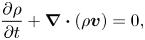 $$\begin{gather} \frac{\partial \rho}{\partial t}+\boldsymbol{\nabla} \boldsymbol{\cdot}(\rho \boldsymbol{v})=0 , \end{gather}$$
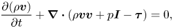 $$\begin{gather}\frac{\partial(\rho \boldsymbol{v})}{\partial t}+\boldsymbol{\nabla} \boldsymbol{\cdot}(\rho \boldsymbol{v} \boldsymbol{v}+p \boldsymbol{I}-\boldsymbol{\tau})=0, \end{gather}$$
 $$\begin{gather}\frac{\partial(\rho E)}{\partial t}+\boldsymbol{\nabla} \boldsymbol{\cdot}((\rho E+p) \boldsymbol{v}-\boldsymbol{\tau} \boldsymbol{\cdot} \boldsymbol{v}-\boldsymbol{q})=0 , \end{gather}$$
where  $\rho$, $\boldsymbol {v}$ and $p$ are density, velocity vector and pressure, respectively. Here, $E=p/[\rho (\gamma -1)]+\boldsymbol {v}\boldsymbol {\cdot }\boldsymbol {v}/2$ denotes the total energy, and $\boldsymbol {I}$ is the identity matrix. The viscous stress $\boldsymbol {\tau }$ and heat flux vector $\boldsymbol {q}$ are expressed according to
 $$\begin{gather}
\boldsymbol{\tau}=\frac{\mu\,Ma_{\infty}}{Re} \left(
\boldsymbol{\nabla}{\boldsymbol {v}} +
\boldsymbol{\nabla}{\boldsymbol{v}}^{{\rm T}}
-\frac{2}{3}\,(\boldsymbol{\nabla}\boldsymbol{\cdot}
\boldsymbol{v})\boldsymbol{I} \right),
\end{gather}$$
$$\begin{gather}
\boldsymbol{\tau}=\frac{\mu\,Ma_{\infty}}{Re} \left(
\boldsymbol{\nabla}{\boldsymbol {v}} +
\boldsymbol{\nabla}{\boldsymbol{v}}^{{\rm T}}
-\frac{2}{3}\,(\boldsymbol{\nabla}\boldsymbol{\cdot}
\boldsymbol{v})\boldsymbol{I} \right),
\end{gather}$$ $$\begin{gather}\boldsymbol{q}
=\frac{\mu\,Ma_{\infty}}{(\gamma-1)\, Pr \,
Re}\,\boldsymbol{\nabla} T,
\end{gather}$$
$$\begin{gather}\boldsymbol{q}
=\frac{\mu\,Ma_{\infty}}{(\gamma-1)\, Pr \,
Re}\,\boldsymbol{\nabla} T,
\end{gather}$$
where  $Ma_{\infty }$ is the Mach number, defined as $Ma_{\infty }=u_{\infty }/a_{\infty }$, and $u_{\infty }$ and $a_{\infty }$ are the free-stream velocity and sound speed, respectively. The free-stream quantities are denoted by subscript $\infty$. The Reynolds number $Re$ is defined as $Re=\rho ^*_{\infty } u^*_{\infty } l^*_{ref}/\mu ^*_{\infty }$, in which $l^*_{ref}$ is the reference length. The superscript $*$ denotes dimensional variables. The Prandtl number $Pr$ is set to 0.72. The dynamic molecular viscosity $\mu$ is approximated by Sutherland's law:
 \begin{equation} \mu (T) = {T}^{3/2}\,\frac{T_s^*/T^*_{\infty} + 1}{T^*_s/T^*_{\infty}+T}, \end{equation}
where  $T_{s}^*=110.4$ K. Here, $\rho _{\infty }^*$, $c_{\infty }^*$, $\rho _{\infty }^*c_{\infty }^{*2}$ and $T_{\infty }^*$ are employed in sequence to non-dimensionalise the density, velocity, pressure and temperature, respectively.
The in-house high-order finite-difference Navier–Stokes solver HiResX is used to solve the discretised governing equations, which has been well validated in previous studies (Ye et al. Reference Ye, Zhang, Wan, Sun and Lu2020; Zhuang et al. Reference Zhuang, Wan, Ye, Luo, Liu, Sun and Lu2023). To ensure numerical stability, a robust shock-capture scheme, the fifth-order AF-WENO, is utilised to treat the inviscid fluxes, and a sixth-order central difference scheme is used to discretise the viscous fluxes. For time advancement, the three-stage total variation diminishing Runge–Kutta method is utilised.
2.2. Resolvent analysis
We employ resolvent analysis to determine the most unstable disturbance characteristics of the mean flow with/without control. The concept and calculation of the resolvent can be found in Poulain et al. (Reference Poulain, Content, Sipp, Rigas and Garnier2023a). Here, we provide a concise introduction to resolvent analysis.
By applying a forcing  $\boldsymbol {f}$, we have rewritten (2.1)–(2.3) to obtain the form
 \begin{equation} \frac{\mathrm{d} \boldsymbol{q}}{\mathrm{d} t}=\boldsymbol{N}(\boldsymbol{q})+\boldsymbol{f}, \end{equation}
where  $\boldsymbol {q}=[\rho, \rho \boldsymbol {v}, \rho E ]^{\rm T}$, $\boldsymbol {N}$ is the discretised compressible Naiver–Stokes equation, and $\boldsymbol {f}$ represents the disturbances caused by the environment's noise, actuators, nonlinear interactions between disturbances, etc. Decompose $\boldsymbol {q}$ as $\boldsymbol {q} = \bar {\boldsymbol {q}} + \boldsymbol {q}'$, in which $\bar {\boldsymbol {q}}$ is base flow and $\boldsymbol {q}'$ is disturbance. Considering that the amplitudes of disturbance $\boldsymbol {q}'$ and forcing $\boldsymbol {f}$ are small, we then obtain
 \begin{equation} \frac{\mathrm{d} \boldsymbol{q}^{\prime}}{\mathrm{d} t}=\boldsymbol{A} \boldsymbol{q}^{\prime}+ \boldsymbol{f}. \end{equation}
 The Jacobian matrix  $\boldsymbol {A}$ is obtained as $\boldsymbol {A}=\mathrm {d} \boldsymbol {N} /\mathrm {d} \boldsymbol {q}|_{\bar {q}}$. We suppose that the harmonic forcing with a spatial structure is $\boldsymbol {f}(x, y, t)=\tilde {\boldsymbol {f}}(x, y)\, \mathrm {e}^{\mathrm {i} \omega t}$, and its response with the form $\boldsymbol {q}^{\prime }(x, y, t)=\tilde {\boldsymbol {q}}(x, y)\, \mathrm {e}^{\mathrm {i} \omega t}$ is established as
 \begin{equation} \tilde{\boldsymbol{q}}=\boldsymbol{R}\tilde{\boldsymbol{f}}, \end{equation}
where  $\boldsymbol {R}=(\mathrm {i} \omega \boldsymbol {I}-\boldsymbol {A})^{-1}$ is the resolvent operator, and $\omega$ is the angular frequency.
To evaluate the energy of  $\tilde {q}$, the definition in Chu (Reference Chu1965) and George & Sujith (Reference George and Sujith2011) is used, which is written as
 \begin{equation} E_{Chu}=\|\tilde{\boldsymbol{q}}\|_E^2= \frac{1}{2} \int_{\varOmega} \left( \bar{\rho}\, | \tilde{\boldsymbol{v}} |^2 + \frac{ \bar{T} } { \gamma\,Ma_{\infty}^2\, \bar{\rho}}\,| \tilde{\rho}|^2 + \frac{ \bar{\rho} }{ (\gamma-1)\gamma\,Ma_{\infty}^2\, \bar{T} }\,|\tilde{T}|^2 \right) \mathrm{d} \varOmega, \end{equation}
where  $\varOmega$ is the integration domain. It is selected to be the whole computational domain in this study. The definition of $\|\tilde {\boldsymbol {q}}\|_E^2$ can also be written in the form $\|\tilde {\boldsymbol {q}}\|_E^2 =\tilde {\boldsymbol {q}}^{\mathrm {T}}\boldsymbol{\mathsf{Q}}_E\tilde {\boldsymbol {q}}$, in which $\boldsymbol{\mathsf{Q}}_E$ is a discrete Hermitian matrix. Superscript $\mathrm {T}$ means the transconjugate operator. It is commonly employed for investigating the global behaviour of compressible flows due to its inclusion of terms pertaining to both thermodynamic and kinetic disturbances. To evaluate the energy of $\tilde {\boldsymbol {f}}$, the discrete inner product is utilised:
 \begin{equation} \|\,\tilde{\boldsymbol{f}}\|_F^2=\int_{\varOmega} \bar{\rho}^{-1} {\tilde{\boldsymbol{f}}}^{\mathrm{T}} \tilde{\boldsymbol{f}} \,\mathrm{d} \varOmega . \end{equation}
The definition  $\|\tilde {\boldsymbol {f}}\|_F^2$ can be rewritten with a Hermitian matrix $\boldsymbol{\mathsf{Q}}_F$ as $\|\tilde {\boldsymbol {f}}\|_F^2 =\tilde {\boldsymbol {f}}^{\mathrm {T}}\boldsymbol{\mathsf{Q}}_F{\tilde {\boldsymbol {f}}}$. A prolongation/restriction matrix $\boldsymbol {P}$ is introduced to restrict the region of forcing in the flow or to specify the components. In this investigation, only the momentum components are chosen for the forcing field. Replacing $\tilde {\boldsymbol {f}}$ by $\boldsymbol {P}\tilde {\boldsymbol {f}}$, we can find a specific solution that has the maximum gain
 \begin{equation} \tilde{g}^2(\omega) =
\sup _{\tilde{\boldsymbol{f}} {\neq} 0}
\frac{\|\tilde{\boldsymbol{q}}\|_E^2}
{\|\,\tilde{\boldsymbol{f}}\|_F^2}
=\sup_{\tilde{\boldsymbol{f}} {\neq} 0}
\frac{\tilde{\boldsymbol{f}}^\mathrm{T}
\boldsymbol{P}^\mathrm{T} \boldsymbol{R}^\mathrm{T} \boldsymbol{\mathsf{Q}}_E
\boldsymbol{R}\boldsymbol{P}\tilde{\boldsymbol{f}}}
{\tilde{\boldsymbol{f}}^\mathrm{T} \boldsymbol{\mathsf{Q}}_F
\tilde{\boldsymbol{f}}}.
\end{equation}
\begin{equation} \tilde{g}^2(\omega) =
\sup _{\tilde{\boldsymbol{f}} {\neq} 0}
\frac{\|\tilde{\boldsymbol{q}}\|_E^2}
{\|\,\tilde{\boldsymbol{f}}\|_F^2}
=\sup_{\tilde{\boldsymbol{f}} {\neq} 0}
\frac{\tilde{\boldsymbol{f}}^\mathrm{T}
\boldsymbol{P}^\mathrm{T} \boldsymbol{R}^\mathrm{T} \boldsymbol{\mathsf{Q}}_E
\boldsymbol{R}\boldsymbol{P}\tilde{\boldsymbol{f}}}
{\tilde{\boldsymbol{f}}^\mathrm{T} \boldsymbol{\mathsf{Q}}_F
\tilde{\boldsymbol{f}}}.
\end{equation} The corresponding  $\tilde {\boldsymbol {f}}$ and $\tilde {\boldsymbol {q}}$ are called optimal forcing and response mode, respectively. The optimisation problem can be converted into the generalised Hermitian eigenvalue problem:
 \begin{equation}
\boldsymbol{P}^{\rm T}
\boldsymbol{R}^{\rm T} {\boldsymbol{\mathsf{Q}}}_E
\boldsymbol{R} \boldsymbol{P} \tilde{\boldsymbol{f}}=\mu^2
{\boldsymbol{\mathsf{Q}}}_F \tilde{\boldsymbol{f}}.
\end{equation}
\begin{equation}
\boldsymbol{P}^{\rm T}
\boldsymbol{R}^{\rm T} {\boldsymbol{\mathsf{Q}}}_E
\boldsymbol{R} \boldsymbol{P} \tilde{\boldsymbol{f}}=\mu^2
{\boldsymbol{\mathsf{Q}}}_F \tilde{\boldsymbol{f}}.
\end{equation} To obtain the optimal gain, it is necessary to compute the largest eigenvalue of the positive generalised eigenvalue problem. The calculations of resolvent analysis are performed with the solver BROADCAST (Poulain et al. Reference Poulain, Content, Sipp, Rigas and Garnier2023a). To calculate the Jacobian matrix  $\boldsymbol {A}$, a high-order FE-MUSCL (flux-extrapolated-MUSCL) scheme is used to discretise the convective flux, and a five-point compact scheme to discretise the viscous flux.
2.3. The DNS set-up
A Mach number 5.86 plate boundary layer is used to investigate the control effect on the instability of steady blowing/suction. The free-stream temperature is  $T^*_{\infty } = 55$ K, density is $\rho ^*_{\infty }=0.0443\ {\rm kg}\ {\rm m}^{-3}$, and velocity is $U^*_\infty = 870\ {\rm m}\ {\rm s}^{-1}$, which are the same as in a previous investigation (Zhang, Duan & Choudhari Reference Zhang, Duan and Choudhari2017). A sketch of the computational domain is shown in figure 1, and the reference length $l_{ref}^*$ satisfies $Re=\rho ^*_\infty U^*_\infty l_{ref}^*/\mu _\infty ^*=38\,300$. The inflow boundary starts at $x_0=0$, with its distance $d_0^*$ to the leading edge satisfying $Re_0=\sqrt {Re_{d0}} =\sqrt {\rho ^*_\infty U_\infty ^* d_0^*/\mu _\infty ^*} = 1000$. The computational domain length in the streamwise direction is $L^*$, satisfying $Re_{L}=\sqrt {\rho ^*_\infty U_\infty ^* (d_0^*+L^*)/\mu _\infty ^* }=4500$. The length in the wall-normal direction is $50l_{ref}^*$; 5120 grid points are used in the streamwise direction, while 300 grid points are clustered near the wall in the wall-normal direction.
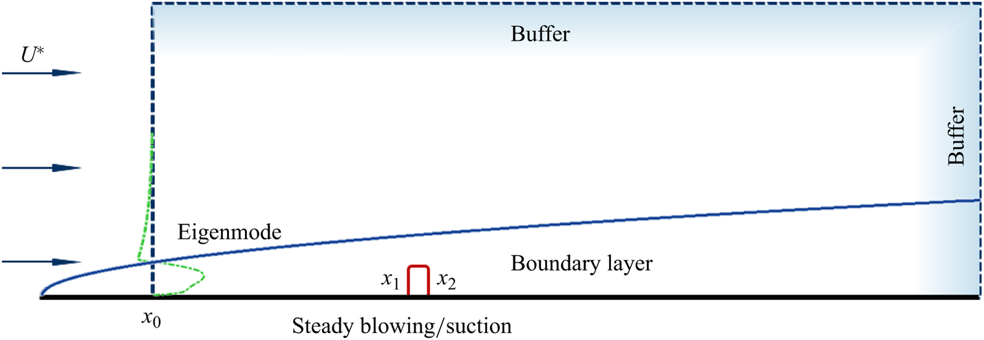
Figure 1. Sketch of the DNS domain over a flat plate, along with the boundary conditions.
The inlet disturbances are introduced as eigenmodes obtained from spatial linear stability theory (Malik Reference Malik1990). To ensure that the disturbance evolves linearly, its amplitude is set to be of the order of  $10^{-5}$. Free-stream conditions are imposed at the outer and downstream regions of the boundary layer, while adiabatic and no-slip boundary conditions are applied at the wall. Buffer zones are employed upstream and downstream of the boundary layer to mitigate disturbances.
The blowing/suction slot is located at  $[x_1,x_2]$, where $x_1$ is fixed at 89.9, and $x_2=x_1+d$, with $d$ representing the slot width. The control of blowing/suction is represented by the model
 \begin{equation} v(x,t) = \left\{ \begin{array}{@{}ll} A_c, & x\in[x_1,x_2], \\[2pt] 0, & x\notin[x_1,x_2]. \end{array} \right. \end{equation}
 The density in the slot remains constant at  $\rho _{wall}=0.152$. For convenience, the flux of control can be defined as $\mathcal {F}_c=A_cd$. The control parameters are summarised in table 1. In each case, eleven uniformly spaced frequency disturbances between $F=4.5\times 10^{-5}$ and $F=7.5\times 10^{-5}$ are employed, where $F=2{\rm \pi} f^*/(\rho _\infty ^* U_\infty ^{*2})$, in which $f^*$ denotes dimensional frequency. These frequencies are chosen to be around the synchronisation frequency. In the DNS investigation, the spanwise wavenumber $\beta$ of disturbance is selected as 0, $4.5\times 10^{-5}\ (\beta _1)$ and $9\times 10^{-5}\ (\beta _2)$ for each frequency, in which the reference length used to define $\beta$ is $\mu _\infty ^*/(\rho _\infty ^* U_\infty ^*)$. Each spanwise wavelength is resolved by 30 grid points when the spanwise wavenumber is not zero. For cases with slot width 1, approximately 20 grid points are used to resolve the slot. Additionally, it is noteworthy that the implementation of such control measures in practical applications may also be anticipated in future, according to some previous experiment investigations (Miró Miró et al. Reference Miró Miró, Dehairs, Pinna, Gkolia, Masutti, Regert and Chazot2019; Prokein & von Wolfersdorf Reference Prokein and von Wolfersdorf2019).
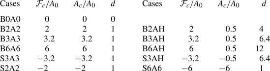
Table 1. Simulation parameters for various cases.  $A_0$ is $0.01U_\infty ^*$. The B or S in the notation indicates the flux of blowing or suction control and A indicates the amplitude.
3. Mean flow modified by blowing or suction
The linear evolution of the flow downstream is determined by the characteristics of the new base flow for the small-amplitude disturbances of the incoming flow that we investigate. As a result, the initial depiction focuses on the characteristic changes in the mean flow.
Figure 2 depicts the near-wall pressure evolution for all cases. It is seen that the pressure gradually rises upstream of the blowing slot, resulting in an adverse pressure gradient for each blowing case. Meanwhile, within the blowing slot interval, the pressure returns to the downstream amplitude, resulting in a zone of favourable pressure gradient. Hence for a narrower blowing slot, such as case B2A2 illustrated in figure 2(a), it induces a rapid pressure drop, whereas for wider slots, as in case B2AH shown in figure 2(b), the length of the favourable pressure gradient zone would be extended to approximately 4. The pressure peak increases correspondingly with an increased blowing amplitude under the same blowing flux. The suction creates two regions characterised by a favourable pressure gradient and an adverse pressure gradient, respectively, which is in direct contrast to the blowing. Furthermore, it should be emphasised that the zone of adverse pressure gradient extends beyond the leading edge of the suction and encompasses the entire suction slot.
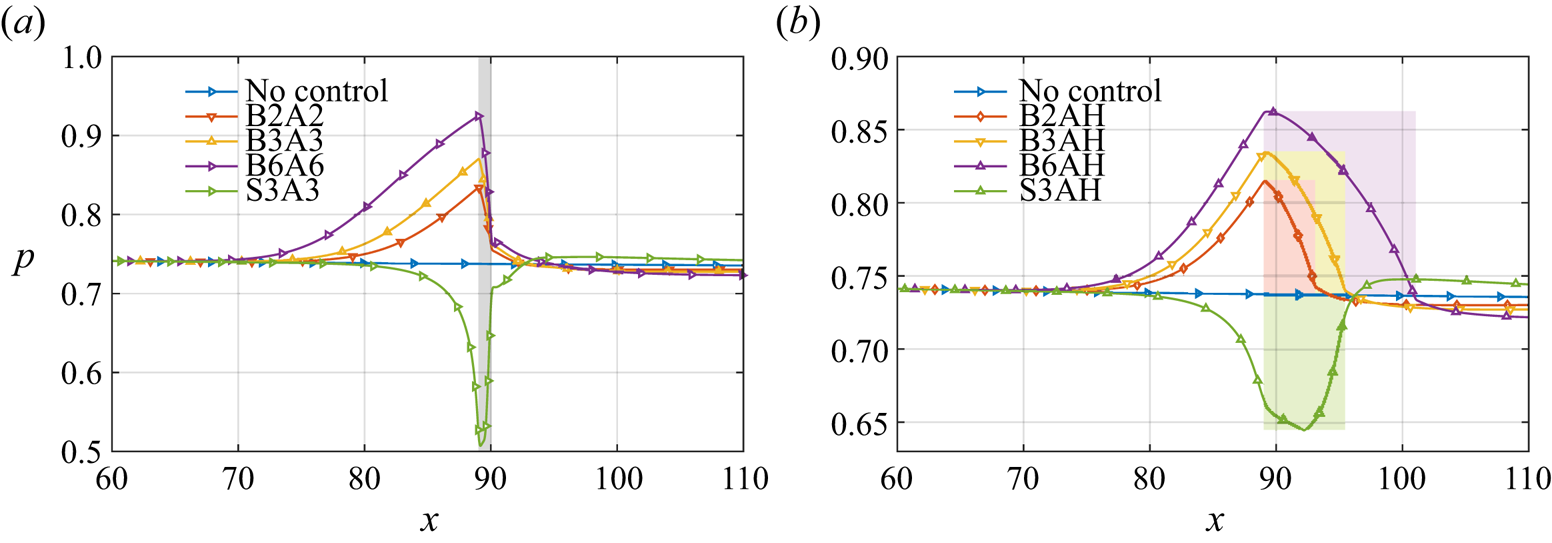
Figure 2. The streamwise evolution of pressure near the wall in cases (a) B2A2, B3A3, B6A6, S3A3, and (b) B2AH, B3AH, B6AH, S3AH. The grey rectangular background represents the streamwise range of the blowing/suction in (a). The purple, yellow, red and green rectangular backgrounds represent the streamwise ranges of slots for cases B2AH, B3AH, B6AH and S3AH, respectively.
As shown in figure 3, the waveguide, which consists of the wall surface and the sonic line, becomes wider and then narrows slightly near the blowing; it undergoes an opposite trend near the suction region. Previous studies (Mack Reference Mack1990; Fedorov Reference Fedorov2011) have suggested that the second mode can be interpreted as acoustic rays reflecting between the sonic line and wall surface. Hence an analysis of variations in the sonic line is conducted to describe qualitatively how boundary layer thickness or thinness induced by blowing or suction influences disturbance development. Currently, the phase speed chosen to extract the sonic line is 5.5, which corresponds to the phase speed (using  $c$ at $x\approx 90$) of a perturbation whose synchronisation point is located at the control position. The sonic line rises/falls rapidly upstream during blowing/suction, then falls/rises to a height above/below the uncontrolled height downstream. It is evident that a strong non-parallel effect occurs, and its impact on the growth of disturbances will be analysed in § 5. Here, we focus on the influence on the disturbance phase speed.
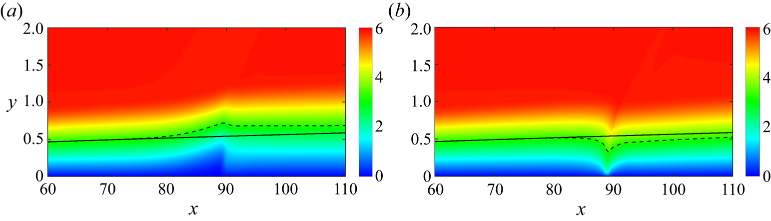
Figure 3. The streamwise velocity contours in (a) case B3A3 and (b) case S3A3. The black line is the sonic line ( $c=U+a$) whose phase speed is $c=5.5$ without control (solid line) and with control (dashed line).
The phase speed of the perturbed wave is analysed to investigate the variation in the near-wall pressure disturbance using the fast Fourier transform (FFT) and synchrosqueezed wavelet analysis (Daubechies, Lu & Wu Reference Daubechies, Lu and Wu2011). The FFT is used to obtain the specific frequency response. The synchrosqueezed wavelet transform is an effective signal-processing technique that combines wavelet analysis with a process called synchrosqueezing. By combining these two techniques, synchrosqueezed wavelet analysis provides a powerful tool for analysing signals with time-varying frequency content, such as non-stationary signals encountered in many real-world applications. Presently, this method is employed mainly to ‘sharpen’ the space–wavenumber representation compared with conventional wavelet analysis. The Bump wavelet is employed to analyse the instantaneous pressure at the line  $y=0.1$ between $x\approx 10$ and $x=200$ for two typical cases, i.e. B3A3 and S3A3. The results near the blowing or suction are shown in figure 4. For a low-frequency disturbance with $F=4.8\times 10^{-5}$ in case B3A3, the wavenumber of the disturbance increases gradually upstream of the blowing, resulting in a decrease in the phase speed. However, the wavenumber decreases gradually near the blowing. The change in wavenumber and the change in height of the sonic line follow essentially the same trend. As shown in figure 4(b), for a high-frequency disturbance with $F=7.2\times 10^{-5}$, there is also a tendency for the phase speed to decrease upstream of the blowing, while a relatively new disturbance with a higher wavenumber appears downstream. Then the new disturbance decays, and the predominant disturbance becomes the second mode downstream. The opposite result for suction can be observed in figures 4(c,d), where for high frequencies, the phase speed of the disturbance decays more significantly. This may be related to the different wavelengths of the disturbances, as longer waves are more susceptible to changes in their phase speed. Moreover, as shown in figure 4(d), it is also found that the disturbance with $F=7.2\times 10^{-5}$ is enhanced more significantly by suction control; the underlying mechanism of this enhancement is attributed mainly to the reduced boundary layer thickness, which will be analysed further in the following. In summary, it can be concluded that there is a tendency for the phase speed of the perturbed wave to decrease as the height of the sonic line increases, and vice versa, with the degree of change being frequency-dependent.
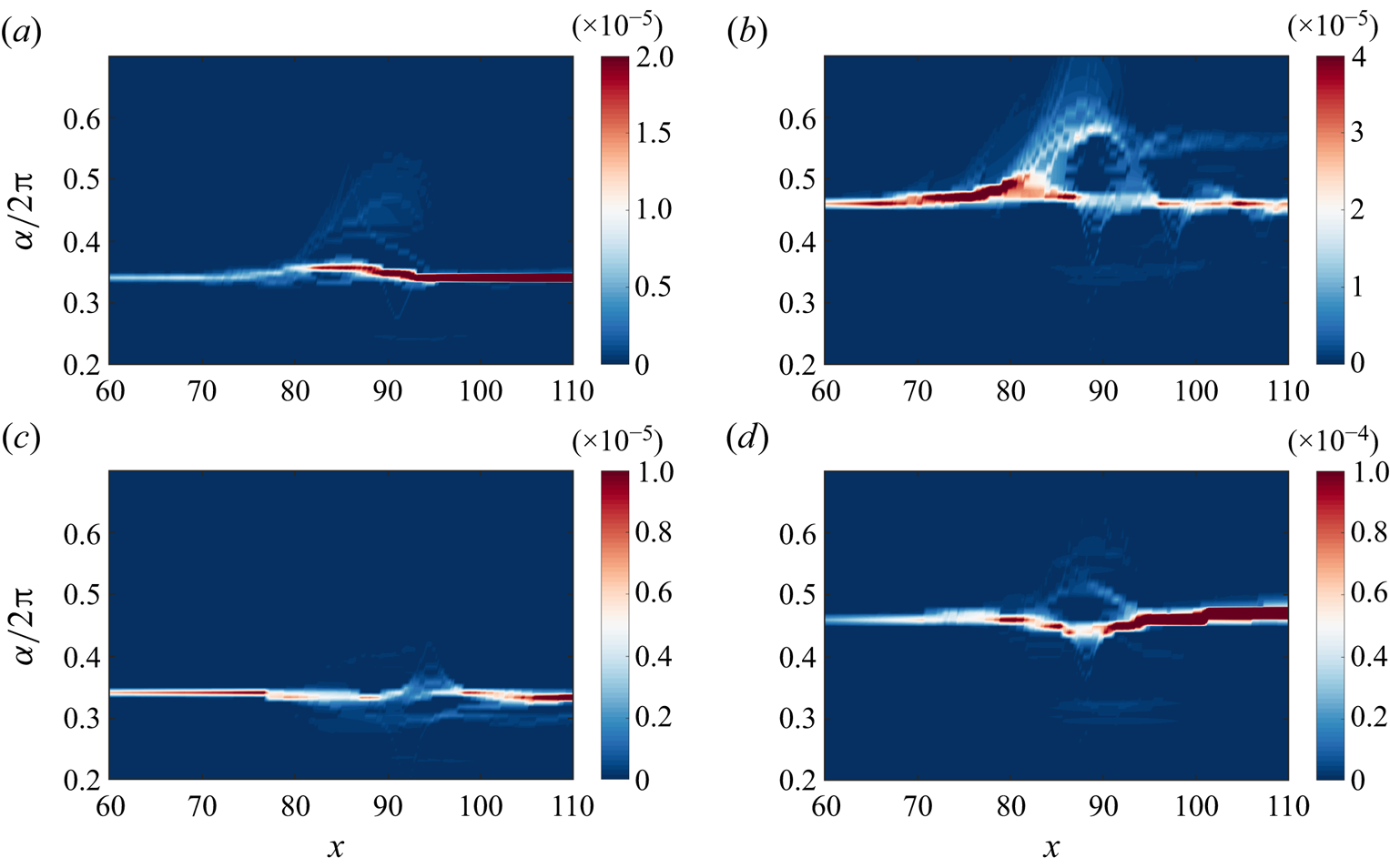
Figure 4. The wavenumber evolution obtained by the wavelet analysis operated on the pressure near the wall: (a)  $F=4.8\times 10^{-5}$ in case B3A3, (b) $F=7.2\times 10^{-5}$ in case B3A3, (c) $F=4.8\times 10^{-5}$ in case S3A3, (d) $F=7.2\times 10^{-5}$ in case S3A3.
4. The control effect of blowing/suction flux and amplitude
This section presents the control effect of blowing/suction on disturbances of different frequencies and then analyses the influence of blowing/suction flux and amplitude on the control effect, which is based on DNS and resolvent analysis, respectively. The DNS analyse the spatial growth of local eigenmodes at each streamwise station since disturbance is added from the inlet in the form of eigenmodes obtained from local spatial stability analysis. If the base flow does not change drastically in the streamwise direction with control, then DNS can be replaced by tools such as linear spatial stability analysis, as demonstrated in previous studies (Fedorov et al. Reference Fedorov, Soudakov, Egorov, Sidorenko, Gromyko, Bountin, Polivanov and Maslov2015; Dong & Zhao Reference Dong and Zhao2021). In contrast to DNS, resolvent analysis focuses on the global eigenmodes of a specific zone, which can be regarded as the dominant amplification mode for spatially distributed disturbances at a given frequency in terms of sensitivity. For hypersonic boundary layers, resolvent analysis can also yield Mack first/second modes that are essentially equivalent to those obtained through local stability analysis, as described in Nibourel et al. (Reference Nibourel, Leclercq, Demourant, Garnier and Sipp2023).
4.1. Control effect on the mode amplitude
Before discussing the control effect of blowing and suction, it is crucial to define the amplification coefficient ( $C_A$) to evaluate its effectiveness. In this study, the amplification coefficient is defined as the ratio between the maximum values of $|u'|$ obtained with and without blowing/suction in a sufficiently long computational domain that allows reaching the disturbance's maximum value. Figure 5 presents the streamwise evolution of mode amplitude without and with blowing or suction. We find that the control effects are frequency-dependent. For instance, the disturbance with frequency $F=4.8\times 10^{-5}$ is amplified, reaching amplification coefficient 1.38 by comparing case B6A6 with case B0A0. However, for frequency $F=5.1\times 10^{-5}$, the disturbance is damped and reaches a corresponding coefficient 0.40 by comparing case S3A3 with case B0A0. Meanwhile, it is noted that the evolution of the disturbance near the blowing has a strong influence on the amplification factor. For example, as shown in figure 5(b), for case B6A6, the disturbance amplitude drops from $0.6\times 10^{-3}$ to $0.2\times 10^{-3}$ approximately in the range $x\in [89,95]$. The dramatic changes in the vicinity of blowing or suction will decrease the overall amplification factor.
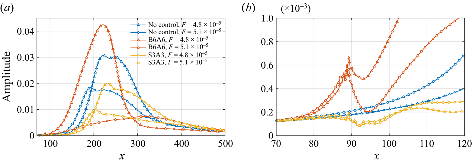
Figure 5. The streamwise evolution of mode amplitude for defining the amplification coefficient (a) in a relatively long distance, (b) near the blowing/suction.
Figure 6 presents the amplification coefficients for different disturbance frequencies in control cases. The most dangerous 2-D instability is examined first. It is important to note that there exists a critical frequency for blowing control, beyond which the disturbance is suppressed within a specific frequency range, while below this frequency, it continues to amplify. For instance, in case B2A2, the critical frequency is approximately  $F=5.4\times 10^{-5}$, as shown in figure 6(a). When the disturbance has a frequency greater than $F=7.2\times 10^{-5}$, its amplification coefficient reaches 1 since the location where the mode reaches its maximum amplitude is far upstream of the blowing. Within the suppression band, there exists a minimum amplification coefficient 0.3 at frequency approximately $F=6\times 10^{-5}$ in case B2A2. Additionally, among the calculated frequencies, there also exists a maximum value within an amplification band with maximum amplification coefficient 4 at approximately $F=4.8\times 10^{-5}$. Figures 6(a)–6(c) all show that there is a slight discrepancy in the amplification coefficients for cases with slot width 1 and control amplitude 0.5. This implies that the influence of blowing amplitudes on the control effect, including critical frequency and minimum amplification coefficient, is relatively insignificant when considering the same blowing flux.

Figure 6. The dependency of amplification coefficient  $C_A$ on the frequencies for different fluxes. Blowing control with the flux of (a) $\mathcal {F}_c=2$, (b) $\mathcal {F}_c=3.2$ and (c) $\mathcal {F}_c=6$. Suction control with the flux of (d) $\mathcal {F}_c=-3.2$. The blue vertical dashed line is the synchronisation frequency.
Previous studies (Duan et al. Reference Duan, Wang and Zhong2013; Zhao et al. Reference Zhao, Dong and Yang2019a) have suggested that the synchronisation frequency may act as the critical frequency. Therefore, in figure 6, we mark the synchronisation frequency. When the control flux is relatively small, such as in case B2A2, the critical frequency is close to the synchronisation frequency. However, as the blowing flux increases, the critical frequency rapidly shifts to lower frequencies and widens the suppression frequency band. As the flow flux increases from 2 to 6, the critical frequency decreases from approximately  $5.4\times 10^{-5}$ to $4.8\times 10^{-5}$. The increase in flux also improves the suppression effect, resulting in a decrease in the minimum amplification factor from 0.3 to 0.13. However, for all cases of increased flux levels, there are only slight changes around 6 for the corresponding frequencies of minimum amplification factors, indicating that relatively small changes occur at these frequencies. Additionally, with an increase in blowing flux level, there is a slight increase in discrepancy between amplification coefficients of different amplitudes at the same flux levels, suggesting that local base flow changes due to blowing or suction have a greater impact on mode growth rate. Figure 6(d) illustrates the suppression effect of suction control, which also has a critical frequency (approximately $F=6.1\times 10^{-5}$ in this case). Unlike blowing control, suction control suppresses disturbances below the critical frequency while promoting higher-frequency disturbances. Additionally, for the disturbances studied here with frequency band $4.5\times 10^{-5}< F<6\times 10^{-5}$, the suction cases all show similar suppression effects. Disturbances with higher frequencies are promoted, which is also observed in figure 4(d). The maximum promoted effect is achieved around the frequency of $6.9\times 10^{-5}$ approximately. When the suction flux is constant, the influence of suction amplitude on the control effect of disturbances with frequencies less than or equal to $6.0\times 10^{-5}$ is nearly negligible.
Next, we shift our focus to the control effects on the oblique waves. In general, the suppression/promotion effect of blowing on the lower spanwise wavenumber ( $\beta _1$) instability is essentially similar to the results of the control effect on the 2-D instability, i.e. suppressing the high-frequency disturbances while promoting lower-frequency disturbances, as shown in figure 6. However, for the $\beta _1$ disturbances, the critical frequency is shifted to a higher value, resulting in a narrow suppression frequency band. Meanwhile, the overall promotion or suppression effects become weaker compared with the control on the 2-D disturbances, and the frequencies corresponding to the maximum promotion and suppression effects are shifted to higher values. For instance, for 2-D mode, the maximum promotion effect is obtained at $F\approx 4.8\times 10^{-5}$, while this frequency moves to $F=5.4\times 10^{-5}$ for the $\beta _1$ disturbance. The increase in blowing flux leads to a corresponding shift of the critical frequency towards lower values, resulting in a wider suppression bandwidth. The maximum promotion or suppression effects become stronger. Additionally, compared to the control on 2-D disturbances, for suction control, the critical frequency increases and its suppression bandwidth widens within the studied parameter range. The amplification factor remains similar in the low-frequency band $4.5\times 10^{-5}< F<6.0\times 10^{-5}$, while in the high-frequency band, the amplification effect weakens. The impact of amplitude variation on the mode suppression effect is less significant compared to the control flux. For a disturbance with a higher spanwise wavenumber ( $\beta _2$), the critical frequency continues to shift towards higher frequencies, and the overall suppression effects become much weaker and even disappear within the investigated frequency range. In B2A2, it is seen that the suppression effect exists only in the high-frequency band ( $F>7.2\times 10^{-5}$), and the lower-frequency disturbances are weakly promoted. As the control amplitude increases, the promoting effect is slightly enhanced, while the critical frequency moves towards a higher value. In B6A6, the suppression effect disappears within the investigated frequency range. As control flux increases, the peak frequency of the promotion effects is reduced, shifting from $F=6.6\times 10^{-5}$ at B2A2 to $6.0\times 10^{-5}$ at B6A6, and the trend is the same as that of suppression. Similarly, the control on higher spanwise wavenumber disturbances under suction control exhibits a weaker suppression effect in the frequency band.
4.2. Control effect on the optimal disturbance
In this subsection, we evaluate the control effect by comparing the gain of optimal disturbance obtained with and without blowing or suction. A larger gain indicates that input at the same energy norm induces a response with higher global energy, i.e. a larger mode growth. The computational domain used for resolvent analysis is  $[0,200]$, discretised with 1000 uniform grid points. The normal computational domain is $[0,5]$, and the normal grid consists of 150 points, distributed in the same manner as in previous studies (Poulain et al. Reference Poulain, Content, Sipp, Rigas and Garnier2023a), clustering near the wall. We choose $x=200$ as the end of the current computational domain, which is far downstream from the blowing and suction. It should be noted that the streamwise size of the computational domain generally affects gain calculation, but it is sufficient for our purpose of analysing control effects. For the disturbance with frequency $F=6.0\times 10^{-5}$, there are 14 grid points per wavelength, approximately. This resolution has been shown to be sufficient in previous studies (Poulain et al. Reference Poulain, Content, Sipp, Rigas and Garnier2023a) (12 grid points per wavelength). The base flow used for resolvent analysis is obtained through DNS.
Figure 7 shows the optimal gain given by resolvent analysis in uncontrolled case B0A0 within the parameter space of frequency and spanwise wavenumber  $(F,\beta )$. Two peak regions can be observed from the background and are the $F\unicode{x2013}\beta$ range important for transition control. Those two peak regions of optimal gain are consistent with previous investigations (Guo, Hao & Wen Reference Guo, Hao and Wen2023; Poulain et al. Reference Poulain, Content, Rigas, Garnier and Sipp2024). To measure the control effect, we define a ratio $\mu _c/\mu _{uc}$, where $\mu _c$ denotes the optimal gain with control, and $\mu _{uc}$ denotes the optimal gain without control. Figure 8 illustrates the contours of $\mu _c/\mu _{uc}$ in controlled cases, where the curve of $\mu _c/\mu _{uc}=1$ in the high optimal region is defined as the critical curve. In blowing control cases, the 2-D disturbances ( $\beta =0$) with lower frequencies are generally promoted ( $\mu _c/\mu _{uc}>1$), while those with higher frequencies are damped ( $\mu _c/\mu _{uc}<1$). In figure 8(a), the critical frequency is approximately $F=5.6\times 10^{-5}$ with $\beta =0$ in case B2A2. With an increased $\beta$, the critical frequency of the three-dimensional disturbance tends to shift towards a higher frequency. As the control amplitude increases from $2A_0$ to $6A_0$, the critical frequency for 2-D disturbances decreases from $F=5.6\times 10^{-5}$ to $F=5.0\times 10^{-5}$, approximately, the suppression effect is enhanced, and the critical curve moves towards the lower frequency direction, as shown in figures 8(a–c). This trend is also summarised clearly in figure 7. When comparing figure 8(c) with figure 8(a), it is further found that the maximum value of $\mu _c/\mu _{uc}$ is enhanced. The critical curve form for suction control resembles that of blowing control; however, suction mainly suppresses low-frequency disturbances while promoting high-frequency ones, as depicted in figures 8(d–f). With increased suction amplitude, the critical curve shifts towards a higher frequency direction, as illustrated in figure 7.
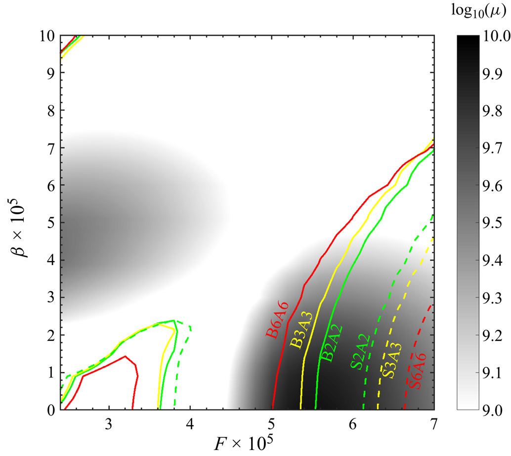
Figure 7. The grey background shows the optimal gain distribution with respect to  $F$ and $\beta$ for the uncontrolled case B0A0. The solid/dashed lines denote contours of $\mu _c/\mu _{uc}=1$, in which $\mu _c$ is the optimal gain in controlled cases, and $\mu _{uc}$ is the optimal gain in uncontrolled case B0A0. Those curves that follow in the high optimal gain region are critical curves.
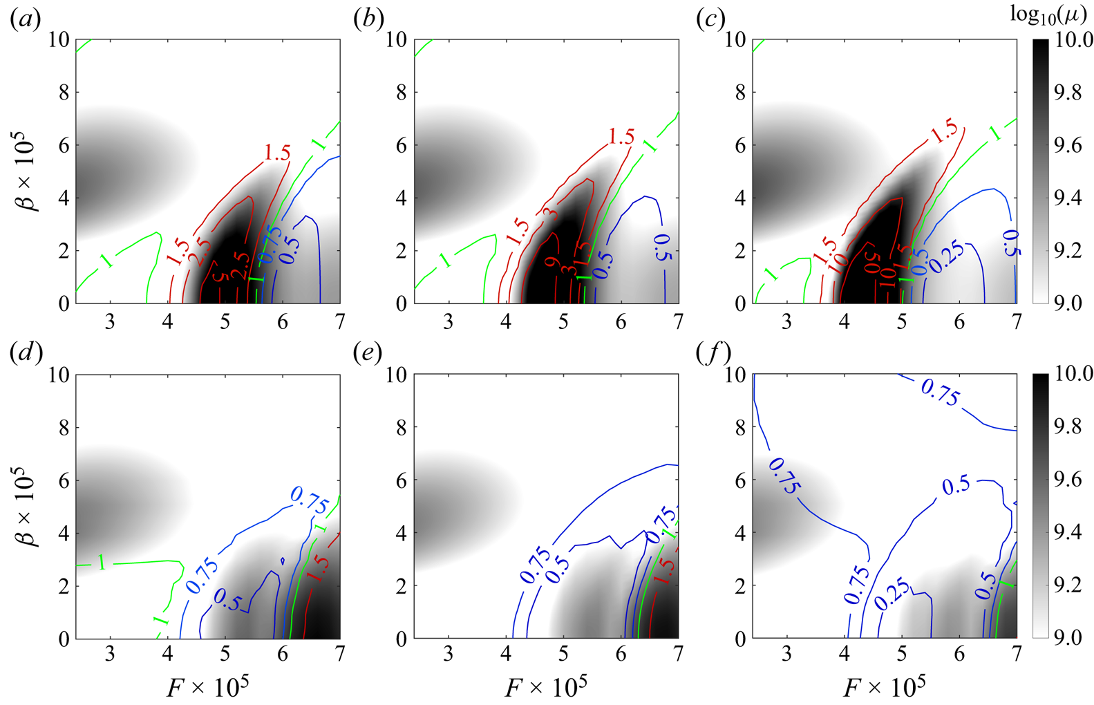
Figure 8. The grey background shows the optimal gain with respect to  $F$ and $\beta$ for controlled cases: (a) B2A2, (b) B3A3, (c) B6A6, (d) S2A2, (e) S3A3, (f) S6A6. The solid lines denote contours of different $\mu _c/\mu _{uc}$, in which $\mu _c$ is the optimal gain in controlled cases, and $\mu _{uc}$ is the optimal gain in case B0A0.
Figure 9 compares contours with the same blowing flux but different blowing amplitudes, and it is demonstrated that the effect of blowing control amplitude on the optimal gain distribution concerning  $F$ and $\beta$ is relatively weak. For a small blowing flux, the contours align closely; however, for higher blowing amplitudes, they exhibit slight discrepancies primarily in areas corresponding to relatively high optimal gain. Additionally, suction results were analysed (see figure 9d) and found to show relatively consistent contours, albeit with some deviations in regions of high gain. In short, the major findings of resolvent analysis for blowing/suction control are generally consistent with those obtained from DNS, including variations in the critical frequency as the blowing flux changes and the maximum suppression effect is achieved at different blowing fluxes. Additionally, we note that varying the blowing/suction amplitude at a constant control flux yields minor effects on the control outcomes.
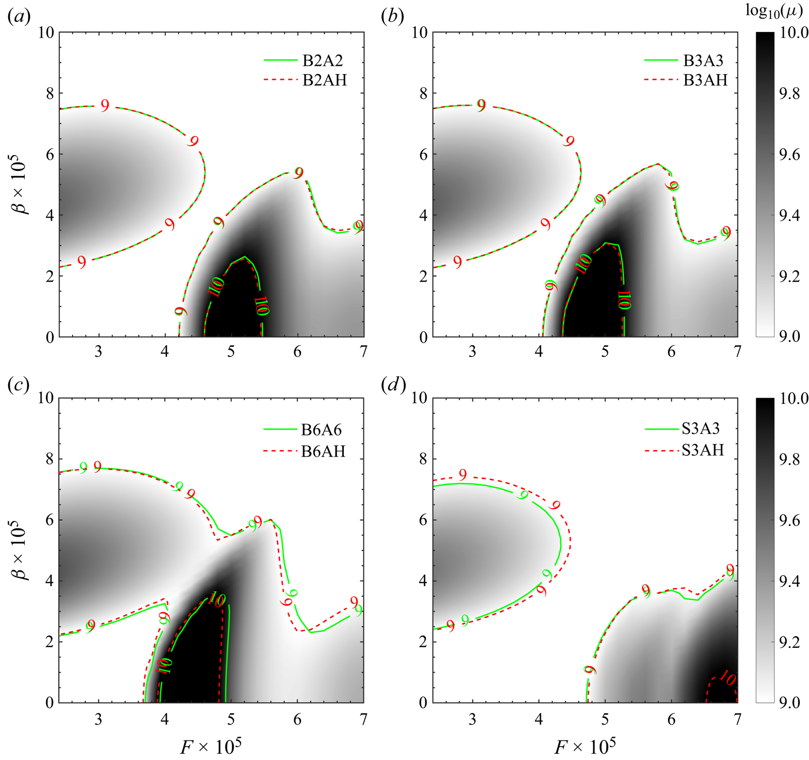
Figure 9. Comparison of optimal gains with the same control flux but different control amplitude. The grey background shows optimal gain with respect to  $F$ and $\beta$ for controlled cases: (a) B2A2, (b) B3A3, (c) B6A6, (d) S3A3. Solid lines denote those contours of $\log _{10}(\mu )$ in cases B2A2, B3A3, B6A6 and S3A3, respectively. Dashed lines denote those contours of $\log _{10}(\mu )$ in cases B2AH, B3AH, B6AH and S3AH, respectively.
The forcing and response modes were examined in figure 10 to better understand the changes in the optimal forcing and response modes under control for disturbances with  $F = 4.5\times 10^{-5}$ in cases B3A3 and S3A3, under which condition disturbances are all suppressed. Previous results of the hypersonic boundary layer without control (Nibourel et al. Reference Nibourel, Leclercq, Demourant, Garnier and Sipp2023; Poulain et al. Reference Poulain, Content, Sipp, Rigas and Garnier2023a) show that the forcing modes are distributed primarily around the generalised inflection point (GIP), with amplification mechanisms related to the convective-type non-normality and component-type non-normality (Orr mechanism) (Bugeat et al. Reference Bugeat, Chassaing, Robinet and Sagaut2019; Nibourel et al. Reference Nibourel, Leclercq, Demourant, Garnier and Sipp2023). In the case of blow control, the forcing modes remain predominantly distributed around the GIP, although blowing causes a local upward bias of the GIP, and the inclined pattern also suggests that there is no change in the amplification mechanism. Two new features emerge in the response mode: first, an outward radiating component is present in proximity to blowing; second, there is a rapid decrease in amplitude as disturbance crosses through the control jet, which aligns with suppression observed in DNS (see figure 5). The forcing modes of suction control are distributed mainly near the GIP, resulting in a local downward bias of the GIP. Additionally, there is a new sensitive region near suction at $x=90$, possibly due to an increased local shear rate caused by suction. However, its corresponding mode only exhibits thinning of the boundary layer downstream of suction.
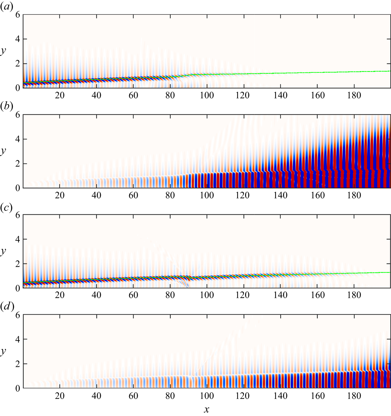
Figure 10. The (a,c) forcing and (b,d) response modes in cases (a,b) B3A3 and (c,d) S3A3, with  $F=4.5\times 10^{-5}$. The green dashed line is the GIP near the boundary edge.
5. The control mechanisms
In the previous section, it was found that disturbances with a higher frequency are dampened for blowing control, while disturbances with a lower frequency are dampened for suction control. In this section, we aim to reveal the control mechanisms behind mode suppression. Far away from the blowing or suction, the growth rate of disturbances is determined mainly by stability characteristics. The base flow can be seen as a thickened or thinned boundary layer, which supports the idea that when the boundary layer becomes thicker/thinner, the critical frequency becomes lower/higher because the new base flow synchronisation frequency tends to become lower/higher. Moreover, high-frequency disturbances tend to be suppressed due to a shorter instability range when the boundary thickens. However, near the blowing/suction, the thickness of the base flow varies rapidly, with a noticeable adverse/favourable pressure gradient and a compression/rarefaction wave. These changes significantly impact the overall amplification factor. Analysing the local disturbance evolution mechanism contributes to a comprehensive understanding of mode suppression, particularly for lower-frequency disturbances in suction control. In this section, the analysis focuses on the evolution of disturbance with frequency  $F=5.7\times 10^{-5}$ in cases B3A3 and S3A3 near the blowing/suction region, as the disturbance is effectively suppressed under both blowing and suction control. The analysis is conducted using MPT and kinetic energy budget analysis.
5.1. Fluid-thermodynamic components evolution near the blowing/suction
Compared to stability theory, MPT is better suited for analysing the disturbance evolution caused by rapid changes in the base flow near blowing or suction. The MPT decomposes the flow into vortical, acoustic and entropic (or thermal) components (Doak Reference Doak1989). In line with the terminology used in Unnikrishnan & Gaitonde (Reference Unnikrishnan and Gaitonde2019), we also refer to these classifications as fluid-thermodynamic (FT) components. The MPT allows for more physical analysis of how disturbances evolve in the presence of compression/rarefaction waves in the base flow. The second mode of hypersonic boundary layers heavily involves acoustic and thermal components (Unnikrishnan & Gaitonde Reference Unnikrishnan and Gaitonde2019), and previous studies have shown that part of the acoustic component propagates outwards along alternating compression/rarefaction waves induced by the synthetic jet (Zhuang et al. Reference Zhuang, Wan, Ye, Luo, Liu, Sun and Lu2023). Therefore, we initially examine the evolution of the FT component. A brief introduction to MPT and its derivation is provided in Appendix A, while a detailed description can be found in the investigations by Doak (Reference Doak1989) and Unnikrishnan & Gaitonde (Reference Unnikrishnan and Gaitonde2019).
The flux lines of the vortical and acoustic components in the blowing control are shown in figures 11(a,c), with the component amplitude contours in the background. It can be observed that when the vortical component passes through the blowing slot, it forms a new structure consisting of alternating counter-rotating recirculation cells outside the boundary layer. The amplitude contours show that the amplitude of the outwardly propagated vortical component is relatively small. A similar evolution process occurs in the acoustic component, forming a new tilted source/sink structure outside the boundary layer. Furthermore, downstream from the control slot near  $x=93$, there is a split in the flux line; one part propagates away from the boundary layer, while another part evolves back into it. Combining this with figure 12(a), where pressure contours serve as the background for the acoustic flux line, we find that the outward propagating acoustic component follows along compression wave evolution. However, the background of the amplitude contours indicates the relative importance of the outwardly propagated part. Therefore, we can conclude that acoustic components propagate outside the boundary layer due to the compression wave. In contrast, the thermal component continues to evolve within the boundary layer, as shown in figure 11(e).
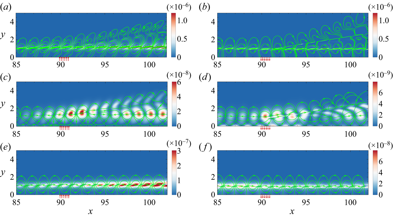
Figure 11. Flux lines of the (a,b) vortical, (c,d) acoustic and (e,f) thermal components in (a,c,e) case B3A3 with  $F=5.7\times 10^{-5}$, and (b,d,f) case S3A3 with $F=5.7\times 10^{-5}$. The control slots are all located in the range $x\in [89.9,90.9]$. The arrow directions denote the blowing or suction. The contours are coloured by each component's magnitude.
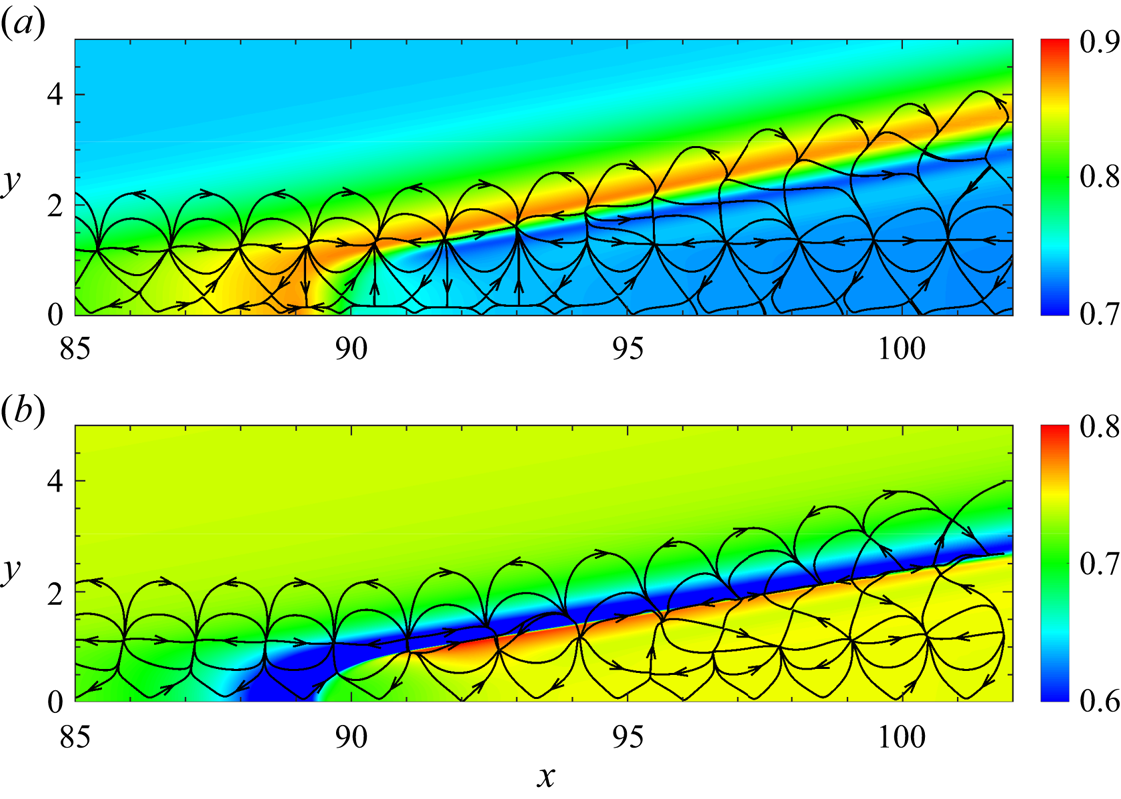
Figure 12. The acoustic component flux lines for (a) blowing control in case B3A3 with 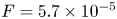 $F=5.7\times 10^{-5}$, and (b) suction control in case S3A3 with $F=5.7\times 10^{-5}$. The contours are coloured by the average pressure.
As shown in figures 11(b,d) and 12(b), although parts of the vortical and acoustic components evolve out of the boundary layer, their amplitudes are relatively small above the rarefaction wave. A distinct difference is that the inclination of the vortical and acoustic components is different with blowing and suction control. In blowing control, the component phase at a higher position is advanced, while for suction control, the phase at a higher position is delayed. This may be caused by the change in phase speed, as discussed in § 3. The thermal component also develops only within the boundary layer for suction control, as shown in figure 11(f).
For the purpose of analysing quantitatively the velocity fluctuation changes, it is more common to analyse velocities in mode evolution. Thus we derived the velocity fluctuations of the FT components from the momentum fluctuations based on the small perturbation assumption and the assumption that density/velocity fluctuation can also be decomposed into vortical, acoustic and thermal parts. Interestingly, we find that compared with momentum fluctuations used in previous investigations (Unnikrishnan & Gaitonde Reference Unnikrishnan and Gaitonde2019, Reference Unnikrishnan and Gaitonde2021), the velocity fluctuations are more reflective of the acoustic properties of the second mode from an amplitude perspective. The detailed derivations are given in Appendix C. Taking the velocity of the acoustic component as an example, it can be expressed as  $u_A' = [(\rho u)_A' - \rho _A' \bar {u})]/\bar {\rho }$. Accordingly, the momentum and velocity component evolution of the disturbance's FT components with $F=5.4\times 10^{-5}$ are shown in figures 13(a,b), respectively. The vortical component ( $B'$) has the largest amplitude and is close to the original momentum fluctuation $(\rho u)'$, while the thermal component ( $T'$) is approximately 3–5 times smaller. The acoustic component ( $A'$), on the other hand, is approximately 10 times smaller than $(\rho u)'$. This aligns with the fact that the sum of the vortical and thermal components ( $B'+T'$) closely matches $(\rho u)'$. Therefore, in terms of amplitude, the contribution of acoustic component fluctuations to momentum fluctuations is minimal. This is not the case for the velocity fluctuations, where the velocity fluctuations of the acoustic component ( $u_A'$) are actually very important for the original velocity fluctuations ( $u'$), as shown in figure 13(b). The amplitude of the acoustic component fluctuations is always of the same order of magnitude as the original velocity fluctuations. Near the synchronisation point, their amplitudes differ by a factor of 2–3 at most. Further downstream, the difference between the amplitude of the acoustic component and the original velocity fluctuation is even smaller, and by $x = 200$, the amplitude of $u_A'$ even exceeds that of $u'$. This better reflects the acoustic properties of the second mode. Additionally, the amplitudes of vortical ( $u_B'$) and thermal ( $u_T'$) component velocity fluctuations are nearly identical, but their phases are almost opposite, which can be indicated by their summation ( $u_B'+u_T'$) being much smaller than their individual amplitudes. This may better reflect the vortical–entropy coupling suggested by Crocco's theorem. The sum $u_B'+u_T'$ is of the same order of magnitude as $u'$, and as they evolve downstream, the sum develops from being almost the same as $u'$ to deviating from $u'$ until it deviates more than $u_A'$. This consists of the evolution of the disturbance from the Mack first mode (expansion of the Tollmien–Schlichting wave) to the Mack second mode (acoustic properties). Also, it should be mentioned that the velocity vector field does not have irrotational (acoustic and thermal component) or divergence-free (vortical component) properties.
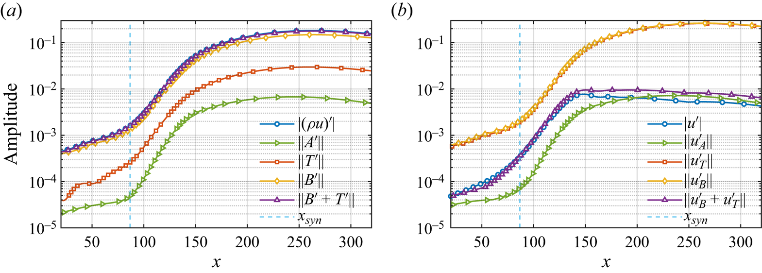
Figure 13. The streamwise evolution of (a) momentum components and (b) velocity components in MPT. The disturbance frequency is  $F=5.4\times 10^{-5}$, and the vertical dashed line marks the synchronisation point.
For instability control, figure 14 presents the FT component velocity evolution for the cases B3A3 and S3A3 with frequency  $F=5.7\times 10^{-5}$. In the vicinity of the blowing region $85< x<90$, the vortical, acoustic and thermal components all amplify rapidly, indicating that the modified base flow is more unstable. Downstream ( $90< x<93$), the acoustic and vortical components decay rapidly, while the thermal component is maintained. This is consistent with the phenomenon that some acoustic and vortical components propagate out of the boundary layer. Meanwhile, we noticed that the acoustic component oscillates near the blowing, while intriguingly, neither the vortical nor thermal components display individual oscillations; however, the sum of them demonstrates oscillations. This may be caused by the difference in their phase speeds as they pass through the compression wave. The oscillatory behaviour of the FT components results in the velocity oscillation near the blowing, which can also be observed in figure 5(b).
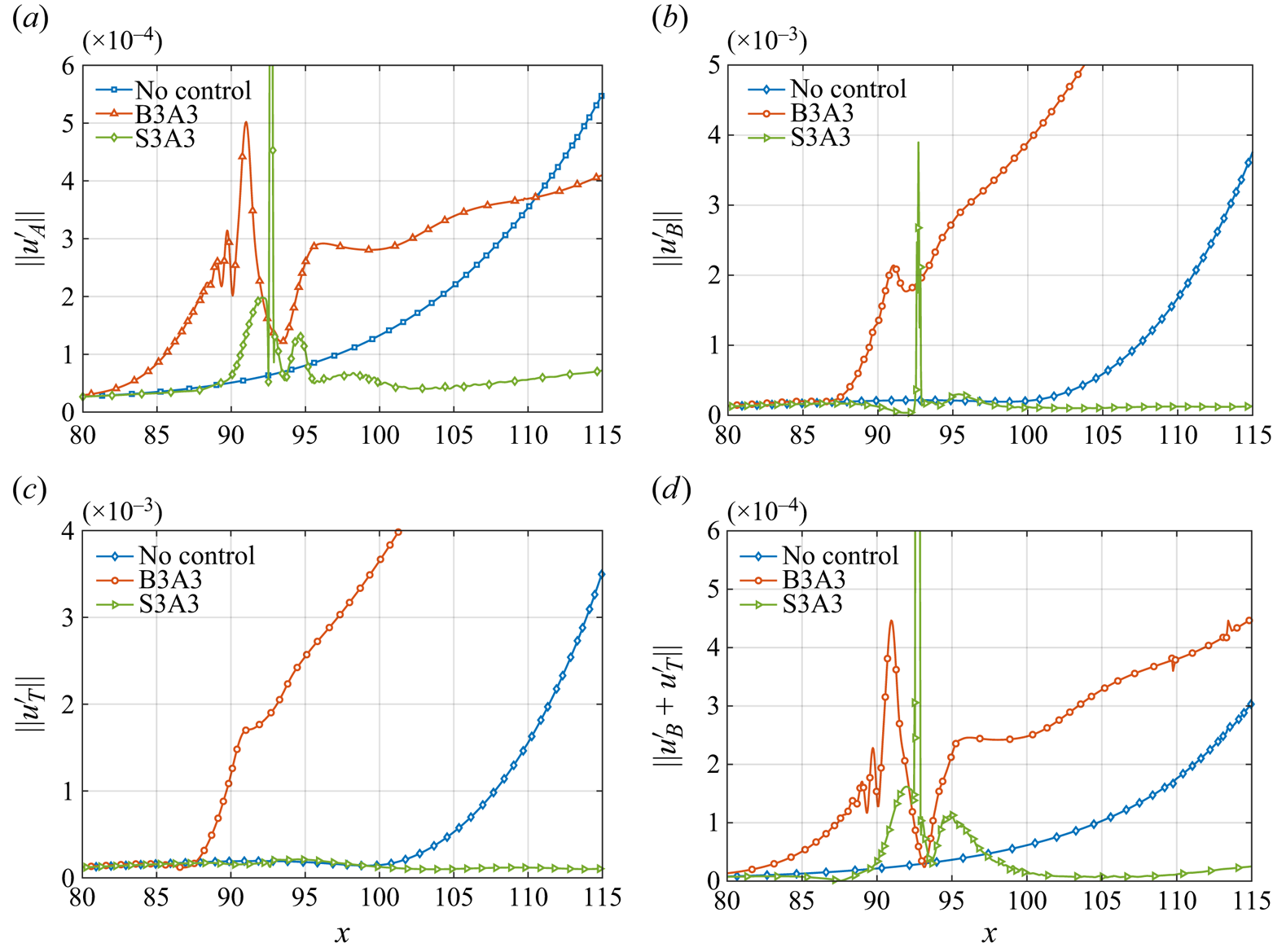
Figure 14. The streamwise evolution of (a) acoustic component, (b) vortical component, (c) thermal component, and (d) the sum of vortical and thermal components, in cases B3A3 and S3A3, with frequency  $F=5.7\times 10^{-5}$.
However, unlike blowing, the vortical, acoustic and thermal components in the vicinity of suction ( $85< x<92$, approximately) evolve in different ways. The acoustic component is promoted, the vortical component is suppressed, and the thermal component remains almost unchanged. In addition, the increasing sum of the vortical and thermal components indicates that the phase lags of the vortical and thermal components change when the disturbance passes through the rarefaction wave. Further downstream ( $x>95$), all of the FT components show a tendency to be suppressed.
5.2. Non-parallel and viscous effects
Although the MPT provides the evolution of the FT component in the vicinity of the compression/rarefaction wave, the suppression mechanism of the disturbance remains obscure, especially in understanding why the disturbance is suppressed near the suction. Consequently, the kinetic energy budget analysis is adopted to analyse the disturbance evolution, which classifies the terms corresponding to the growth of the disturbance kinetic energy into a production term  $\mathcal {P}$, a pressure term $\varPi$, a non-parallel term $\varXi$, and a viscous term $\mathcal {V}$. A detailed derivation can be found in Appendix B.
The blowing and suction control induces a stronger non-parallel effect, as mentioned in § 3, and its influence on the evolution of disturbance in the vicinity of blowing/suction needs to be clarified. Because the non-parallel effect will affect the evolution of disturbance in the boundary layer (Fasel & Konzelmann Reference Fasel and Konzelmann1990; Dong & Zhao Reference Dong and Zhao2021), it is also considered to be related to the outward development of acoustic and vortical components in the boundary layer, leading to a stabilising effect (Zhuang et al. Reference Zhuang, Wan, Ye, Luo, Liu, Sun and Lu2023). In addition, viscosity generally plays a stabilising role and is considered to have less impact on mode growth (Chen, Zhu & Lee Reference Chen, Zhu and Lee2017; Tian & Wen Reference Tian and Wen2021). However, the validity of this conclusion needs to be checked for rapidly varying base flows.
To compare the roles of each term in (B12) for different control conditions or different streamwise stations, a normalisation with  $|u_{max}'|^2$ is employed. This normalisation effectively disregards the effect of the mode amplitude on the magnitude of the viscous term, and instead highlights the effect of variations in the mode profile and the base flow on each term.
Figure 15 presents the streamwise evolution of each term for the control case B3A3 with  $F=5.7\times 10^{-5}$. Under blowing control, the destabilising effect of non-parallelism is stronger than that of base flow without control. However, in the vicinity of the blowing ( $80< x<90$), this effect acts as a stabiliser. Downstream, the destabilising effect weakens gradually. The stabilisation effect of non-parallelism is assumed to be related to the propagation of vortical and acoustic components outwards, as mentioned in § 5.1. In suction control, the non-parallel term varies drastically along the streamwise direction. To better understand the variation in the non-parallel term, figures 15(c,d) analyse the evolution of $\varXi _1$ and $\varXi _2$, two components of the non-parallel term. The first term contains the effect of the stronger local wall-normal velocity induced by blowing or suction on the energy, as the normal velocity in the boundary layer without control is smaller. The remaining term contains mainly the effect of streamwise changes in the boundary layer base flow. The term $\varXi _1$ in the blowing control suppresses mode growth, while $\varXi _1$ in the suction control promotes mode growth, as shown in figures 15(c,d). The wall-normal velocity can transport energy outside the boundary layer or inside the suction slot, and it consists of the phenomenon in the blowing control, as blowing transports part of the acoustic component out of the boundary layer. But for suction, the $\varXi _1$ promotes mode growth, which should be related to the change in the phase difference between the mode and corresponding force terms. Overall, the term $\varXi _1$ will destabilise the disturbance near the suction. As shown in figures 15(a,b), the viscous effects near the blowing/suction were all enhanced with control. The region of rapid viscosity enhancement is located in the interval where the boundary layer rapidly thickens, such as when $x$ ranges from 80 to 89 in the blowing control, and from 90 to 91 in the suction. In particular, for suction control, the viscous term increases by a factor of approximately 3.
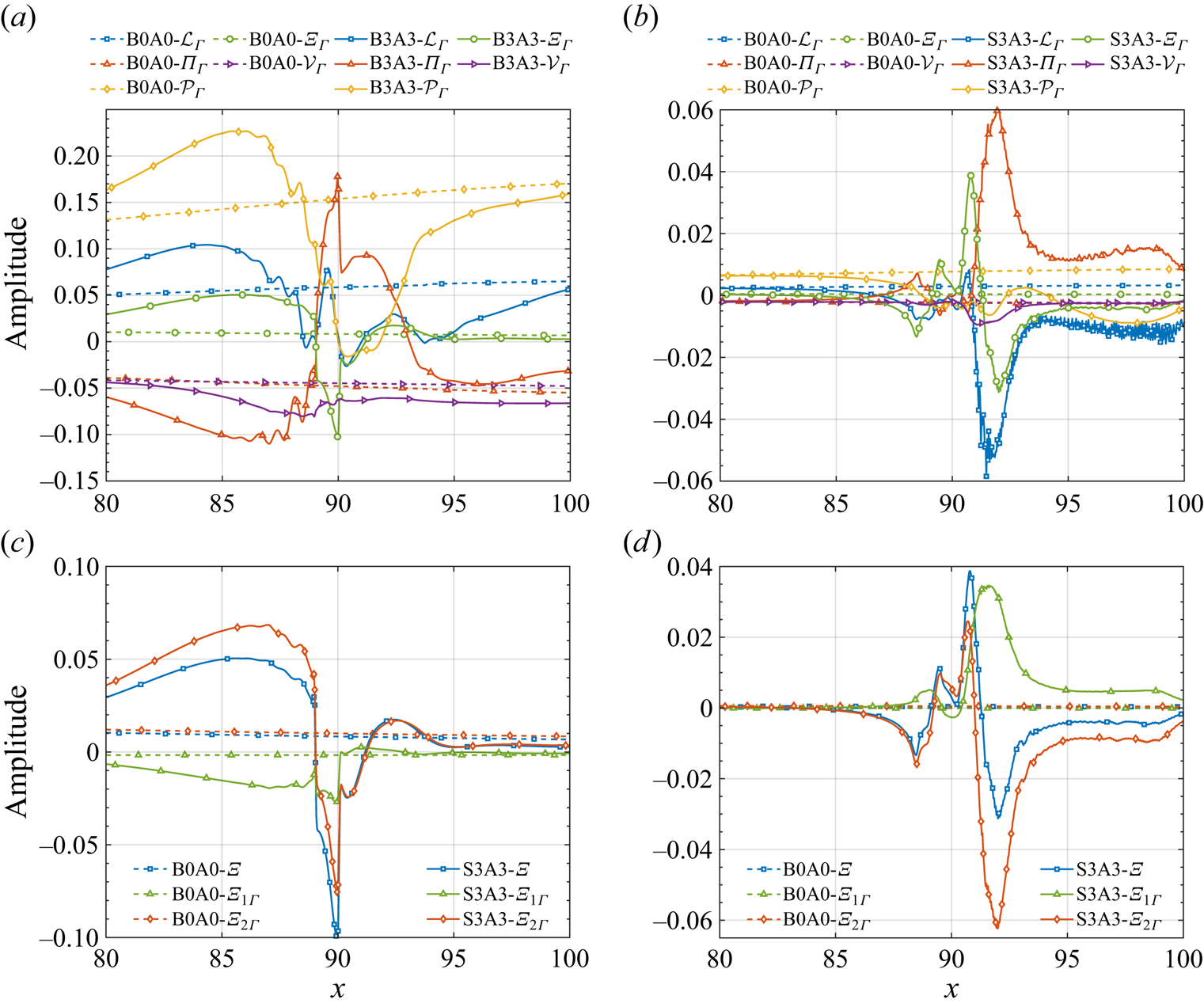
Figure 15. The streamwise evolution of  $\mathcal {L}$, $\mathcal {P}$, $\varXi$, $\varPi$ and $\mathcal {V}$ in the linear energy transfer term of (a) blowing control and (b) suction control. The streamwise evolution of $\varXi$, $\varXi _1$ and $\varXi _2$ in the non-parallel term for (c) blowing control and (d) suction control.
6. Transition delaying based on a combination of blowing and suction
In this section, we demonstrate that a combination of blowing and suction is effective in suppressing hypersonic flat plate boundary layer transitions under random incoming flow disturbances. Although blowing and suction are common tools for flow control (Fan et al. Reference Fan, Atzori, Vinuesa, Gatti, Schlatter and Li2022; Kneer, Guo & Kloker Reference Kneer, Guo and Kloker2022; Li & Zhang Reference Li and Zhang2022), they have not been found to be as effective as porous walls, rough elements, and so on, in terms of transition delaying, either experimentally or numerically. Here, we find that a suitable combination of blowing and suction can delay the transition to some extent.
Three-dimensional DNS are utilised to verify the transition delay effect. The parameters of far-field flow are the same as those in the investigation by Zhuang et al. (Reference Zhuang, Wan, Ye, Luo, Liu, Sun and Lu2023). The  $Re_l$ in the inlet of the computational domain is $Re_l=2150$, and the streamwise, wall-normal and spanwise lengths of the computation domain are $L_x = 500 \delta _0$, $L_y = 50 \delta _0$ and $L_z = 16 \delta _0$, where $\delta _0$ is the inlet boundary layer thickness. The grid resolution of the physical domain is $10450\times 220\times 240$. The mesh spacings are chosen to be $x^+ = 2.80$, $y_{wall}^+=0.43$ and $z^+ = 3.58$ to resolve the transition simulation. The wall boundary layer is chosen as an adiabatic no-slip wall surface, and the upstream, downstream, and upper boundary layer regions are the far-field boundary layer with buffer zones imposed on damp disturbances.
The random free-stream disturbance form follows that implemented in the DNS investigation by Hader & Fasel (Reference Hader and Fasel2018, Reference Hader and Fasel2022), in which the numerical results are in agreement with the experiment. However, there exist slight disparities in specific aspects. In our study, we introduce a random pressure disturbance to each grid point within the  $y$–
$y$– $z$ plane at $x = 5$, whereas previous studies (Hader & Fasel Reference Hader and Fasel2018, Reference Hader and Fasel2022) applied them within the $x$–
$x$– $y$ plane by considering a range of 5 grid points in the $x$ direction near the inlet. It should emphasised that randomness is currently introduced to the spanwise wavenumber of triggering disturbances, thereby imposing more difficulties for control. The skin friction is adopted to evaluate the transition position, calculated as
 \begin{equation} C_f = \left.\frac{2}{Ma\,Re}\,\mu\,\frac{\partial u}{\partial y} \right|_{y=0}. \end{equation}
 Figure 16(a) shows the evolution of mean skin friction coefficients ( $\bar {C}_f$) averaged over the spanwise direction and time over 100 $\delta _0/c$. This shows that $\bar {C}_f$ starts to increase at $x\approx 260$, indicating the start of the transition. Figure 16(b) presents the wall pressure disturbance, and it can be observed that the major instability includes the 2-D second mode instability upstream transition even though the forcing is randomly perturbed in the spanwise direction. To delay the transition, the blow strips are positioned at $[149.6,150.4]$ and $[219.6,220.4]$. The suction strips are positioned at $[151.2,152]$ and $[221.2,222]$. The amplitudes of blowing and suction are set to $0.1U_{\infty }$. Figure 16(c) shows the wall pressure contours with control. The 2-D second mode is significantly damped near the control strip, and downstream of the second control strip, disturbances with specific wavenumbers dominate the flow evolution until the onset of the transition. The $\bar {C}_f$ evolutions with and without control are compared in figure 16. In order to assess the effect of transition delay, the transition Reynolds numbers are defined as the location where the skin friction reaches $\frac {1}{2}(\bar {C}_{f,max}+\bar {C}_{f,min})$, where $\bar {C}_{f,max}$ and $\bar {C}_{f,min}$ are the maximum and minimum values of $\bar {C}_f$ without control. Transition locations are located at $1.71\times 10^7\ (x\approx 326)$ and $1.79\times 10^7\ (x\approx 346)$, respectively, and a transition delay of approximately $4.6\,\%$ is achieved.
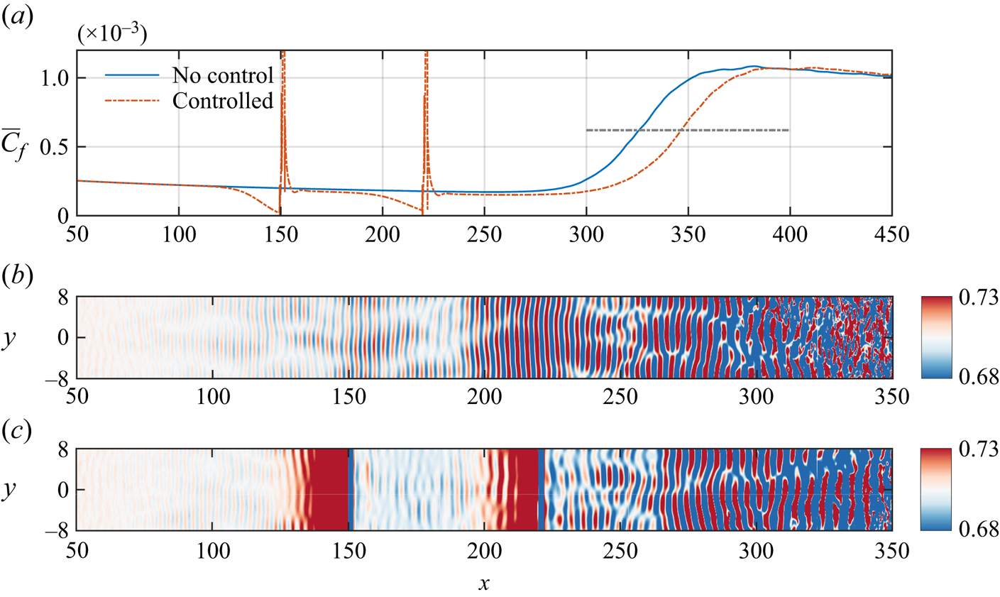
Figure 16. (a) The  $C_f$ evolution of transition flow without and with the steady blowing/suction control. The instantaneous wall pressure contours (b) without control and (c) with control.
The resolvent analysis results for base flow without control and with control are shown in figures 17(a) and 17(b), respectively. The calculation domain for the resolvent analysis is  $x\in [0,300]$, with 1000 points and 150 points in the $x$ and $y$ directions, respectively. The base flow was obtained by averaging 40 000 flow fields equally spaced in time over duration $52 \delta _0/c$, followed by averaging in the spanwise direction. As depicted in figure 17(a), the disturbance with frequency $F=3.8\times 10^{-5}$ exhibits the highest gain. Figures 17(c) and 17(d) illustrate the evolution of disturbance frequency spectra without and with control, which were obtained through 2-D FFT in time and spanwise directions. With random disturbances, there is an observed transfer of dominant mode frequency from high to low frequencies along the streamwise direction, consistent with findings from experimental studies (Bountin, Shiplyuk & Maslov Reference Bountin, Shiplyuk and Maslov2008; Laurence, Wagner & Hannemann Reference Laurence, Wagner and Hannemann2016). The well-captured frequency at $F=3.8\times 10^{-5}$ during upstream breakdown indicates that the forcing mode employed in resolvent analysis can appropriately reflect nonlinear interaction effects during this process. The critical frequency for 2-D disturbance is approximately $3.5\times 10^{-5}$, where disturbances with lower frequencies are mainly promoted, while those with higher frequencies above are suppressed. With the spanwise number increasing, the critical frequency moves to a higher frequency until $\beta \approx 7.5\times 10^{-5}$. The critical frequency for 2-D disturbance is lower than the peak frequency, and the DNS result shows a good agreement with the resolvent result, as shown in figure 17(d). The disturbances with frequencies higher than the critical frequency are notably damped, and the dominant frequencies upstream of the breakdown are frequencies lower than the critical frequency.
Figure 17. The grey background shows optimal gain with respect to  $F$ and $\beta$ for base flow (a) without control and (b) with control. The solid lines denote those contours of different $\mu _c/\mu _{uc}$, in which $\mu _c$ is the optimal gain with control, and $\mu _{uc}$ is the optimal gain without control. The frequency spectrum evolution of 2-D disturbances (c) without control and (d) with control. The dashed line marks the peak frequency of the resolvent analysis of the uncontrolled base flow.
7. Conclusion
The present study investigates systematically the control effect of constant blowing/suction with large amplitudes ranging from  $10^{-2}U_{\infty }^*$ to $10^{-1}U_{\infty }^*$ on instability and transition in a flat plate hypersonic boundary layer at Mach number 5.86. The control effects of blowing and suction flux, as well as amplitude on the hypersonic boundary layer instability, are investigated through a combination of DNS and resolvent analysis. The critical frequency is utilised to measure the blowing and suction control effects, and mode suppression occurs with its frequency higher/lower than the critical frequency with blowing/suction control. When the blowing flux is relatively small, the critical frequency for 2-D disturbance is closely aligned with the synchronisation frequency; however, increasing the blowing flux significantly shifts the critical frequency towards lower frequencies. On the other hand, suction control leads to a shift of the critical frequency towards higher frequencies.
For the oblique wave, the increase of spanwise wavenumber will lead to a higher critical frequency in both blowing and suction control. Meanwhile, if the spanwise wavenumber increases, then the suppression effects would become weaker, and mode suppression bandwidth diminishes/increases in blowing/suction control.
Moreover, an increase in the maximum disturbance suppression effect is observed with higher blowing flux levels. At a fixed level of flux, variations in blowing or suction amplitude have relatively minor impacts on disturbance suppression. Additionally, based on resolvent analysis, it is found that while most sensitive regions of the modified base flow remain concentrated around the GIP under control, downstream boundary layer lift also causes lifting of the GIP due to blowing. Suction control predominantly affects regions around the GIP, which results in the formation of new sensitive regions near suction.
The growth of the disturbance upstream or downstream of the control is influenced primarily by the stability of the boundary layer, which is determined by its varying thickness. To analyse the local evolution mechanism of the disturbance, we employ MPT and kinetic energy budget analysis. Blowing induces the evolution of acoustic components along the compression wave outside the boundary layer. In contrast, suction control does not have this effect. We find that velocity fluctuations derived from momentum fluctuations in MPT better reflect the nature of the second mode as an acoustic mode. Near blowing, there are differences in phase speeds between vortical and thermal components, causing oscillations in velocity fluctuation. The analysis of the kinetic energy budget reveals that the non-parallel effect becomes stronger near the blowing and suction. The non-parallel effect, which relates directly to the wall-normal velocity, stabilises the disturbance near blowing, and destabilises it near suction. The impact of viscosity becomes more pronounced in regions characterised by rapid thickening of the boundary layer due to blowing/suction control.
The effectiveness of transition control using three-dimensional DNS is investigated, as blowing and suction have been found to effectively suppress disturbances. Random pressure disturbances in a  $y$–
$y$– $z$ plane located upstream of the computational domain were used to trigger a flat plate boundary layer transition with Mach number 5.86. It was observed that the average transition Reynolds number increased by 4.6 %. Resolvent analysis reveals that the base flow control stabilised the disturbances within specific frequency and wavenumber ranges during the early stages of transition. Overall, blowing and suction show the potential for delaying transitions, and future optimisation of amplitude and distribution using an optimisation method could further enhance their transition control effect.
Acknowledgements
The numerical computations were performed at Hefei Advanced Computing Center.
Funding
This work is sponsored by the National Natural Science Foundation of China under grant nos 12172351, 92252202, 12322210, 92052301 and 12388101, as well as the Fundamental Research Funds for the Central Universities.
Declaration of interests
The authors report no conflict of interest.
Appendix A. Momentum potential theory
Choosing  $\rho \boldsymbol {v}$ as the primary independent variable, the momentum vector field can be expressed as a linear superposition of unique solenoidal and irrotational components by the Helmholtz decomposition
 \begin{equation} \rho \boldsymbol{v} = \bar{B} - \boldsymbol{\nabla} \bar{\psi} + B' +\boldsymbol{\nabla} \psi' , \quad \boldsymbol{\nabla} \boldsymbol{\cdot} \bar{B} = \boldsymbol{\nabla} \boldsymbol{\cdot} B' = 0, \end{equation}
where  $\bar {B}$ and $B'$ denote the mean and fluctuating parts of the rotational component, and $\bar {\psi }$ and $\psi '$ are the mean and fluctuating parts of the scalar momentum potential.
For a time-stationary flow, if  $\bar \psi$ is solenoidal and thus equal to zero, then the continuity equation is equivalent to a Poisson equation
 \begin{equation} \nabla^2\psi^{\prime}= \frac{\partial \rho^{\prime}}{\partial t}.\end{equation}
For the perfect gas, considering the constitutive relationship, one can obtain
 $$\begin{gather} \delta \rho=\rho_p\,\delta p + \rho_S\,\delta S, \end{gather}$$
 $$\begin{gather}\rho_p\equiv(\partial\rho/\partial p)_S\equiv1/c^2,\quad \rho_S\equiv(\partial\rho/\partial S)_p, \end{gather}$$
where  $S$ denotes the entropy. Inserting (A3) and (A4a,b) into (A2) gives
 \begin{equation} \nabla^2\psi^{\prime}=\frac{1}{c^2}\,\frac{\partial p \prime}{\partial t} + \rho_S\,\frac{\partial S ^\prime}{\partial t}. \end{equation}
 Then  $\psi '$ can be defined as the sum of acoustic ( $\psi _{A}'$) and entropic (or thermal, $\psi _{T}'$) components
 \begin{equation} \psi^{\prime}\equiv \psi_{A}^{\prime}+\psi_{T}^{\prime}, \quad \frac{\partial^2\psi^{\prime}_A}{\partial x^2_i} \equiv\frac{1}{c^{2}}\,\frac{\partial p^{\prime}}{\partial t}, \quad \frac{\partial^2\psi^{\prime}_T}{\partial x^2_i} \equiv\rho_S\,\frac{\partial S^{\prime}}{\partial t}. \end{equation}
For convenience, we also use the notation  $A'$ and $T'$ to present the acoustic and thermal components.
Appendix B. Kinetic energy budget analysis
Following the kinetic energy transfer derivations in the investigation by Chen et al. (Reference Chen, Zhu and Lee2017), considering a small disturbance  $q'$ with spatial structure as $\tilde {q}(x,y)\, {\rm e}^{{\rm i} \omega t}$, the streamwise $u$-momentum equation can be rewritten as
 \begin{equation} \bar{\rho}\,\frac{{\rm D} \tilde{u}}{{\rm D} t} = \mathcal{L}_{\tilde{u}}.\end{equation}
The superscript  $\,\tilde {}\, $ in this appendix indicates the mode spatial function, and $\mathcal {L}_{\tilde {u}}$ indicates the linear terms. Multiply (B7) by $\tilde {u}^*$ (the complex conjugate of $\tilde {u}$), and the two equations are added to obtain
 \begin{equation} \rho_0\,\frac{{\rm D}\,|\tilde{u}|^2}{{\rm D} t} = \tilde{u}^*\mathcal{L}_{\tilde{u}} + {\rm c.c.}\end{equation}
Performing the same operations on the  $v$-momentum equation gives the kinetic energy equation as
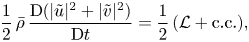 \begin{equation} \frac{1}{2}\,\bar{\rho}\,\frac{{\rm D} (|\tilde{u}|^2 + |\tilde{v}|^2)}{{\rm D} t} = \frac{1}{2}\,(\mathcal{L} + {\rm c.c.}), \end{equation}
where
 \begin{equation} \mathcal{L} = \tilde{u}^*\mathcal{L}_{\tilde{u}} + \tilde{v}^*\mathcal{L}_{\tilde{v}} + {\rm c.c.} \end{equation}
Here, we define the reduced kinetic energy of a unit volume for one mode as
 \begin{equation} e \equiv \tfrac{1}{2} {\bar{\rho}}(|\tilde{u}|^2+|\tilde{v}|^2).\end{equation}
The linear term  $\mathcal {L}$ can be further divided to
 \begin{equation} \mathcal{L} = \mathcal{P} + \varXi + \varPi +\mathcal{V},\end{equation}
where
 \begin{gather} \mathcal{P}=-\bar{\rho} \tilde{u}^* \tilde{v}\, \frac{\partial \bar{u}}{\partial y}+\text{c.c.}, \end{gather}
 \begin{gather} \varXi=-\tilde{u}^* \bar{\rho} \tilde{u}\, \frac{\partial \bar{u}}{\partial x} -\left(\tilde{u}^*\,\frac{\partial \tilde{u}}{\partial y} + \tilde{v}^*\, \frac{\partial \tilde{v}}{\partial y}\right) \bar{\rho} \bar{v} - \tilde{v}^* \bar{\rho} \tilde{u}\,\frac{\partial \bar{v}}{\partial x} - \tilde{v}^* \bar{\rho} \tilde{v}\,\frac{\partial \bar{v}}{\partial y} \nonumber\\ \quad - \tilde{u}^* \tilde{\rho} \left(\bar{u}\,\frac{\partial \bar{u}}{\partial x} + \bar{v}\,\frac{\partial \bar{u}}{\partial y}\right) - \tilde{v}^* \tilde{\rho}\left(\bar{u}\,\frac{\partial \bar{v}}{\partial x} + \bar{v}\,\frac{\partial \bar{v}}{\partial y}\right)+\text{c.c.}, \end{gather}
 \begin{gather} \varPi=-\tilde{u}^*\,\frac{\partial \tilde{p}}{\partial x}-\tilde{v}^*\,\frac{\partial \tilde{p}}{\partial y} +\text{c.c.}.\end{gather}
Here,  $\mathcal {P}$ is the production, $\varXi$ is regarded as the energy transfer associated with the non-parallel term, $\varPi$ is the pressure diffusion/dilatation, and $\mathcal {V}$ is the energy transfer related to viscous terms. The term $\varXi$ is further split into two parts, as follows:
 \begin{align} \varXi_1&=- \bar{\rho} \bar{v} \left(\tilde{u}^*\, \frac{\partial \tilde{u}}{\partial y} + \tilde{v}^*\,\frac{\partial \tilde{v}}{\partial y}\right)- \tilde{v}^* \bar{\rho} \tilde{u}\,\frac{\partial \bar{v}}{\partial x} - \tilde{v}^* \tilde{\rho} \bar{u}\,\frac{\partial \bar{v}}{\partial x} - \tilde{v}^* \bar{\rho} \tilde{v}\,\frac{\partial \bar{v}}{\partial y}\nonumber\\ &\quad - \tilde{u}^* \tilde{\rho} \bar{v}\,\frac{\partial \bar{u}}{\partial y} + \text{c.c.}, \end{align}
 \begin{gather} \varXi_2=- \tilde{u}^* \bar{\rho} \tilde{u}\,\frac{\partial \bar{u}}{\partial x} - \tilde{v}^* \bar{\rho} \tilde{v}\,\frac{\partial \bar{v}}{\partial y} - \tilde{u}^* \tilde{\rho} \bar{u}\,\frac{\partial \bar{u}}{\partial x} + {\rm c.c.}\end{gather}
Integrating (B9) with respect to the wall-normal coordinate gives
 \begin{equation} \mathcal{L}_{\varGamma} \equiv \int_0^{\infty} \mathcal{L} \,\mathrm{d} y. \end{equation}
Similar operations on (B11), (B12), (B14) and (B15) give  $(1/2)(\bar{\rho}De/Dt)_{\gamma}$, $\mathcal {P}_\varGamma$, $\varXi _\varGamma$, $\varPi _\varGamma$ and $\mathcal {V}_\varGamma$.
Appendix C. Derivation of the velocity fluctuations of FT components in MPT
In MPT, momentum fluctuations are decomposed into the sum of mean momentum, vortical component, acoustic component and thermal component:
 \begin{equation} \rho u=\bar{\rho u}+(\rho u)_A^{\prime}+(\rho u)_B^{\prime}+(\rho u)_T^{\prime}. \end{equation}
Further, with a simple assumption that the density and velocity fluctuations can also be split into the mean density/velocity part, vortical part, acoustic part and thermal part, we have
 \begin{equation} \rho=\bar{\rho}+\rho_A^{\prime}+\rho_B^{\prime}+\rho_T^{\prime} \end{equation}
and
 \begin{equation} u=\bar{u}+u_A^{\prime}+u_B^{\prime}+u_T^{\prime}. \end{equation}
The momentum can then be rewritten as
 \begin{align} \rho u&=(\bar{\rho}+\rho_A^{\prime}+\rho_B^{\prime}+\rho_T^{\prime}) (\bar{u}+u_A^{\prime}+u_B^{\prime}+u_T^{\prime}) \nonumber\\ &=\bar{\rho} \bar{u}+\bar{\rho} u_A^{\prime}+\rho_A^{\prime} \bar{u}+\bar{\rho} u_B^{\prime}+\rho_B^{\prime} \bar{u}+\rho_T^{\prime} \bar{u}+\bar{\rho} u_T^{\prime} \nonumber\\ &\quad +(\rho_A^{\prime}+\rho_B^{\prime}+\rho_T^{\prime}) (u_A^{\prime}+u_B^{\prime}+u_T^{\prime}). \end{align}
When the amplitudes of density and velocity fluctuations are small, the higher-order terms can be neglected. Then we combine terms on the right-hand side of the equation,
 \begin{equation} \left.\begin{array}{l@{}} (\rho u)_A^{\prime}=\bar{\rho} u_A^{\prime}+\rho_A^{\prime} \bar{u}, \\ (\rho u)_B^{\prime}=\bar{\rho} u_B^{\prime}+\rho_B^{\prime} \bar{u}, \\ (\rho u)_T^{\prime}=\bar{\rho} u_T^{\prime}+\rho_T^{\prime} \bar{u}, \end{array}\right\}\end{equation}
so
 \begin{equation} u_A' = \frac{(\rho u)_A' - \rho_A' \bar{u}}{\bar{\rho}},\quad u_B' = \frac{(\rho u)_B' - \rho_B' \bar{u}}{\bar{\rho}},\quad u_T' = \frac{(\rho u)_T' - \rho_T' \bar{u}}{\bar{\rho}}.\end{equation}
We need to obtain each component of density fluctuation. Based on the continuity equation, we have
 \begin{equation} \left.\begin{array}{l@{}} \displaystyle \dfrac{\partial \rho_A'}{\partial t} = \dfrac{\partial (\rho u)'_A}{\partial x} +\dfrac{\partial (\rho v)'_A}{\partial y}, \\ \displaystyle \dfrac{\partial \rho_B'}{\partial t} = \dfrac{\partial (\rho u)'_B}{\partial x} +\dfrac{\partial (\rho v)'_B}{\partial y}, \\ \displaystyle \dfrac{\partial \rho_T'}{\partial t} = \dfrac{\partial (\rho u)'_T}{\partial x} +\dfrac{\partial (\rho v)'_T}{\partial y}. \end{array}\right\}\end{equation}
Considering the disturbance with a specific frequency, the variables can be written in the form  $q'=\hat {q} \, \textrm {e}^{\textrm {i}\omega t}$ (where $\tilde {q}$ is a complex number, and $q$ can be $\rho _A, u_A, (\rho u)_A,\ldots\, $. ). Then taking the Fourier transform on both sides of (C7), we have
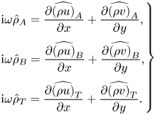 \begin{equation} \left.\begin{array}{l@{}} \displaystyle {\rm i}\omega \hat{\rho}_A = \dfrac{\partial \widehat{(\rho u)}_A}{\partial x} +\dfrac{\partial \widehat{(\rho v)}_A}{\partial y}, \\ \displaystyle {\rm i}\omega\hat{\rho}_B = \dfrac{\partial \widehat{(\rho u)}_B}{\partial x} +\dfrac{\partial \widehat{(\rho v)}_B}{\partial y}, \\ \displaystyle {\rm i}\omega \hat{\rho}_T = \dfrac{\partial \widehat{(\rho u)}_T}{\partial x} +\dfrac{\partial \widehat{(\rho v)}_T}{\partial y}. \end{array}\right\}\end{equation}
 Taking  $\hat {\rho }$ in (C8) into (C6a–c), we have
 \begin{equation} \left.\begin{array}{l@{}} \displaystyle \hat{u}_A = \dfrac{1}{\bar{\rho}} \left[ \widehat{(\rho u)}_A - \dfrac{\bar{u}}{{\rm i}\omega}\left(\dfrac{\partial \widehat{(\rho u)}_A}{\partial x} +\dfrac{\partial \widehat{(\rho v)}_A}{\partial y}\right) \right],\\ \displaystyle \hat{u}_B = \dfrac{1}{\bar{\rho}} \left[ \widehat{(\rho u)}_B - \dfrac{\bar{u}}{{\rm i}\omega}\left(\dfrac{\partial \widehat{(\rho u)}_B}{\partial x} +\dfrac{\partial \widehat{(\rho v)}_B}{\partial y}\right) \right],\\ \displaystyle \hat{u}_T = \dfrac{1}{\bar{\rho}} \left[ \widehat{(\rho u)}_T - \dfrac{\bar{u}}{{\rm i}\omega}\left(\dfrac{\partial \widehat{(\rho u)}_T}{\partial x} +\dfrac{\partial \widehat{(\rho v)}_T}{\partial y}\right) \right] . \end{array}\right\}\end{equation}
Taking the 2-norm on both sides of (C9), the amplitudes of the velocity fluctuations of acoustic, vortical and thermal components are obtained:
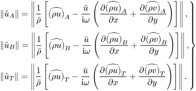 \begin{equation} \left.\begin{array}{l@{}} \displaystyle \| \hat{u}_A \| = \left\| \dfrac{1}{\bar{\rho}} \left[ \widehat{(\rho u)}_A - \dfrac{\bar{u}}{{\rm i}\omega}\left(\dfrac{\partial \widehat{(\rho u)}_A}{\partial x} +\dfrac{\partial \widehat{(\rho v)}_A}{\partial y}\right) \right] \right\|,\\ \displaystyle \| \hat{u}_B \| = \left\| \dfrac{1}{\bar{\rho}} \left[ \widehat{(\rho u)}_B - \dfrac{\bar{u}}{{\rm i}\omega}\left(\dfrac{\partial \widehat{(\rho u)}_B}{\partial x} +\dfrac{\partial \widehat{(\rho v)}_B}{\partial y}\right) \right] \right\|,\\ \displaystyle \| \hat{u}_T \| = \left\| \dfrac{1}{\bar{\rho}} \left[ \widehat{(\rho u)}_T - \dfrac{\bar{u}}{{\rm i}\omega}\left(\dfrac{\partial \widehat{(\rho u)}_T}{\partial x} +\dfrac{\partial \widehat{(\rho v)}_T}{\partial y}\right) \right] \right\|. \end{array}\right\} \end{equation}


