


1. Introduction
Particle motions induced by low-Reynolds-number flows and vice versa have been investigated since the time of Stokes (Reference Stokes1851), and remain of fundamental interest in many fields including colloid science, phoresis, active microswimmers, sedimenting systems and suspension rheology. Understanding the dynamics of particles with arbitrary and irregular geometries in Stokes flow is of paramount importance. Perturbative approaches, such as Brenner's (Reference Brenner1963, Reference Brenner1964b,Reference Brennerc,Reference Brennerd, Reference Brenner1966), are limited to small deformations from a regular (usually spherical) geometry.
The boundary element method (BEM) (Pozrikidis Reference Pozrikidis1992; Muldowney & Higdon Reference Muldowney and Higdon1995; Pozrikidis Reference Pozrikidis2002; Kim & Karrila Reference Kim and Karrila2005) is a popular numerical method for such problems. This method descends from classical Green function methods, solving a boundary integral equation which couples velocity and surface traction, but using discretization methods borrowed from the finite-element method. Only the boundary needs to be meshed. However, particles with surface roughness, sharp edges or high curvature require meshes of correspondingly high resolution.
Analytical approaches to irregular geometries are mesh-free, but they are generally limited to slightly deformed spheres (Brenner Reference Brenner1964a; Ripps & Brenner Reference Ripps and Brenner1967; Happel & Brenner Reference Happel and Brenner1983; Palaniappan Reference Palaniappan1994; Mohan & Brenner Reference Mohan and Brenner2006). In seminal work, Brenner (Reference Brenner1964a) developed a perturbative approach to obtain the velocity field around a deformed sphere using Lamb's general solution of the Stokes equation (Lamb Reference Lamb1932). The calculations grow rapidly more complicated, and therefore impractical, at higher orders of perturbation. One brilliant aspect of Brenner's method which we will borrow, however, is the mapping of a velocity field over the surface of a radially deformed sphere to a hypothetical reference sphere. This mapping turns the problem of the deformed sphere into that of solving the flow field about a reference sphere with a prescribed surface velocity field.
In this paper, we develop a non-perturbative spectral method for the flow field exterior to a highly deformed sphere. Inspired by the harmonic nature of the pressure in the Stokes equation, we define two spectra of Lamb modes. The velocity and pressure fields in the exterior domain are expressed as linear combinations of these modes, with expansion coefficients obtained by weighted integration of the surface velocity field. For velocities directly given on a sphere, for instance, a slip velocity around a self-phoretic spherical particle, use of these modes is direct and easy. To deal with velocities given on a highly, but radially, deformed spherical surface, we adapt Brenner's mapping technique to develop a formalism reducing the problem to the solution of a set of linear algebraic equations. This ability to deal with data specified on a non-spherical surface distinguishes our method from the otherwise similar approach of Pak & Lauga (Reference Pak and Lauga2014).
We test the method by computing hydrodynamic radii for a set of spheres deformed in various ways and degree, pictured in figure 1. Agreement with boundary element calculations is good. The method is then extended to calculate the propulsion speed of self-phoretic spheroids with surface flux of a driving field in source/sink or source/inert configuration, in the limit of the thin interfacial layer.

Figure 1. (a) Streamlines for flow past a selection of shapes. (b) Geometries on which the spectral method was tested. Depicted geometries are given by  ${ \boldsymbol r}_S = { \boldsymbol r}_0(1+ \delta \cos n\theta )$ for a range of
  $\delta$ and
  $n$, indicated at left and on top, respectively. The number beneath each shape is its relative hydrodynamic radius, computed via (4.1).
2. Basis and development of the method
This section discusses the expansion of fluid velocity and pressure fields in Lamb modes (Lamb Reference Lamb1932). These modes are defined everywhere on three-space with the origin deleted and tend to zero at infinity, hence are appropriate for exterior flow problems.
2.1. Problem formulation
We are interested in the velocity ( $\boldsymbol {u}$) and pressure (
 $p$) fields in a fluid exterior to a surface
  $S$, on which the velocity is specified arbitrarily. The fields are governed by the Stokes and continuity equations
 \begin{equation} \mu \nabla^{2} \boldsymbol{u} = \boldsymbol{\nabla} p, \quad \boldsymbol{\nabla} \boldsymbol{\cdot} \boldsymbol{u} = 0, \end{equation}
where  $\mu$ is viscosity and
  ${ \boldsymbol {u}}$ is assumed to tend to zero at infinity. The surface
  $S$ is given in spherical coordinates
  $(r, \theta, \phi )$ by
 \begin{equation} \boldsymbol r_s(\theta) = \boldsymbol r_0[1 + \delta \xi(\theta)].\end{equation}
Hence,  $S$ is a radial, axisymmetric, deformation of a centred reference sphere
  $S_0$ with radius
  $\boldsymbol r_0$. The deformation is parameterized in terms of a ‘shape’ function
  $\xi (\theta )$ and a magnitude
  $\delta$. We do not expand in powers of
  $\delta$ as one would in a perturbative approach, but we are still interested in how the flow changes with increasing deformation. However, the Lamb modes treated in the next few subsections are independent of this parameterization or any particular particle surface.
2.2. Lamb spectral modes
A Stokes flow pressure field is harmonic,  $\nabla ^{2} p = 0$, and, if axisymmetric, can be expanded in modes
  $p_\ell \sim r^{-(\ell +1)}\text {P}_{\ell }(\cos \theta )$ where
  $\text {P}_{\ell }$ is the Legendre polynomial of degree
  $\ell$, and
  $\hat{\boldsymbol{e}}_{r}$ and
  $\hat{\boldsymbol{e}}_{\theta}$ are unit vectors in the indicated directions. An analogous expansion of the velocity field in terms of Legendre polynomials is based on the orthogonal basis of vector-valued functions
 \begin{equation} \ell \ge 0 :
\boldsymbol{P}^{[1]}_\ell =
\text{P}_\ell(\cos\theta)\hat{\boldsymbol{e}}_{r}, \quad
\ell \ge 1: \boldsymbol{P}^{[2]}_\ell = \partial_\theta
\text{P}_\ell(\cos\theta)\hat{\boldsymbol{e}}_{\theta} =
\text{P}_{\ell}^{1}(\cos\theta)\hat{\boldsymbol{e}}_{\theta},
\end{equation}
\begin{equation} \ell \ge 0 :
\boldsymbol{P}^{[1]}_\ell =
\text{P}_\ell(\cos\theta)\hat{\boldsymbol{e}}_{r}, \quad
\ell \ge 1: \boldsymbol{P}^{[2]}_\ell = \partial_\theta
\text{P}_\ell(\cos\theta)\hat{\boldsymbol{e}}_{\theta} =
\text{P}_{\ell}^{1}(\cos\theta)\hat{\boldsymbol{e}}_{\theta},
\end{equation}
where  $\text {P}_{\ell }^{1}$ is the associated Legendre polynomial of degree
  $\ell$ and order 1. The relevant inner product on real vector-valued functions of the polar angle
  $\theta$ is
 \begin{equation} \langle\, {\boldsymbol f} | {\boldsymbol g} \rangle = \int_0^{\rm \pi} {\boldsymbol f}\boldsymbol{\cdot}{\boldsymbol g} \sin\theta \, {\rm d} \theta. \end{equation}
The orthogonal basis is normalized as  $\langle \boldsymbol {P}_{\ell }^{[1]} | \boldsymbol {P}_{\ell }^{[1]} \rangle = {2}/({2\ell +1})$,
  $\langle \boldsymbol {P}_{\ell }^{[2]} | \boldsymbol {P}_{\ell }^{[2]} \rangle = {2\ell (\ell +1)}/({2\ell +1})$. The basis functions
  $\boldsymbol {P}^{[1]}_\ell$ and
  $\boldsymbol {P}^{[2]}_\ell$ are proportional to the vector spherical harmonics (Morse & Feshbach Reference Morse and Feshbach1953)
  $Y_{\ell,m}\hat {r}$ and
  $r{\boldsymbol {\nabla }}Y_{\ell,m}$, respectively, with
  $m=0$. While
  $\boldsymbol {P}_\ell ^{[\alpha ]}$ does not solve (2.1a,b), appropriate modes can be obtained with the ansatz
  ${ \boldsymbol {u}} ({ \boldsymbol r})= \sum _{\alpha }\sum _{\ell } C_\ell ^{[\alpha ]} r^{-n(\alpha,\ell )} \boldsymbol {P}_\ell ^{[\alpha ]}$, where
  $C_\ell ^{[\alpha ]}$ is an expansion coefficient and
  $\alpha = 1$ or 2. There are two families: (Kessler, Finken & Seifert Reference Kessler, Finken and Seifert2008) biharmonic (
 $\nabla ^{4} { \boldsymbol {u}}_\ell ^{[1]}({ \boldsymbol r}) = 0$ and
  $\nabla ^{2}{ \boldsymbol {u}}_\ell ^{[1]}({ \boldsymbol r}) \not =0$) Lamb modes
 \begin{equation} \ell \ge 1: \quad \begin{array}{l} { \boldsymbol{u}}_\ell^{[1]}({ \boldsymbol r}) = \left(\dfrac{r_0}{r} \right)^{\ell}[ \ell(\ell+1)\boldsymbol{P}^{[1]}_\ell(\cos\theta) - (\ell-2)\boldsymbol{P}^{[2]}_\ell(\cos\theta)],\\ {p}_\ell^{[1]} ({ \boldsymbol r}) = 2\ell(2\ell-1) \left(\dfrac{\mu}{r_0}\right) \left(\dfrac{r_0}{r} \right)^{\ell+1}\text{P}_\ell(\cos\theta), \end{array}\end{equation}
and harmonic ( $\nabla ^{2}{ \boldsymbol {u}}_\ell ^{[2]}({ \boldsymbol r}) =0$) Lamb modes
 \begin{equation} \ell \ge 0: \quad \begin{array}{l} { \boldsymbol{u}}_\ell^{[2]}({ \boldsymbol r}) = \left(\dfrac{r_0}{r} \right)^{\ell+2} [-(\ell+1)\boldsymbol{P}^{[1]}_\ell(\cos\theta) + \boldsymbol{P}^{[2]}_\ell(\cos\theta)],\\ {p}_\ell^{[2]} ({ \boldsymbol r}) = 0. \end{array} \end{equation}
Since the Stokes equation is linear, using the modes (2.5) and (2.6), we can write a general solution of flow field around a solid particle:
 \begin{equation} \begin{pmatrix} { \boldsymbol{u}}({ \boldsymbol r}) \\ {p}({ \boldsymbol r}) \end{pmatrix} = \sum_{\alpha} \sum_{\ell} A_{\ell}^{[\alpha]} \begin{pmatrix} { \boldsymbol{u}}_\ell^{[\alpha]}({ \boldsymbol r}) \\ p_\ell^{[\alpha]}({ \boldsymbol r}) \end{pmatrix},\end{equation}
where  $A_{\ell }^{[\alpha ]}$ are expansion coefficients. Since only the biharmonic modes contribute to pressure, one can simply ignore
  $p_\ell ^{[2]}({ \boldsymbol r})$ in practice.
2.3. Extrapolating from a sphere
Suppose the velocity  ${ \boldsymbol {u}}({ \boldsymbol r}_0)$ on the surface of the reference sphere
  $S_0$ of radius
  $r_0$ is given. In order to continue this off the sphere, we need appropriate coefficients
  $A_\ell ^{[\alpha ]}$ for the expansion (2.7). However, unlike the
  ${\boldsymbol P}_\ell ^{[\alpha ]}$, the
  ${ \boldsymbol {u}}_\ell ^{[\alpha ]}$ are not orthogonal with respect to the inner product (2.4). Complementary dual vectors, satisfying
  $\langle {\boldsymbol D}_{\ell _1}^{[\alpha _1]} | {\boldsymbol {u}}_{\ell _2}^{[\alpha _2]} ({ \boldsymbol r}_0)\rangle = \delta _{\ell _1\ell _2}\delta _{\alpha _1\alpha _2}$ are therefore useful, since the expansion coefficients can then be obtained as
  $A_{\ell }^{[\alpha ]} = \langle {\boldsymbol D}_{\ell }^{[\alpha ]} | { \boldsymbol {u}} ({ \boldsymbol r}_0)\rangle$. These dual vectors are given by
 $$\begin{gather} {\boldsymbol D}_\ell^{[1]}(\cos\theta) = \frac{2\ell+1}{4 \ell(\ell+1)}[ \ell\boldsymbol{P}^{[1]}_\ell(\cos\theta) + \boldsymbol{P}^{[2]}_\ell(\cos\theta)] \quad (\ell \geq 1), \end{gather}$$
 $$\begin{gather}{\boldsymbol D}_\ell^{[2]}(\cos\theta) = \frac{2\ell+1}{4(\ell+1)}[ (\ell-2)\boldsymbol{P}^{[1]}_\ell(\cos\theta) + \boldsymbol{P}^{[2]}_\ell(\cos\theta)] \quad (\ell \geq 0). \end{gather}$$
Using these, for velocity and pressure fields around a solid sphere we have
 \begin{equation} \begin{pmatrix} { \boldsymbol{u}}({ \boldsymbol r}) \\ {p}({ \boldsymbol r}) \end{pmatrix} = \sum_{\alpha} \sum_{\ell} \langle {\boldsymbol D}_{\ell}^{[\alpha]} | { \boldsymbol{u}} ({ \boldsymbol r}_0)\rangle \begin{pmatrix} {\boldsymbol{u}}_{\ell}^{[\alpha]}({ \boldsymbol r}) \\ {p}_{\ell}^{[\alpha]}({ \boldsymbol r}) \end{pmatrix}.\end{equation}
2.4. Spherical examples
We illustrate the utility of (2.10) with two basic problems for a spherical surface.
(a) Rigid body motion. For a uniform velocity on a spherical surface, we have from (2.5) and (2.6)
 \begin{equation} { \boldsymbol{u}}_{{rigid}}({ \boldsymbol r}_0)= \hat{\boldsymbol{e}}_{z} = \text{P}_1(\cos\theta)\hat{\boldsymbol{e}}_{r} + \text{P}_1^{1}(\cos\theta)\hat{\boldsymbol{e}}_{\theta} = \tfrac{3}{4} { \boldsymbol{u}}_1^{[1]}({ \boldsymbol r}_0)+ {\tfrac{1}{4}} { \boldsymbol{u}}_1^{[2]}({ \boldsymbol r}_0). \end{equation}
Using (2.10) we recover the classical Stokes solution (Leal Reference Leal2007)
 \begin{align} { \boldsymbol{u}}_{rigid}({ \boldsymbol r}) & = \frac{3}{4} { \boldsymbol{u}}_1^{[1]}({ \boldsymbol r}) + \frac{1}{4}{ \boldsymbol{u}}_1^{[2]}({ \boldsymbol r}) \nonumber\\ & =\frac{1}{2} \cos\theta \left[ 3 \left(\frac{r_0}{r}\right) - \left(\frac{r_0}{r}\right)^{3} \right]\hat{\boldsymbol{e}}_{r}-\frac{1}{4} \sin\theta \left[3 \left(\frac{r_0}{r}\right) +\left(\frac{r_0}{r}\right)^{3}\right]\hat{\boldsymbol{e}}_{\theta}. \end{align}
 (b) Phoretic slip velocity. A spherical self-phoretic particle with uniform phoretic mobility  $\mu _{ph}$ and outward-pointing surface normal
  $\hat{n}$, producing a surface flux
  $J(\theta ) = - D \hat {n}\boldsymbol {\cdot } {\boldsymbol {\nabla }n} \psi = \sum _{\ell =0}^{\infty } J_\ell P_\ell (\cos \theta )$ of a driving field
  $\psi$ (e.g. chemical concentration, electric potential, temperature) experiences a surface slip velocity
  ${ \boldsymbol {u}}_{slip} = \mu _{ph} ({\boldsymbol I} - \hat {n}\hat {n})\boldsymbol {\cdot }{\boldsymbol {\nabla }} \psi$. If
  $\nabla ^{2}\psi = 0$ and
  $\psi (\infty )\to 0$, this slip velocity at the surface is
  ${ \boldsymbol {u}}_{slip} = (\mu _{ph}/D) \sum _{\ell = 1}^{\infty } ({J_\ell }/({\ell +1})) {\boldsymbol P}_\ell ^{[2]}$ (Nourhani, Crespi & Lammert Reference Nourhani, Crespi and Lammert2015). Extrapolation of this boundary condition by (2.10) yields
 \begin{equation} { \boldsymbol{u}}_{slip}({ \boldsymbol r}) = \frac{\mu_{ph} }{2D}\sum_{\ell = 1}^{\infty} \frac{J_\ell }{\ell+1} ({ \boldsymbol{u}}^{[1]}_\ell ({ \boldsymbol r}) + \ell { \boldsymbol{u}}^{[2]}_\ell ({ \boldsymbol r})).\end{equation}
2.5. Force exerted on the fluid across the surface
The force exerted on the fluid across the surface  $S$ is
 \begin{equation} {\boldsymbol F} = \int_S \hat{n}\boldsymbol{\cdot}{\boldsymbol \sigma}\, {\rm d} A = \int_{S(R)} \hat{n}\boldsymbol{\cdot}{\boldsymbol \sigma}\, {\rm d} A, \end{equation}
where  ${\boldsymbol \sigma }$ is the stress tensor,
  $\hat {n}$ is an outward-pointing unit normal vector in both integrals, and
  $S(R)$ is a sphere of large radius
  $R$ embedding
  $S$. The second equality follows from
  $\boldsymbol {\nabla }\boldsymbol {\cdot }{\boldsymbol \sigma } = 0$ and the divergence theorem. Lamb modes giving
  ${\boldsymbol \sigma }$ falling off faster than
  $1/R^{2}$ give no contribution to the integral over
  $S(R)$ in the limit
  $R\to \infty$, so only
  $\alpha =1,\ell =1$ and
  $\alpha =2,\ell =0$ contribute. The latter corresponds to a simple outflow of fluid, however, so it does not count either. Thus, the force is proportional to
  $A_1^{[1]}$, and along
  $\hat {\boldsymbol {e}}_{z}$, due to axisymmetry. Using
  ${\boldsymbol D}_1^{[1]}(\cos \theta ) = \frac {3}{8} \hat {\boldsymbol {e}}_{z}$, we therefore find
  $F_z \propto \langle {\boldsymbol D}_{1}^{[1]} |{ \boldsymbol {u}}({ \boldsymbol r}_0) \rangle = \frac {3}{4} \hat {\boldsymbol {e}}_{z} \boldsymbol {\cdot } \overline {{ \boldsymbol {u}}({ \boldsymbol r}_0)}$, where the overline indicates averaging over the sphere. The proportionality constant can be determined through the Stokes formula, that is, the known special case with
  ${ \boldsymbol {u}}({ \boldsymbol r}_0) = \overline {{ \boldsymbol {u}}({ \boldsymbol r}_0)}$ constant:
  $F_z = 6{\rm \pi} \mu r_0 \hat {\boldsymbol {e}}_{z} \boldsymbol {\cdot } \overline {{ \boldsymbol {u}}({ \boldsymbol r}_0)}$. Putting it together yields
 \begin{equation} {F_z} = {8{\rm \pi}\mu r_0} \langle {\boldsymbol D}_{1}^{[1]} | { \boldsymbol{u}}({ \boldsymbol r}_0) \rangle,\end{equation}
where the radius  $r_0 > 0$ of the sphere is arbitrary.
As an example of the use of this formula, we calculate the self-phoretic velocity of an active particle, the standard method for which uses the Lorentz reciprocity relation (Masoud & Stone Reference Masoud and Stone2019). Using (2.12) and (2.13) the flow field around a self-phoretic particle moving with velocity  $U$ is
  ${ \boldsymbol {u}}_{{phoretic}}({ \boldsymbol r}) = U { \boldsymbol {u}}_{{rigid}}({ \boldsymbol r}) + { \boldsymbol {u}}_{{slip}}({ \boldsymbol r})$. Since the particle is force-free, (2.15) implies
  $\langle {\boldsymbol D}_{1}^{[1]} |{ \boldsymbol {u}}_{phoretic}({ \boldsymbol r}_0) \rangle = 0$, and we obtain (Nourhani & Lammert Reference Nourhani and Lammert2016)
 \begin{equation} U ={-} \frac{ \langle {\boldsymbol D}_{1}^{[1]} | { \boldsymbol{u}}_{slip}({ \boldsymbol r}_0) \rangle }{ \langle {\boldsymbol D}_{1}^{[1]} | { \boldsymbol{u}}_{rigid}({ \boldsymbol r}_0) \rangle } ={-} \frac{ {\mu_{ph} J_1}/{4D} }{ {3}/{4} } ={-} \frac{\mu_{ph} J_1}{3D}. \end{equation}
2.6. A radially deformed sphere in Stokes flow
Equation (2.10) allows us to extrapolate a velocity field  ${ \boldsymbol {u}}({ \boldsymbol r}_0)$ on a sphere
  $S_0$ into all of three-space minus the origin. The idea now is to continue instead from the velocity
  ${ \boldsymbol {u}}({ \boldsymbol r}_s)$ on the deformed sphere
  $S$ by a two-stage process: first map it onto the reference sphere and then use (2.10). This is what we want to do, for example, when we have a non-spherical particle with no-slip boundary conditions. Brenner attacked the problem perturbatively (Brenner Reference Brenner1964a), with the deformation magnitude
  $\delta$ in (2.2) as the perturbation parameter. Our approach is to do it directly, but numerically.
Since we require the surface  $S$ to be a radial deformation of
  $S_0$, it is coordinatized by spherical coordinates
  $(\theta,\phi )$ so that the inner product (2.4) can be applied. Then, according to (2.10),
 \begin{equation} \langle {\boldsymbol D}_{\ell'}^{[\alpha']} | { \boldsymbol{u}}({ \boldsymbol r}_S) \rangle = \sum_{\alpha} \sum_{\ell} \langle {\boldsymbol D}_{\ell'}^{[\alpha']} | {\boldsymbol{u}}_{\ell}^{[\alpha]}({ \boldsymbol r}_S) \rangle \langle {\boldsymbol D}_{\ell}^{[\alpha]} | { \boldsymbol{u}} ({ \boldsymbol r}_0)\rangle. \end{equation}
This is a potentially infinite system of linear equations with known  $\langle {\boldsymbol D}_{\ell '}^{[\alpha ']} | { \boldsymbol {u}}({ \boldsymbol r}_S) \rangle$, which need to be solved for
  $\langle {\boldsymbol D}_{\ell }^{[\alpha ]} | { \boldsymbol {u}} ({ \boldsymbol r}_0)\rangle$. The known coefficients
  $\langle {\boldsymbol D}_{\ell '}^{[\alpha ']} | {\boldsymbol {u}}_{\ell }^{[\alpha ]}({ \boldsymbol r}_S) \rangle$ depend only on the shape of
  $S$.
$S$.
3. Computational implementation
This section gives more information about the implementation of the system (2.17). A basic implementation is very straightforward. The key step is conversion into a finite set of linear equations by imposing a sliding upper bound  $\ell _{max}$ on
  $\ell$. The truncated system
  $\boldsymbol{\mathsf{A}}_S = \boldsymbol{\mathsf{R}}\boldsymbol{\mathsf{A}}_0$ of Eq. (2.17) has the explicit form
 \begin{equation} \left(\begin{array}{c}
\langle {\boldsymbol D}_{\ell}^{[1]} |
{\boldsymbol{u}}({ \boldsymbol r}_s) \rangle\\ 1 \le \ell
\le \ell_{max} \\ \hline \langle {\boldsymbol
D}_{\ell}^{[2]} | {\boldsymbol{u}}({ \boldsymbol r}_s)
\rangle\\ 0 \le \ell \le \ell_{max}
\end{array}\right) = \left(\begin{array}{c|c}
\langle {\boldsymbol D}_{\ell'}^{[{1}]} |
{\boldsymbol{u}}_{\ell}^{[{1}]}({ \boldsymbol r}_S) \rangle
& \langle {\boldsymbol D}_{\ell'}^{[{1}]} |
{\boldsymbol{u}}_{\ell}^{[{2}]}({ \boldsymbol r}_S) \rangle
\\ 1 \le \ell' \le \ell_{max} & 1 \le \ell' \le \ell_{max}
\\ 1 \le \ell \le \ell_{max} & 0 \le \ell \le \ell_{max} \\
\hline \langle {\boldsymbol D}_{\ell'}^{[{2}]} |
{\boldsymbol{u}}_{\ell}^{[{1}]}({ \boldsymbol r}_S) \rangle
& \langle {\boldsymbol D}_{\ell'}^{[{2}]} |
{\boldsymbol{u}}_{\ell}^{[{2}]}({ \boldsymbol r}_S) \rangle
\\ 0 \le \ell' \le \ell_{max} & 0 \le \ell' \le \ell_{max}
\\ 1 \le \ell \le \ell_{max} & 0 \le \ell \le \ell_{max} \\
\end{array}\right) \left(\begin{array}{c} \langle
{\boldsymbol D}_{\ell}^{[1]} | {\boldsymbol{u}}({
\boldsymbol r}_0) \rangle \\ 1 \le \ell \le \ell_{max} \\
\hline \langle {\boldsymbol D}_{\ell}^{[2]} |
{\boldsymbol{u}}({ \boldsymbol r}_0) \rangle \\ 0 \le \ell
\le \ell_{max} \end{array}\right).
\end{equation}
\begin{equation} \left(\begin{array}{c}
\langle {\boldsymbol D}_{\ell}^{[1]} |
{\boldsymbol{u}}({ \boldsymbol r}_s) \rangle\\ 1 \le \ell
\le \ell_{max} \\ \hline \langle {\boldsymbol
D}_{\ell}^{[2]} | {\boldsymbol{u}}({ \boldsymbol r}_s)
\rangle\\ 0 \le \ell \le \ell_{max}
\end{array}\right) = \left(\begin{array}{c|c}
\langle {\boldsymbol D}_{\ell'}^{[{1}]} |
{\boldsymbol{u}}_{\ell}^{[{1}]}({ \boldsymbol r}_S) \rangle
& \langle {\boldsymbol D}_{\ell'}^{[{1}]} |
{\boldsymbol{u}}_{\ell}^{[{2}]}({ \boldsymbol r}_S) \rangle
\\ 1 \le \ell' \le \ell_{max} & 1 \le \ell' \le \ell_{max}
\\ 1 \le \ell \le \ell_{max} & 0 \le \ell \le \ell_{max} \\
\hline \langle {\boldsymbol D}_{\ell'}^{[{2}]} |
{\boldsymbol{u}}_{\ell}^{[{1}]}({ \boldsymbol r}_S) \rangle
& \langle {\boldsymbol D}_{\ell'}^{[{2}]} |
{\boldsymbol{u}}_{\ell}^{[{2}]}({ \boldsymbol r}_S) \rangle
\\ 0 \le \ell' \le \ell_{max} & 0 \le \ell' \le \ell_{max}
\\ 1 \le \ell \le \ell_{max} & 0 \le \ell \le \ell_{max} \\
\end{array}\right) \left(\begin{array}{c} \langle
{\boldsymbol D}_{\ell}^{[1]} | {\boldsymbol{u}}({
\boldsymbol r}_0) \rangle \\ 1 \le \ell \le \ell_{max} \\
\hline \langle {\boldsymbol D}_{\ell}^{[2]} |
{\boldsymbol{u}}({ \boldsymbol r}_0) \rangle \\ 0 \le \ell
\le \ell_{max} \end{array}\right).
\end{equation}
Elements of  $\boldsymbol{\mathsf{R}}$,
 \begin{equation} \langle {\boldsymbol D}_{\ell'}^{[\alpha']} | {\boldsymbol{u}}_{\ell}^{[\alpha]}({ \boldsymbol r}_S) \rangle = \left\langle {\boldsymbol D}_{\ell'}^{[\alpha']} \left| \left(\frac{r_0}{r_S}\right)^{n} {\boldsymbol{u}}_{\ell}^{[\alpha]}({ \boldsymbol r}_0) \right.\right\rangle, \end{equation}
and of  $\boldsymbol{\mathsf{A}}_0, \langle {\boldsymbol D}_{\ell }^{[\alpha ]} | {\boldsymbol {u}}({ \boldsymbol r}_s) \rangle$, are evaluated by numerical integration over the polar angle
  $\theta$, using the equation for the surface
  $S$ and the specified velocity field on
  $S$. A standard Python SciPy function is then used to compute the unknowns
  $\langle {\boldsymbol D}_{\ell }^{[\alpha ]} | {\boldsymbol {u}}({ \boldsymbol r}_0) \rangle$.
This procedure is repeated as the cutoff  $\ell _{{max}}$ is increased. The first element of
  $\boldsymbol{\mathsf{A}}_0, \langle {\boldsymbol D}_{1}^{[1]} | {\boldsymbol {u}}({ \boldsymbol r}_0) \rangle$, is monitored for convergence of the first element, since it is proportional to the hydrodynamic radius, (4.1), and thus of primary interest. In practice, we find that the results usually plateau for
  $\ell _{{max}}$ in the range of approximately 30 to 40. These plateau values are the results discussed in the next section. For larger values of
  $\ell _{{max}}$, results can become unstable with
  $\ell _{{max}}$. The basic reason for this is likely to be the very large values of
  $(r_0/r_s)^{n}$ over parts of the surface for large
  $n$.
$n$.
4. Numerical results and comparison to BEM
As demonstration and test of the method, we consider a suite of axisymmetric radially deformed unit spheres (2.2) with  $\xi (\theta ) = \cos n\theta, n = 2,3,\ldots,9$. These geometries are parametrized by a pair
  $(\delta, n)$, and are depicted in figure 1. The top row shows the streamlines for flow past a set of stationary axisymmetric geometries obtained by the spectral method. In the bottom row, the numbers under the shapes are values of
  $r_H/r_0$, where the hydrodynamic radius
  $r_H$ is the radius of a sphere with the same drag coefficient as the shape in question. According to (2.15),
  $r_H$ can be computed as
 \begin{equation} \frac{r_H}{r_0}= \frac{4}{3}\langle {\boldsymbol D}_{1}^{[1]} | { \boldsymbol{u}}({ \boldsymbol r}_0) \rangle \quad \text{where } { \boldsymbol{u}}({ \boldsymbol r}_S) \equiv \hat{\boldsymbol{e}}_{z}.\end{equation}
The inclusion monotonicity principle implies that the hydrodynamic radius  $r_H(n,\delta )$ cannot exceed
  $1+\delta$, since that is the radius of the smallest sphere including the shape, but does not imply monotonicity in either
  $n$ or
  $\delta$ (increasing n or
  $\delta$ produces neither a larger nor smaller shape). Nevertheless, the results show a monotonic increase of
  $r_H$ with
  $n$ approaching the upper bound fairly rapidly. This behaviour seems intuitively reasonable.
Figure 2 gives another perspective on the data, together with a detailed comparison to BEM results. The coloured, filled symbols are from our spectral method, while the plus and cross-like symbols are the BEM results. For this comparison, we employed the BEMLIB library (Pozrikidis Reference Pozrikidis2002), and performed the computation with both 1026 and 10 242 mesh nodes on the deformed sphere surface. Overall agreement is good, moreover, results from the finer BEM mesh ( $\times$, 10 242 nodes) are in closer agreement with those of our spectral method than those from the coarser mesh (
 $+$, 1026 nodes). For all
  $n>2$, the hydrodynamic radius increases monotonically with
  $\delta$. However, for
  $n =2$, the minimum is at
  $\delta \approx 1/3$.

Figure 2. Alternate views on the hydrodynamic radii (figure 1), and comparison to BEM results. Filled and coloured symbols are spectral method results, while BEM results with 1026 mesh nodes and 10 242 mesh nodes are indicated by  $+$ and
  $\times$, respectively. Panel (a) shows
  $r_H/r_0$ as function of
  $n$ for fixed
  $\delta$, and (b) shows
  $r_H/r_0$ as function of
  $\delta$ for fixed
  $n$. Since
  $\delta$ is a real variable, an interpolation is indicated.
5. Application to self-phoresis
Given the expansion of the velocity/pressure field in Lamb modes, a corresponding expansion of the stress tensor can be computed by straightforward, if tedious, differentiation. This section puts that to use to calculate the self-propulsion speed of spheroidal self-phoretic particles as a function of surface flux field  $J$, in the limit of the thin interfacial layer (§ 2.4b), without computing the slip velocity.
If we know the slip velocity field  ${\boldsymbol {u}}_{slip}({ \boldsymbol r}_S)$, then the self-phoretic velocity is
 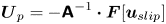 ${\boldsymbol U}_p = -\boldsymbol{\mathsf{A}}^{-1} \boldsymbol {\cdot } {\boldsymbol F}[{\boldsymbol {u}}_{slip}]$, where
  $\boldsymbol{\mathsf{A}}$ is the hydrodynamic resistance matrix of the particle and
  ${\boldsymbol F}[{\boldsymbol {u}}_{slip}]$ is the total force exerted across the surface
  $S$ as in (2.14). The methods described in previous sections can determine the relevant components of
  $\boldsymbol{\mathsf{A}}$ and
  ${\boldsymbol F}$ in an axisymmetric situation. Moreover, we can avoid the need to calculate slip velocity by using the identity (Lammert, Crespi & Nourhani Reference Lammert, Crespi and Nourhani2016)
 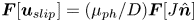 ${\boldsymbol F}[{\boldsymbol {u}}_{slip}] = ({\mu _{{ph}}}/{D}) {\boldsymbol F}[J\hat {\boldsymbol n}]$. Thus,
 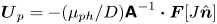 ${\boldsymbol U}_p = -({\mu _{{ph}}}/{D}) \boldsymbol{\mathsf{A}}^{-1} \boldsymbol {\cdot } {\boldsymbol F}[J\hat {\boldsymbol n}]$, where
  ${\boldsymbol F}[J\hat {\boldsymbol n}]$ is the total force resulting from velocity
  $J\hat {n}$ on the surface
  $S$. Finally, this last quantity can be calculated with the aid of the Lorentz reciprocal theorem. The result is the formula
 \begin{equation} {\boldsymbol U}_p ={-} \frac{\mu_{{ph}}}{D} \boldsymbol{\mathsf{A}}^{-1} \boldsymbol{\cdot} \boldsymbol{F}[\hat{\boldsymbol n}J] ={-}\frac{\mu_{{ph}} }{{D}} \int_S \boldsymbol{\mathsf{A}}^{-1}\boldsymbol{\cdot}\boldsymbol{\mathsf{E}}(\boldsymbol{r}_S)^{\rm T} \boldsymbol{\cdot} \hat{\boldsymbol n}J\, {\rm d} A, \end{equation}
for the self-propulsion velocity, where  $\boldsymbol{\mathsf{E}}$ is a rank-2 tensor closely related to the stress tensor induced by uniform velocity on
  $S$: For a passive particle moving at velocity
  ${\boldsymbol U}$, the hydrodynamic surface traction
  ${\boldsymbol f}_{\boldsymbol U}({ \boldsymbol r}_S) = \hat {\boldsymbol n}\boldsymbol {\cdot }\textsf{$\mathbf{\sigma}$}_{\boldsymbol U}({ \boldsymbol r}_S)$ is a linear function
  $\boldsymbol{\mathsf{E}}({ \boldsymbol r}_S)\boldsymbol {\cdot }{\boldsymbol U}$ of the velocity. This defines
  $\boldsymbol{\mathsf{E}}$; since
  ${\boldsymbol f}_{\boldsymbol U}({ \boldsymbol r}_S) = \hat {\boldsymbol n}\boldsymbol {\cdot }\textsf{$\mathbf{\sigma}$}_{\boldsymbol U}({ \boldsymbol r}_S), \boldsymbol{\mathsf{E}}$ can be calculated from the stress tensor. In fact, if the flux
  $J$ and the particle are axisymmetric,
  ${ \boldsymbol U}_p = {\mathcal {U}}_p \hat {\boldsymbol {e}}_{z}$ is along the symmetry axis, and
 \begin{equation} {\mathcal{U}}_p ={-}\frac{\mu_{{ph}} }{{D}} {A_{zz}}^{{-}1} \int_S \hat{\boldsymbol n} \boldsymbol{\cdot} \textsf{$\mathbf{\sigma}$}_{{\boldsymbol e}_z}({ \boldsymbol r}_S) \boldsymbol{\cdot} \hat{\boldsymbol n} \, J\, {\rm d} A, \end{equation}
where  $\textsf{$\mathbf{\sigma}$}_{{\boldsymbol e}_z}$ is the stress tensor associated with the surface velocity field
  ${ \boldsymbol {u}}_S = {\boldsymbol e}_z$.
We apply this to spheroids, with surface flux  $J$ in either a source/sink configuration, (uniform positive for
  $\eta > \eta _0$, uniform negative for
  $\eta < \eta _0$, with magnitudes such that net flux over the surface is zero), see figure 3, or a source/inert configuration, where the sink surface is replaced by an inert surface, in which case net flux is non-zero. The self-phoretic velocities for a range of eccentricity
  $\varepsilon$ and
  $\eta _0$, computed from (5.2) are plotted, scaled by the natural velocity scale
  ${\mathcal {U}}^{*} = \mu _{{ph}}\overline {|J|}/(2D)$, where overline indicates surface average. The results are in excellent agreement with exact solutions (Nourhani & Lammert Reference Nourhani and Lammert2016) for spheroids.

Figure 3. (a) Self-phoretic spheroid geometry:  $S''$ is source region,
  $S'$ sink or inert region. Here
  $\eta$ is a scaled
  $z$ coordinate;
  $a$ and
  $b$ are semi-axis lengths along and perpendicular to the symmetry axis;
 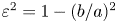 $\varepsilon ^{2} = 1-(b/a)^{2}$ is greater (less) than
  $1$ for prolate (oblate) spheroids. (b) Propulsion velocity for source/sink configuration, scaled to
  ${\mathcal {U}}^{*} \equiv \mu _{{ph}} \overline {|J|}/(2D)$. (c) Propulsion velocity for source/inert configuration.
6. Conclusion
We proposed a non-perturbative spectral method for low-Reynolds-number axisymmetric flow fields exterior to a radially deformed sphere. Implementation is simple, with no surface meshing, and the computational core being the solution of a set of linear algebraic equations. Still, it is well-suited to handle highly aspherical geometries. Our formalism for treating deformed spheres is built on Brenner's mapping (Brenner Reference Brenner1964a). The difference is that Brenner's method is perturbative and based on differential operations on the surface velocity field, whereas ours is non-perturbative and based on weighted integration of the boundary condition. It can perform well even in cases where perturbation theory may not work.
We have demonstrated the method on two problems. The first is hydrodynamic radii of spheres deformed in simple trigonometric patterns, albeit very strongly. The results were compared to BEM calculations, with good agreement. The second is a calculation of propulsion velocity of self-phoretic spheroids in the limit of the thin interfacial layer by a method which avoids computation of the slip velocity, although that could be handled as well. Axisymmetry occurs frequently in studies of microswimmers (Yariv Reference Yariv2011; Sabass & Seifert Reference Sabass and Seifert2012; Poehnl, Popescu & Uspal Reference Poehnl, Popescu and Uspal2020). Beyond spherical microswimmers (Nourhani et al. Reference Nourhani, Crespi and Lammert2015), a significant potential use of the formalism is to study the geometrical effects of high non-sphericity (Nourhani & Lammert Reference Nourhani and Lammert2016) on the dynamics of active particles and microswimmers and assist with advancing our understanding of the optimal geometry of slightly deformed spherical microswimmers (Daddi-Moussa-Ider et al. Reference Daddi-Moussa-Ider, Nasouri, Vilfan and Golestanian2021) to highly deformed ones. Moreover, the contribution of active particle shape to motion can then be consolidated in integration kernels (Nourhani & Lammert Reference Nourhani and Lammert2016) that quantify the contribution of local activity to swimmer dynamics. The current formalism can be advanced in multiple directions to include scenarios such as non-radial deformations, liquid droplets, deformed spheroids (to include deformed discotic and needle-like geometries), and extension to three-dimensional non-axisymmetric cases.
Acknowledgements
The authors are grateful to W. Uspal and V. Crespi for insightful comments and discussions.
Funding
This work is supported by funding from the University of Akron.
Declaration of interests
The authors report no conflict of interest.


 Open access