


1. Introduction
Several biological phenomena and industrial applications rely on separation and filtration processes such as the diffusion of water–glucose solutions through aquaporins (Jensen et al. Reference Jensen, Berg-Sørensen, Bruus, Holbrook, Liesche, Schulz, Zwieniecki and Bohr2016) and water purification (see Mohanty & Purkait Reference Mohanty and Purkait2011 for a review). Separation and filtration are often realized through the presence of thin permeable structures, i.e. membranes, which act as a discontinuity interface for the solvent and solute fields, and produce a thermodynamic imbalance between the two sides of the membrane (Bocquet & Palacci Reference Bocquet and Palacci2021). The tendency to compensate for this imbalance produces essential phenomena for biological processes (Bacchin, Glavatskiy & Gerbaud Reference Bacchin, Glavatskiy and Gerbaud2019). The imbalance is enhanced when Janus membranes are considered, i.e. functionalized thin porous surfaces with ‘contradictory’ (de Gennes Reference de Gennes1992; Zhao et al. Reference Zhao, Wang, Zhou and Lin2017) or asymmetric properties on the two opposite faces. These membranes show interesting opportunities to tackle energy-related challenges such as unidirectional oil/water separation, switchable ion transport, desalination and fog harvesting, to name a few (Yang et al. Reference Yang, Hou, Chen and Xu2016). Janus membranes have been investigated experimentally in the literature, and rely primarily on a common mechanism, i.e. the juxtaposition of lyophobic and lyophilic layers whose wettability contrast enables directional fluid transport from the first to the second layer, preventing flow in the opposite direction (Wang et al. Reference Wang, Ding, Dai, Wang and Lin2010; Wu et al. Reference Wu, Wang, Wang, Dong, Zhao and Jiang2012). The above-mentioned asymmetry can involve either geometrical and/or chemico-physical properties of the membrane surface corresponding to a different fabrication strategy (see Qian et al. Reference Qian2023 for a review). Membrane-based wound dressings with asymmetric properties are exploited to facilitate water evaporation, thus creating a dry environment, and promote hair follicle regeneration in burnt skin (de Groot et al. Reference de Groot, Ulrich, Gho and Huisman2021). Alternatively, by flipping the layers, it is possible to supply hydrogels to the epidermis for fast removal of necrotic tissues (An et al. Reference An2017). Other specific biomedical applications are related to the prevention of gastrointestinal retention (Lee et al. Reference Lee, Zhang, Lin, Langer and Traverso2016) or the reparation of tympanic membranes and other soft biological tissues (Liang et al. Reference Liang, He, Huang, Tang, Li, Zheng, Lin, Lu, Wang and Wu2022; Zhang et al. Reference Zhang, Li, Li, Zhu, Ren, Huang, Wu, Ji and Xu2022).
The specific modelling of Janus membranes is still in a germinal state and is based essentially on single-pore numerical simulations of the non-continuum molecular dynamics (Montes de Oca et al. Reference Montes de Oca, Dhanasekaran, Córdoba, Darling and de Pablo2022) or continuum models (Zhang et al. Reference Zhang, Sui, Li, Xie, Kong, Xiao, Gao, Wen and Jiang2017). Effective quantities such as the membrane permeability or conductivity, characterizing thick porous structures, are then retrieved heuristically from these simulations. The modelling of thick porous structures has been investigated deeply in the last century via formal multiscale techniques such as volume averaging and homogenization (cf. Whitaker (Reference Whitaker1996), Hornung (Reference Hornung1997), Mei & Vernescu (Reference Mei and Vernescu2010) and Davit et al. (Reference Davit2013) for a comparative review on the methods).
With regard to thin symmetric membranes, several simplified descriptions of the pure hydrodynamic problem have been proposed in the past. Hasimoto (Reference Hasimoto1958) and Wang (Reference Wang1994) focused on the pressure jump produced by a two-dimensional membrane formed by the repetition of slits or circular holes on a normal fluid flow. Tio & Sadhal (Reference Tio and Sadhal1994), starting from previous works of Beavers & Joseph (Reference Beavers and Joseph1967) and Saffman (Reference Saffman1971) on the interface conditions between a free fluid region and a bulk porous medium, quantified an averaged slip velocity in the vicinity of an infinitesimally thin porous screen. Jensen, Vincente & Stone (Reference Jensen, Vincente and Stone2014) unified the previous works of Sampson (Reference Sampson1891) and Weissberg (Reference Weissberg1962) to describe flows through membranes of arbitrary thickness with cylindrical holes. Bourgeat, Marusic & Marusic-Paloka (Reference Bourgeat, Marusic and Marusic-Paloka1997), Bourgeat, Gipouloux & Marusic-Paloka (Reference Bourgeat, Gipouloux and Marusic-Paloka2001) and Bourgeat & Marusic-Paloka (Reference Bourgeat and Marusic-Paloka1998) established a mathematical relation between the microscopic geometry of a thin membrane and the macroscopic permeability under strict macroscopic flow hypotheses. The above-mentioned works, related to the hydrodynamics of thin membranes, assume the continuity of the velocity field across the membrane. As concerns the flow of the solute–solvent couple through thin porous structures, only a few attempts to provide a theoretical proof of the heuristic Kedem–Katchalsky law, which describes the concentration jump across semipermeable membranes (Kedem & Katchalsky Reference Kedem and Katchalsky1958; Spiegler & Kedem Reference Spiegler and Kedem1966), have been made. Typically, authors considered specific pore geometries or specific far-field conditions for the unknown variables (Saffman Reference Saffman1960; Malone, Hutchinson & Prager Reference Malone, Hutchinson and Prager1974), thus showing limited predictive power. Kedem–Katchalsky-like models could be able to account for jumps in the unknown variables, but the general link between these jumps and the microscopic membrane properties is still missing (cf. Cardoso & Cartwright Reference Cardoso and Cartwright2014, for an attempt). Recently, a homogenization-based closed model to describe the flow of a dilute solution through a membrane was developed in Zampogna & Gallaire (Reference Zampogna and Gallaire2020) and Zampogna, Ledda & Gallaire (Reference Zampogna, Ledda and Gallaire2022). While these works do not show some of the limitations of the previous works on flows past thin membranes (e.g. in terms of applicability to generic microscopic or macroscopic membrane geometries or flow configuration) and establish a rigorous mathematical link between the microscopic and macroscopic membrane properties, the variables defining the state of the membrane system, i.e. the solvent velocity and solute concentration, are intrinsically continuous, making them unsuitable to describe the flow through Janus membranes, which is instead characterized by discontinuities in the concentration, pressure and velocity fields.
Here, we introduce a formal and robust approach to model discontinuities, and link them to the microscopic properties of Janus membranes, composed of the following essential steps: (i) problem formulation across the membrane; (ii) formal expression of the velocity, pressure and concentration fields as solutions of linear Stokes and Laplace microscopic problems, via the introduction of auxiliary variables not depending on the macroscopic outer flow (§ 2.1); (iii) upscaling of the microscopic solution to the macroscopic level through an averaging procedure (§§ 2.2 and 2.3). The paper is organized as follows. Section 2 presents the equations governing the motion of the couple solute–solvent in the vicinity of the membrane pores, and the development of the equivalent macroscopic model to enable jumps in the – previously continuous – unknown variables. In § 3, we relate the above-mentioned auxiliary variables to the physical properties of the membrane, such as permeability, slip and solute diffusivity, and quantify them via the new model through the solution of several microscopic problems. Section 4 compares the macroscopic model with the solution of the full-scale equations where the microstructure, together with its thermodynamic properties, is fully represented. Finally, in § 5, we discuss the perspectives opened in the modelling of membrane flows.
2. Macroscopic model for mass transport through thin membranes
Let us consider a solute of molecular diffusivity  $D$ transported by the flow of an incompressible Newtonian fluid, the solvent, of constant density $\rho$ and viscosity $\mu$. We neglect variations of the solvent properties due to the concentration of the solute. The solution flows through a microstructured membrane of characteristic size $L$, composed by a periodic repetition of solid inclusions whose typical size is $l$ (cf. figure 1). Owing to the multiscale nature of the membrane, the relation between $l$ and $L$ defines the separation of scales parameter $\epsilon$ such that $\epsilon =l/L\ll 1$. The flow equations for the concentration, velocity and pressure fields ( $c, u_i, p$) are non-dimensionalized with a characteristic far-field velocity $U$, concentration difference $\Delta C$, viscous stress $\mu U /L$, macroscopic membrane size $L$, and characteristic time $T=L/U$:
 \begin{equation} \partial_{i}u_i=0, \quad {Re}\left(\partial_t u_i+u_j\,\partial_ju_i\right)=\partial_j\varSigma_{ij} , \quad {Pe}\,\partial_t c=\partial_jF_j , \end{equation}
where  $i,j=1,2,3$ (cf. figure 1a), $\varSigma _{ij}=-p\delta _{ij}+(\partial _{j}u_i+\partial _{i}u_j)$ is the fluid stress tensor, $F_j=-{Pe}\,u_jc+\partial _{j}c$ is the solute flux, ${Pe}=U L/D$ and ${Re}=\rho U L/\mu$ are the Péclet and Reynolds numbers, and $\delta _{ij}$ is the Kronecker delta. Generic boundary conditions for $u_i$ and $c$ are imposed on the membrane solid walls $\partial \mathbb {M}$ (cf. figure 1):
 \begin{equation} \alpha_i(\boldsymbol{x})\,\varSigma_{ij}\,\alpha'_j(\boldsymbol{x})=\beta_i(\boldsymbol{x})\,u_i-\gamma_i(\boldsymbol{x})\,U_i^{\partial\mathbb{M}}, \quad \zeta_i(\boldsymbol{x})\,F_i=\eta(\boldsymbol{x})\,\kappa c-\lambda(\boldsymbol{x})\,\kappa C^{\partial\mathbb{M}}. \end{equation}
The parameters  $\alpha _i, \alpha '_i,\beta _i,\gamma _i,\zeta _i,\eta,\lambda$ are defined on $\partial \mathbb {M}$ and allow us to describe several membrane behaviours. Quantities $U_i^{\partial \mathbb {M}}$ and $C^{\partial \mathbb {M}}$ instead denote the values of velocity and concentration when a Dirichlet boundary condition is imposed at the membrane. Among the several combinations of the space-dependent parameters $\alpha _i, \alpha '_i,\beta _i,\gamma _i,\zeta _i,\eta, \lambda$, we mention those that are physically most natural. Introducing the tangential $t_i, s_i$ and normal $n_i$ vectors associated with $\partial \mathbb {M}$, when $\alpha _i=t_i$, $\alpha '_i=\beta _i=n_i$ and $\gamma _i=0$, zero-shear and no-penetration are imposed on $\partial \mathbb {M}$, which is likely to have a hydrophobic behaviour. Inversely, the no-slip boundary condition, namely a hydrophilic solvent–membrane interaction, is realized by choosing $\alpha _i=\alpha '_i=\gamma _i=0$ and $\beta _i=1$. The several types of solute–membrane interactions that can be realized by varying the values of $\zeta _i$, $\eta$ and $\lambda$ have been analysed in Zampogna et al. (Reference Zampogna, Ledda and Gallaire2022); the membrane has a chemostat-like behaviour when $\zeta _i=0$ and $\eta =\lambda =1$, an insulating behaviour when $\zeta _i=n_i$ and $\eta =\lambda =0$, and an absorbing/desorbing behaviour for $\zeta _i=n_i$, $\eta =\pm 1$ and $\lambda =0$.

Figure 1. Sketches of a microstructured membrane. (a) Full-scale sketch of the membrane invested by a fluid flow that carries a diluted solute. The membrane is asymmetric with respect to its central surface since it is formed by a net of triangular prisms. (b) Periodic unitary elementary cell of the membrane. (c) Equivalent homogenized macroscopic membrane where conditions (2.15) are imposed.
In the case of  ${Re}$ and ${Pe}$ up to ${O}(\epsilon ^{-1})$, i.e. when the pore Reynolds and Péclet numbers $Re^{\mathbb {I}}=\rho U^{\mathbb {I}} l/\mu =\epsilon ^2\,Re$ and $Pe^{\mathbb {I}}=U^{\mathbb {I}} l/D=\epsilon ^2\,Pe$, based on the typical pore size and velocity, $l$ and $U^{\mathbb {I}}$, are up to ${O}(\epsilon )$, the solution of (2.1a–c) and (2.2a,b) in the whole full-scale domain converges, on average, to the solution of the problem where the membrane is replaced by a smooth macroscopic interface $\mathbb {C}$ between two fluid regions where (2.1a–c) still apply; see figure 1 (Zampogna & Gallaire Reference Zampogna and Gallaire2020; Ledda et al. Reference Ledda, Boujo, Camarri, Gallaire and Zampogna2021; Zampogna et al. Reference Zampogna, Ledda and Gallaire2022). The macroscopic interface conditions imposed on $\mathbb {C}$ stem from the application of homogenization to (2.1a–c) and (2.2a,b). The main steps of the procedure are recalled in the next section.
2.1. Homogenization of the governing equations
To develop the macroscopic interface conditions valid on  $\mathbb {C}$, the procedure initially developed in Zampogna & Gallaire (Reference Zampogna and Gallaire2020) focuses on the solution of the problem within the microscopic domain sketched in figure 1(b). The full-scale spatial variable $x_i$ is decomposed as $x_i\rightarrow x_i'+x_i$, with $x_i'=x_i/\epsilon$, so that $x_i\rightarrow 0^\pm$ when $x'_i\rightarrow \pm \infty$, and vice versa. We denote as $x_i'$ the microscopic variable defined within the microscopic elementary cell, also called the inner domain, while $x_i$ is the macroscopic variable defined outside the microscopic elementary cell, the outer domain. We employ a local reference frame $(t,s,n)$, where $(t,s)$ and $n$ are the local tangential and normal directions to the membrane, respectively. To close (2.1a–c) and (2.2a,b) on the microscopic domain, flow periodicity is imposed along $x'_t$ and $x'_s$, while the continuity of velocities, concentration, solvent tractions and solute normal fluxes are exploited over $\mathbb {U}$ and $\mathbb {D}$. We decompose the unknown variables in (2.1a–c) with the multiple scale expansions $(c,p)=\sum _{n=0}^{N}\epsilon ^n(c^{(n)},p^{(n)})$ and $u_i=\sum _{n=0}^{N}\epsilon ^{n+1}u_i^{(n)}$. After substituting these expansions in (2.1a–c) and (2.2a,b), and collecting the leading-order terms in the separation of scales parameter $\epsilon$ (Hornung Reference Hornung1997), we obtain
 \begin{equation} 0={-}\partial_ip^{(0)}+\partial_{ii}^2u_i^{(0)}, \quad 0=\partial_iu^{(0)},\quad 0=\partial_{ii}^2c^{(0)}. \end{equation}
Following Zampogna & Gallaire (Reference Zampogna and Gallaire2020) and Zampogna et al. (Reference Zampogna, Ledda and Gallaire2022), the microscopic solution of (2.3a–c) can be written as a linear combination of the outer fluid stresses and solute fluxes that enter the microscopic problems in the boundary conditions on the sides  $\mathbb {U}$ and $\mathbb {D}$ of the microscopic elementary cell (cf. figure 1b), i.e.
 \begin{gather} {u_i}=\epsilon\left({M}_{ijk}\varSigma_{jk}\vert_{\mathbb{C^-}}+{N}_{ijk}\varSigma_{jk}\vert_{\mathbb{C^+}}\right), \end{gather}
 \begin{gather} {p}={Q}_{jk}\varSigma_{jk}\vert_{\mathbb{C^-}}+{R}_{jk}\varSigma_{jk}\vert_{\mathbb{C^+}}, \end{gather}
 \begin{gather} {c}=C_0+\epsilon \left({T}_{i}F_{i}\vert_{\mathbb{C^-}}+{Y}_{i}F_{i}\vert_{\mathbb{C^+}}\right), \end{gather}
where the superscript  $^{(0)}$ has been omitted for ease of notation, and the notations $\vert _{\mathbb {C}^\pm }$ denote solvent stresses $\varSigma _{jk}$ and solute fluxes $F_i$ calculated on the upward and downward sides of the macroscopic membrane $\mathbb {C}$, as depicted in figure 1(c). The quantity indicated with $C_0$ in (2.6) represents a mean base value for $c$, which can be retrieved by an integral balance of the solute governing equations on a control volume equal to the microscopic elementary cell identified in figure 1(b). (cf. Zampogna et al. Reference Zampogna, Ledda and Gallaire2022). We refer to Appendix A for further insights on how to calculate $C_0$.
Quantities  $M_{ijk}$, $N_{ijk}$, $Q_{jk}$, $R_{jk}$, $T_i$ and $Y_i$ are defined over the microscopic domain sketched in figure 1(b). Substituting (2.10)–(2.12) into (2.3a–c), the partial differential equations satisfied by these coefficients in the fluid part $\mathbb {F}$ of the microscopic elementary cell are found:
 \begin{equation} \left.\begin{aligned}
&-\partial_i Q_{jk}+\partial^2_{ll} M_{ijk}=0,
\quad\text{in }\mathbb{F}, \\ &\partial_i
M_{ijk}=0, \quad\text{in }\mathbb{F},\\
&\alpha\,\partial_nM_{ijk}=\beta M_{ijk},\quad \text{on
}\partial\mathbb{M},\\ &\varSigma_{pq}(M_{{\cdot} jk},
Q_{jk})\,n_q=\delta_{jp}\delta_{kq}n_q,\quad \text{on
}\mathbb{U}, \\ &\varSigma_{pq}(M_{{\cdot} jk},
Q_{jk})\,n_q=0, \quad \text{on }\mathbb{D},
\end{aligned}\right\}\quad \left.\begin{aligned}
&{-\partial_i}R_{jk}+\partial^2_{ll} N_{ijk}=0,
\quad\text{in }\mathbb{F}, \\ &\partial_i N_{ijk}=0,
\quad\text{in }\mathbb{F},\\
&\alpha\,\partial_nN_{ijk}=\beta N_{ijk}, \quad \text{on
}\partial\mathbb{M},\\ &\varSigma_{pq}(N_{{\cdot} jk},
R_{jk})\,n_q=0, \quad \text{on }\mathbb{U},\\
&\varSigma_{pq}(N_{{\cdot} jk},
R_{jk})\,n_q=\delta_{jp}\delta_{kq}n_q,\quad \text{on
}\mathbb{D}, \end{aligned} \right\}
\end{equation}
\begin{equation} \left.\begin{aligned}
&-\partial_i Q_{jk}+\partial^2_{ll} M_{ijk}=0,
\quad\text{in }\mathbb{F}, \\ &\partial_i
M_{ijk}=0, \quad\text{in }\mathbb{F},\\
&\alpha\,\partial_nM_{ijk}=\beta M_{ijk},\quad \text{on
}\partial\mathbb{M},\\ &\varSigma_{pq}(M_{{\cdot} jk},
Q_{jk})\,n_q=\delta_{jp}\delta_{kq}n_q,\quad \text{on
}\mathbb{U}, \\ &\varSigma_{pq}(M_{{\cdot} jk},
Q_{jk})\,n_q=0, \quad \text{on }\mathbb{D},
\end{aligned}\right\}\quad \left.\begin{aligned}
&{-\partial_i}R_{jk}+\partial^2_{ll} N_{ijk}=0,
\quad\text{in }\mathbb{F}, \\ &\partial_i N_{ijk}=0,
\quad\text{in }\mathbb{F},\\
&\alpha\,\partial_nN_{ijk}=\beta N_{ijk}, \quad \text{on
}\partial\mathbb{M},\\ &\varSigma_{pq}(N_{{\cdot} jk},
R_{jk})\,n_q=0, \quad \text{on }\mathbb{U},\\
&\varSigma_{pq}(N_{{\cdot} jk},
R_{jk})\,n_q=\delta_{jp}\delta_{kq}n_q,\quad \text{on
}\mathbb{D}, \end{aligned} \right\}
\end{equation} \begin{equation} \left.\begin{aligned}
&\partial_{ii}^2T_j=0, \quad \text{in } \mathbb{F}, \\
&\zeta\,\partial_iT_jn_i=\lambda T_j, \quad \text{on }
\partial\mathbb{M},\\ &\partial_iT_jn_i=n_j, \quad \text{on
} \mathbb{U}, \\ &\zeta T_j=\lambda\,\partial_iT_jn_i,\quad
\text{on } \mathbb{D}, \end{aligned} \right\} \quad
\left. \begin{aligned} & \partial_{ii}^2Y_j=0 ,\quad \text{in }
\mathbb{F}, \\ &\zeta\,\partial_iY_jn_i=\lambda Y_j, \quad
\text{on } \partial\mathbb{M},\\ &\zeta
Y_j=\lambda\,\partial_i Y_jn_i,\quad \text{on } \mathbb{U},
\\ &\partial_iY_jn_i=n_j, \quad \text{on } \mathbb{D},
\end{aligned} \right\}
\end{equation}
\begin{equation} \left.\begin{aligned}
&\partial_{ii}^2T_j=0, \quad \text{in } \mathbb{F}, \\
&\zeta\,\partial_iT_jn_i=\lambda T_j, \quad \text{on }
\partial\mathbb{M},\\ &\partial_iT_jn_i=n_j, \quad \text{on
} \mathbb{U}, \\ &\zeta T_j=\lambda\,\partial_iT_jn_i,\quad
\text{on } \mathbb{D}, \end{aligned} \right\} \quad
\left. \begin{aligned} & \partial_{ii}^2Y_j=0 ,\quad \text{in }
\mathbb{F}, \\ &\zeta\,\partial_iY_jn_i=\lambda Y_j, \quad
\text{on } \partial\mathbb{M},\\ &\zeta
Y_j=\lambda\,\partial_i Y_jn_i,\quad \text{on } \mathbb{U},
\\ &\partial_iY_jn_i=n_j, \quad \text{on } \mathbb{D},
\end{aligned} \right\}
\end{equation}
where  $i,j,k,l=t,s,n$. Periodicity along the tangent to the membrane directions $x_s'$ and $x_t'$ is imposed. The Stokes and Laplace problems (2.7) and (2.8) represent the solvability conditions of solutions (2.4)–(2.6). From a mathematical point of view, the components of the tensors and vectors in (2.4)–(2.6) are the coefficients of the linear combination relating the velocity and pressure fields to the fluid stresses and the concentration field to the solute fluxes. We will clarify their physical meaning after the upscaling of conditions (2.4)–(2.6).
2.2. Upscaling the microscopic solution with central average
To upscale (2.4)–(2.6), Zampogna & Gallaire (Reference Zampogna and Gallaire2020) and Zampogna et al. (Reference Zampogna, Ledda and Gallaire2022) introduced the central average within the microscopic elementary cell, defined as
 \begin{equation} \bar{\cdot}=\lim_{x_n'\rightarrow0^{{\pm}}}\frac{1}{|\mathbb{C}_{\mathbb{F}}\cup\mathbb{C}_{\mathbb{M}}|}\int_{\mathbb{C}_{\mathbb{F}}}\,\mathrm{d}\kern 0.06em x_s'\,\mathrm{d}\kern 0.06em x_t', \end{equation}
where  $\mathbb {C}_{\mathbb {F}}$ and $\mathbb {C}_{\mathbb {M}}$ denote the fluid and solid regions on $\mathbb {C}$. The average defined in (2.9), i.e. the integral on the projection of $\mathbb {C}$ within the microscopic elementary cell (blue plane in figure 1b), renders the unknown solvent velocity and solute concentration fields continuous across the macroscopic interface $\mathbb {C}$. The macroscopic interface conditions valid on the homogeneous, macroscopic domain $\mathbb {C}$ (cf. figure 1c) are retrieved by applying average (2.9) to (2.4)–(2.6):
 \begin{gather} u_i\vert_{\mathbb{C}}=u_i\vert_{\mathbb{C}^-}=u_i\vert_{\mathbb{C}^+}=\overline{u_i}=\epsilon\left(\bar{M}_{ijk}\varSigma_{jk}\vert_{\mathbb{C^-}}+\bar{N}_{ijk}\varSigma_{jk}\vert_{\mathbb{C^+}}\right), \end{gather}
 \begin{gather} p\vert_{\mathbb{C}}=\bar{p}=\bar{Q}_{jk}\varSigma_{jk}\vert_{\mathbb{C^-}}+\bar{R}_{jk}\varSigma_{jk}\vert_{\mathbb{C^+}}, \end{gather}
 \begin{gather} c\vert_{\mathbb{C}}=c\vert_{\mathbb{C}^-}=c\vert_{\mathbb{C}^+}=\bar{c}=C_0+\epsilon \left(\bar{T}_{i}F_{i}\vert_{\mathbb{C^-}}+\bar{Y}_{i}F_{i}\vert_{\mathbb{C^+}}\right). \end{gather}
Equations (2.10)–(2.12) quantify the values of the unknown fields at the membrane global size and transfer the global effects of the presence of the inclusions from a microscopic to a macroscopic scale. Tensors  $M_{ijk}$ and $N_{ijk}$ are labelled as upward and downward Navier tensors, which provide information about the mobility of the fluid in the vicinity of the macroscopic membrane $\mathbb {C}$. In local curvilinear coordinates, on the plane $(x'_n,x'_t)$, $\bar {M}_{nnn}$ and $\bar {M}_{ntn}$ represent the ability of the fluid to flow along the normal direction, while $\bar {M}_{tnn}$ and $\bar {M}_{ttn}$ represent the ability of the fluid to flow along the tangential direction. Here, $\bar {N}_{ijk}$ has the same physical meaning of $\bar {M}_{ijk}$ when the downward side of the membrane is considered, instead of the upward one. In the frame of reference of the membrane, only tensor components whose third index is equal to $n$ are different from zero, since the source terms in the linear microscopic problems come from the continuity of fluid tractions $\varSigma ^+_{ij}n_j$ on $\mathbb {U}$ and $\mathbb {D}$. As shown in Ledda et al. (Reference Ledda, Boujo, Camarri, Gallaire and Zampogna2021), one could define two second-order tensors, $M'_{ij}=\bar {M}_{ijn}$ and $N'_{ij}=\bar {N}_{ijn}$, which contain the same information about the corresponding third-order tensors, and can be linked to the classical second-order permeability tensor that characterizes traditional bulk porous structures. The reader is referred to Zampogna & Gallaire (Reference Zampogna and Gallaire2020) for a comparison between the homogenized solution and the analytical pressure drop across a porous screen made of circular holes (Jensen et al. Reference Jensen, Vincente and Stone2014).
The quantities  $\bar {Q}_{jk}$ and $\bar {R}_{jk}$ are auxiliary variables introduced to relate formally the leading-order pressure to the outer fluid stresses. As noticed in Zampogna & Gallaire (Reference Zampogna and Gallaire2020), (2.11) does not contribute to the determination of the leading-order solution since a macroscopic pressure jump is produced across the membrane, and the value of the jump is set by the normal component of (2.10) that contains $p\vert _{\mathbb {C^{\pm }}}$.
As will be shown in § 4.2, (2.11) allows one to a posteriori retrieve the value of pressure at the centre of the membrane  $\mathbb {C}$, and then has little physical utility. Vectors $\bar {T}_i$ and $\bar {Y}_i$ can be defined as upward and downward effective diffusivities, and quantify the variations of the solute diffusivity due to the presence of the solid microstructure.
The macroscopic model (2.10)–(2.12) is obtained by applying the central average (2.9) to the solution (2.4)–(2.6) of the leading-order governing equations (2.3a–c). The central average approach provides a good estimation of the full-scale flow fields when the membrane properties exhibit slow and small variations in the filtration direction along each single pore (Zampogna & Gallaire Reference Zampogna and Gallaire2020). When the variations are fast and large, the central average approach may oversimplify the far-field effects produced by the strong gradients across the pores. When an imbalance between the upward and downward sides of such a porous screen is considered, e.g. with free-slip on one side and no-slip on the other, exotic effects may occur, with different tangential velocities on each side, which are not properly described by a central average model. Since the velocity and concentration fields are continuous across the membrane, macroscopic boundary conditions symmetric with respect to  $\mathbb {C}$ can produce only symmetric flow fields. As suggested previously, in the case of Janus membranes, while full-scale flow fields are continuous, discontinuities may emerge in the macroscopic, averaged fields, from imbalance effects due to asymmetric properties of the microscopic membrane geometry. In the next subsection, we will present a modified average (2.9) that accounts for discontinuities in the upscaled fields.
2.3. Introducing macroscopic flow field discontinuities
The spatial average (2.9) plays a crucial role in the continuity of the flow fields. A different spatial average is introduced to allow discontinuous quantities on each side of the membrane. In Zampogna & Gallaire (Reference Zampogna and Gallaire2020) and Zampogna et al. (Reference Zampogna, Ledda and Gallaire2022), the matching between the microscopic and macroscopic generic field  $f$ is expressed via the limit
 \begin{equation} \lim_{x_n'\rightarrow\pm\infty}f(x_n')=\lim_{x_n\rightarrow0^{{\pm}}}f(x_n). \end{equation}
We define two different averages computed in the positive and negative microscopic far field:
 \begin{equation}
\bar{\cdot}^{^-}=\lim_{x_n'\rightarrow+\infty}\frac{1}{|\mathbb{U}|}\int_{\mathbb{U}}\,\mathrm{d}\kern
0.06em x_s'\,\mathrm{d}\kern 0.06em x_t'
\quad\text{and}\quad\bar{\cdot}^{^+}=\lim_{x_n'\rightarrow-\infty}\frac{1}{|\mathbb{D}|}\int_{\mathbb{D}}\,\mathrm{d}\kern
0.06em x_s'\,\mathrm{d}\kern 0.06em x_t',
\end{equation}
\begin{equation}
\bar{\cdot}^{^-}=\lim_{x_n'\rightarrow+\infty}\frac{1}{|\mathbb{U}|}\int_{\mathbb{U}}\,\mathrm{d}\kern
0.06em x_s'\,\mathrm{d}\kern 0.06em x_t'
\quad\text{and}\quad\bar{\cdot}^{^+}=\lim_{x_n'\rightarrow-\infty}\frac{1}{|\mathbb{D}|}\int_{\mathbb{D}}\,\mathrm{d}\kern
0.06em x_s'\,\mathrm{d}\kern 0.06em x_t',
\end{equation}
called respectively upward and downward averages. Applying the new averages to the solution of the leading-order governing equations (2.3a–c) in the microscopic elementary cell, the following conditions for the velocity, concentration and pressure fields on the sides of the membrane  $\mathbb {C}^{\pm }$ are obtained:
 \begin{equation} \left. \begin{aligned}
\overline{u_i}^{^-}=\epsilon\left(\mathcal{M}_{ijk}^{-}\varSigma_{jk}\vert_{\mathbb{C^-}}+\mathcal{N}_{ijk}^{-}\varSigma_{jk}\vert_{\mathbb{C^+}}\right),\\
\overline{u_i}^{^+}=\epsilon\left(\mathcal{M}_{ijk}^+\varSigma_{jk}\vert_{\mathbb{C^-}}+\mathcal{N}_{ijk}^+\varSigma_{jk}\vert_{\mathbb{C^+}}\right),
\end{aligned} \right\} \quad \left. \begin{aligned}
\bar{c}^{^-}=C_0+\epsilon
\left(\mathcal{T}_i^{-}F_{i}\vert_{\mathbb{C^-}}+\mathcal{Y}_{i}^{-}F_{i}\vert_{\mathbb{C^+}}\right),\\
\bar{c}^{^+}=C_0+\epsilon
\left(\mathcal{T}_{i}^+F_{i}\vert_{\mathbb{C^-}}+\mathcal{Y}_i^+F_{i}\vert_{\mathbb{C^+}}\right),
\end{aligned} \right\}
\end{equation}
\begin{equation} \left. \begin{aligned}
\overline{u_i}^{^-}=\epsilon\left(\mathcal{M}_{ijk}^{-}\varSigma_{jk}\vert_{\mathbb{C^-}}+\mathcal{N}_{ijk}^{-}\varSigma_{jk}\vert_{\mathbb{C^+}}\right),\\
\overline{u_i}^{^+}=\epsilon\left(\mathcal{M}_{ijk}^+\varSigma_{jk}\vert_{\mathbb{C^-}}+\mathcal{N}_{ijk}^+\varSigma_{jk}\vert_{\mathbb{C^+}}\right),
\end{aligned} \right\} \quad \left. \begin{aligned}
\bar{c}^{^-}=C_0+\epsilon
\left(\mathcal{T}_i^{-}F_{i}\vert_{\mathbb{C^-}}+\mathcal{Y}_{i}^{-}F_{i}\vert_{\mathbb{C^+}}\right),\\
\bar{c}^{^+}=C_0+\epsilon
\left(\mathcal{T}_{i}^+F_{i}\vert_{\mathbb{C^-}}+\mathcal{Y}_i^+F_{i}\vert_{\mathbb{C^+}}\right),
\end{aligned} \right\}
\end{equation} \begin{equation} {\begin{aligned}
\bar{p}^{^-}=\mathcal{Q}_{jk}^{-}\varSigma_{jk}\vert_{\mathbb{C^-}}+\mathcal{R}_{jk}^{-}\varSigma_{jk}\vert_{\mathbb{C^+}},\\
\bar{p}^{^+}=\mathcal{Q}_{jk}^+\varSigma_{jk}\vert_{\mathbb{C^-}}+\mathcal{R}_{jk}^+\varSigma_{jk}\vert_{\mathbb{C^+}},
\end{aligned}}
\end{equation}
\begin{equation} {\begin{aligned}
\bar{p}^{^-}=\mathcal{Q}_{jk}^{-}\varSigma_{jk}\vert_{\mathbb{C^-}}+\mathcal{R}_{jk}^{-}\varSigma_{jk}\vert_{\mathbb{C^+}},\\
\bar{p}^{^+}=\mathcal{Q}_{jk}^+\varSigma_{jk}\vert_{\mathbb{C^-}}+\mathcal{R}_{jk}^+\varSigma_{jk}\vert_{\mathbb{C^+}},
\end{aligned}}
\end{equation}with
 \begin{equation} \left. \begin{gathered} \mathcal{M}_{ijk}^{-}=\bar{M}_{ijk}^{^-}-x_n\vert_{\mathbb{U}}(\delta_{it}\delta_{jt}+\delta_{is}\delta_{js})\delta_{kn}, \quad \mathcal{M}_{ijk}^+ = \bar{M}_{ijk}^{^+}, \quad {\mathcal{Q}^\pm_{ij}=\bar{Q}^\pm_{ij},}\\ \mathcal{T}_i^{-}=\bar{T}_{i}^{^-}-x_n\vert_{\mathbb{U}}\delta_{in},\quad \mathcal{T}_i^+ = \bar{T}_i^{^+},\\ \mathcal{N}_{ijk}^{-}=\bar{N}_{ijk}^{^-}, \quad \mathcal{N}_{ijk}^+ = \bar{N}_{ijk}^{^+}-x_n\vert_{\mathbb{D}}(\delta_{it}\delta_{jt}+\delta_{is}\delta_{js})\delta_{kn},\quad {\mathcal{R}^\pm_{ij}=\bar{R}^\pm_{ij},}\\ \mathcal{Y}_i^{-}=\bar{Y}_i^{^-},\quad \mathcal{Y}_i^+ = \bar{Y}_{i}^{^+}-x_n\vert_{\mathbb{D}}\delta_{in}. \end{gathered} \right\} \end{equation}
Equations (2.15) and (2.16) are the set of interface conditions that quantify the solute–solvent flow at the Janus membranes. The interface conditions (2.15) transfer the asymmetry of the membrane from the microscopic level to the macroscopic one, inducing asymmetric flow fields even when the macroscopic flow configuration is symmetric with respect to  $\mathbb {C}$. The jump in the macroscopic velocity and concentration fields between the upward and downward sides of the membrane is given by the difference between the upward and downward averages of the microscopic tensors $M_{ijk}$ and $N_{ijk}$ for the velocity, and the vectors $T_{i}$ and $Y_{i}$ for the concentration. These microscopic quantities stem from the nature of the Janus membrane, which produces asymmetric interactions between the membrane and the surrounding fluid, at a microscopic level. The upward (resp. downward) averaged tensors $\mathcal {M}_{ijk}^{-}$ (resp. $\mathcal {M}_{ijk}^+$) and $\mathcal {N}_{ijk}^{-}$ (resp. $\mathcal {N}_{ijk}^+$) estimate the effect of the membrane on the upward (resp. downward) flow due to an upward and downward stress. Similarly, the upward (resp. downward) averaged vectors $\mathcal {T}_i^{-}$ (resp. $\mathcal {T}_i^+$) and $\mathcal {Y}_i^{-}$ (resp. $\mathcal {Y}_i^+$) measure variations of the upward (resp. downward) solute concentration from $C_0$ due to the effects of the upward and downward diffusive fluxes. The new model (2.15) remains a leading-order approximation of the full-scale solution but provides an enriched flow description with respect to its continuous counterpart (2.10)–(2.12), and better suits an extended set of thin porous membranes, whose properties along the filtration direction may exhibit important variations. The number of effective parameters describing the macroscopic flow, doubled with respect to the previous case, reflects this richness.
As concerns  $\mathcal {Q}^\pm _{ij}$ and $\mathcal {R}^{\pm }_{ij}$, Zampogna & Gallaire (Reference Zampogna and Gallaire2020) showed in the central average case that only the fields $Q_{nn}$ and $R_{nn}$ can play a role in the macroscopic solution since the other components are antisymmetric with respect to the planes $x'_t=0$ and $x'_s=0$, or identically zero as solutions of homogeneous problems. The far-field boundary conditions on $\mathbb {U}$ and $\mathbb {D}$ in the microscopic problems (2.7) read
 \begin{equation} \left. \begin{aligned} &
Q_{nn}=1, \quad \text{on } \mathbb{U},\\ & Q_{nn}=0, \quad
\text{on }\mathbb{D}, \end{aligned} \right\} \quad
\left. \begin{aligned} & R_{nn}=0, \quad \text{on } \mathbb{U},\\
& R_{nn}=1, \quad \text{on }\mathbb{D}, \end{aligned} \right\}
\end{equation}
\begin{equation} \left. \begin{aligned} &
Q_{nn}=1, \quad \text{on } \mathbb{U},\\ & Q_{nn}=0, \quad
\text{on }\mathbb{D}, \end{aligned} \right\} \quad
\left. \begin{aligned} & R_{nn}=0, \quad \text{on } \mathbb{U},\\
& R_{nn}=1, \quad \text{on }\mathbb{D}, \end{aligned} \right\}
\end{equation}
since the viscous contribution of the stress is negligible far from the solid inclusion on  $\mathbb {U}$ and $\mathbb {D}$. After substituting these values in (2.16), one retrieves the trivial identities $\bar {p}^\pm =p\vert _{\mathbb {C}^{\pm }}$. As for the central average case, (2.16) does not contribute to the leading-order flow approximation. The interface conditions (2.15) rely on the knowledge of the microscopic fields $M_{ijk}$, $N_{ijk}$, $T_{i}$ and $Y_{i}$, which will be analysed in the next section.
3. Effects of the new averages on the microscopic problems
In the previous section, we have shown that  $\mathcal {Q}^\pm _{ij}$ and $\mathcal {R}^\pm _{ij}$ do not contribute to the determination of the macroscopic flow at the membrane $\mathbb {C}$, and do not deserve any further microscopic analysis. Conversely, the quantities $M_{ijk}$, $N_{ijk}$, $T_{i}$ and $Y_{i}$ have been analysed thoroughly in Zampogna & Gallaire (Reference Zampogna and Gallaire2020) and Zampogna et al. (Reference Zampogna, Ledda and Gallaire2022). Here, we show the modifications of the effective, macroscopic values induced by the upward and downward averages. Equations (2.7) and (2.8) are solved numerically within the microscopic domains sketched in figure 2 using their weak form implementation in the finite-element solver COMSOL Multiphysics. The spatial discretization is based on the Taylor–Hood (P2-P1) triangular elements for the solvent tensors, and P3 triangular elements for the solute vectors. We use mesh spacing $\Delta l_1=0.01$ at the boundaries of the microscopic cell, and we guarantee at least $25$ grid points on each side of the solid inclusions when the spacing $\Delta l_1$ produces less than 25 points on that side. Other simulations have been carried out on coarser meshes with spacing $\Delta l_2=0.02$ and $\Delta l_3=0.04$, and numerical convergence of the average value of $T_n$ up to $0.1\,\%$ has been verified between $\Delta l_1$ and $\Delta l_2$.

Figure 2. Considered microscopic inclusions and boundary conditions for the solvent and solute fields. Inclusions  $G1$ and $GF1$ are equilateral triangles with height $0.5l$, equal to the side of the square inclusion considered in $F1$.
$F1$.
Three different types of asymmetries are considered, denoted in figure 2 as  $G1$ (purely geometrical), $F1$ (purely functional) and $GF1$ (functional and geometrical). In $G1$, the no-slip condition for $u_i$ and a chemostat-like condition $c=0$ are imposed everywhere on $\partial \mathbb {M}$. In $F1$ and $GF1$, instead, the upstream region (highlighted in yellow) is a hydrophilic-like surface, $u_i=0$, while the downstream region (highlighted in purple) is an idealized hydrophobic surface with zero wall-normal solvent stress. For the concentration field, a chemostat-like condition $c=0$ is imposed on the upstream region, while the downstream region is made by an insulating material, $\partial _ic\,n_i=0$.
3.1. Effect of the asymmetry on the averaged microscopic quantities
Before proceeding with a thorough analysis of the microscopic solution associated with the different types of solid inclusions mentioned in the previous section, we provide some intuition about the effects of asymmetry on the new averaged microscopic quantities. The upward and downward averages should produce different values of the effective tensors only when membrane properties are not symmetric with respect to the centreline of the membrane  $\mathbb {C}$. To confirm this feature and show the continuous transition from symmetric to asymmetric membrane properties, we report in figure 3 the values of $\mathcal {M}^-_{ttn}$, $\mathcal {N}^+_{ttn}$, $\mathcal {T}^-_n$ and $\mathcal {Y}^+_n$. We consider a square inclusion of perimeter $\sigma =1$ with no-slip and zero solute concentration imposed on $\partial \mathbb {M}$. We then introduce a microscopic functional asymmetry by imposing zero-shear, no-penetration and insulating conditions on the green portion of $\partial \mathbb {M}$ whose length $\Delta \sigma$ is increased smoothly from 0 to $\sigma$. When the functional asymmetry on the membrane is not present, i.e. for $\Delta \sigma =0$ or $\Delta \sigma =1$, the upward and downward averages of $\mathcal {M}^-_{ttn}$, $\mathcal {N}^+_{ttn}$, $\mathcal {T}^-_n$ and $\mathcal {Y}^+_n$ have same values. For the other values of $\Delta \sigma$, differences between these values are noticed. We thus deduce that (i) symmetric velocity and concentration profiles are retrieved by the Janus model in case of symmetric solid inclusions, and (ii) the upward and downward averages of the microscopic quantities are modified progressively by the asymmetry. Focusing on the variations of the Navier tensors, modifications in the upward (resp. downward) half of the solid inclusions produce effects on $\mathcal {M}^-_{ttn}$ (resp. $\mathcal {N}^+_{ttn}$) larger than modifications on the downward (resp. upward) half of the inclusion, thus showing that $\mathcal {M}^-_{ttn}$ (resp. $\mathcal {N}^+_{ttn}$) measures the effects on the flow in the upward (resp. downward) far field. A complete analysis of tensor components associated with configurations $G1$,
$G1$,  $F1$ and $GF1$ is proposed in the next subsection.

Figure 3. (a) Microscopic inclusion and boundary conditions for the solvent and solute fields. A square solid inclusion is considered, of perimeter  $\sigma =1$. On the green region, whose length is denoted by $\Delta \sigma$, the hydrophobic-like boundary condition introduced in section 2 is imposed, and we progressively increase $\Delta \sigma$ clockwise starting from the green point of the left-hand square side. (b) Variations of the averaged tensors and vectors components with increasing $\Delta \sigma$.
3.2. Microscopic solvent flow tensors
In the local frame of reference of the surface  $(x_s',x_t',x_n')$, introduced in figure 1, only a few components of the microscopic tensors and vectors are non-zero (Zampogna & Gallaire Reference Zampogna and Gallaire2020; Ledda et al. Reference Ledda, Boujo, Camarri, Gallaire and Zampogna2021; Zampogna et al. Reference Zampogna, Ledda and Gallaire2022), some of them shown in figure 4. In opposition to the case of symmetric inclusions treated in Zampogna & Gallaire (Reference Zampogna and Gallaire2020), the isocontours show that any reciprocal symmetry between $M_{ijk}$ and $N_{ijk}$ is not a priori identified easily. The averages (2.14a,b) of these components are shown in table 1 for the geometries introduced previously. As noticed previously, the functional or geometric asymmetry produces an imbalance on the tangential components of the Navier tensors, i.e. $\mathcal {M}_{ttn}^{-}\neq \mathcal {N}_{ttn}^+$. These quantities express the ability of the fluid to slip tangentially to the membrane on the upward and downward sides. A value of $\mathcal {N}_{ttn}^+$ larger than $\mathcal {M}_{ttn}^{-}$ implies that viscous dissipation on the downward side is smaller than on the upward one. This is due to either a smaller exposed surface on the downward side (inclusion $G1$ of figure 2) or a surface with larger dissipative properties on the upward side of the solid skeleton (inclusion $F1$ of figure 2). As mentioned in the previous subsection, the upward and downward averages of the triple normal components of the Navier tensors $\mathcal {M}_{nnn}^{-}$ and $\mathcal {N}_{nnn}^+$ represent the ability of the flow to pass through the membrane, i.e. the permeability. The values of these tensors are identical since the microscopic flow rate through the periodic unit cell is conserved, as can be evinced from a simple integral mass balance within the microscopic elementary cell. Therefore, we identify a unique value of permeability, which enables the physically meaningful requirement of total mass conservation between the two sides of the membrane. As a consequence, the jump in the velocity field is related purely to tangential stresses.

Figure 4. Isocontours of sample microscopic quantities for the (a)  $G1$, (b) $F1$ and (c) $GF1$ inclusions. Colour maps are saturated for visualization purposes.
Table 1. Values of the Navier tensors for the microscopic geometries  $G1$,
$G1$,  $F1$ and $GF1$.

3.3. Microscopic solute transport vectors
The isocontours of the non-zero components of the microscopic diffusion vectors  $\boldsymbol {T}, \boldsymbol {Y}$ are shown in figures 4(b,c) for cases $F1$ and $GF1$. Their upward and downward averages are reported in table 2. As for the Navier tensors, the asymmetry type does not affect the reciprocal relations between the non-zero components of each vector. The differences between $\mathcal {T}_{n}^{-}$ and $\mathcal {Y}_{n}^+$ indicate that the membrane is asymmetric. If $|\mathcal {Y}_{n}^+|>|\mathcal {T}_{n}^{-}|$, then the deviation of the downward macroscopic concentration from $C_0$ is larger than the deviation exhibited by the upward macroscopic concentration. Also in this case, the concurrence of geometrical (inclusion $G1$ of figure 2) and chemical effects (inclusion $F1$ of figure 2) determines the modifications in the upward and downward diffusivity of the solute. In all cases, the averages of the normal vector component, calculated on the side opposite to the forcing, have equal intensity but opposite signs, i.e. $|\mathcal {Y}_{n}^{-}|=|\mathcal {T}_{n}^+|$. This relation is independent of the pore geometry and can be obtained through the integral balance of the diffusion problems for $\boldsymbol {T}$ and $\boldsymbol {Y}$.
Table 2. Values of the diffusion vectors for the microscopic geometries  $G1$,
$G1$,  $F1$ and $GF1$.

4. Macroscopic solution
Through the macroscopic configurations  $C1$ and $C2$ sketched in figure 5, we (i) quantify the effects of microscopic asymmetry on the macroscopic flow, and (ii) verify the existence of a macroscopic jump in the concentration and velocity field across the Janus membrane. The macroscopic equations are implemented numerically with a domain decomposition method in the finite-element solver COMSOL Multiphysics, with (P2-P1) and P3 triangular elements for $(u_i,p)$ and $c$, respectively (cf. Zampogna & Gallaire Reference Zampogna and Gallaire2020). The convergence analysis is performed by comparing the velocity and concentration over $\mathbb {C}$, with observed differences of about $0.1\,\%$ between grid spacings $\Delta L_1=0.01L$ and $\Delta L_2=0.02L$, with a refinement of 10 prismatic layers at the interface, in both cases.

Figure 5. Macroscopic configurations analysed in § 4 to test the Janus model.
4.1. Configuration  $C1$: effects of the microscopic asymmetry on the macroscopic flow fields

We first present the effect of asymmetry on the solvent flow field. A membrane is invested by a uniform Stokes flow (see figure 5a). Configuration  $F1$ is considered, with $\epsilon =0.01$. The lower viscous dissipation in the downward part of the inclusion breaks the flow symmetry. While at a first sight the flow streamlines may appear symmetric, a closer look reveals relevant differences. As shown in figure 6(a), the pressure gradient within the cavity is larger in the lower part than in the upper part. As a consequence, a large recirculation region whose core is located in the lower part occupies almost the whole cavity, and two smaller recirculation zones are localized in the upper part of the cavity. A quantification of the macroscopic modifications of the flow field is reported in figures 6(b–e). The upward (stars), central (squares), and downward (circles) averages of the full-scale solution agree well with the homogenized models (solid lines). The central average model (maroon), produces velocity profiles that are symmetric with respect to $\mathbb {C}$ (figures 6b,c), in opposition to the full-scale solution, which instead, presents a jump in the streamwise velocity, reproduced faithfully by the Janus model. The vertical velocity $u_3$ at the membrane (figure 6c), slightly antisymmetric near the membrane boundaries, is well captured by the new model and approaches negligible values at the centre of the membrane. This behaviour is in agreement with the averaged pressure profile, continuous across the membrane far from its boundaries. The relative errors $e\vert _{\mathbb {C}^\pm }$ on the two sides of the membrane at the location shown in figure 6(e) between the averaged full-scale and macroscopic discontinuous streamwise velocities are $e\vert _{\mathbb {C}^+}=0.002$ and $e\vert _{\mathbb {C}^-}=0.020$, while between the averaged full-scale and macroscopic continuous horizontal velocities, the errors are $e\vert _{\mathbb {C}^+}=0.53$ and $e\vert _{\mathbb {C}^-}=0.95$. The asymmetry index $\alpha (x_1,x_3)=| u_1(x_1,x_3)-u_1(x_1,-x_3) |$, plotted in figure 6(f), provides a measurement of the imbalance of the streamwise velocity component between the upper and lower regions. The isocontours of $\alpha$ from the full-scale solution (colours) and the macroscopic model (dashed lines) are in very good agreement, thus capturing the disequilibrium induced by the microscopic properties of the membrane. This macroscopic result can be rationalized through analysis of the microscopic quantities $\mathcal {M}_{ttn}^{-}$ and $\mathcal {N}_{ttn}^+$ (§ 3). A weaker dissipation in the lower side of the membrane implies a downward slip velocity larger than its upward counterpart.

Figure 6. Macroscopic configuration  $C1$. (a) Isocontours of full-scale pressure and solvent flow streamlines (black) at the membrane centreline, together with the lines for the upward (yellow), central (maroon) and downward (purple) averages. (b–d) Plots of $u_1$, $u_3$ and $p$ sampled on $\mathbb {C}$ for the full-scale (symbols) and homogenized (solid lines) simulations, respectively. (e) Horizontal velocity $u_1$ sampled on $x_1=0$. (f) Isocontours of the asymmetry index $\alpha (x_1,x_3)=| u_1(x_1,x_3)-u_1(x_1,-x_3)|$ computed from the full-scale and macroscopic solutions (solid and dashed lines, respectively).
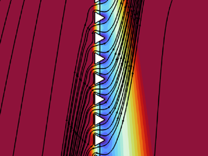
4.2. Configuration $C2$: capturing solute concentration jumps across membranes

In figure 5(b), a permeable Janus membrane is invested by a uniform Stokes flow orthogonal to the membrane itself, which transports a solute of concentration  $c$ at ${Pe}=100$. The membrane is formed by the repetition of the microscopic structure $GF1$. At the inlet, a constant concentration $c=1$ is imposed, while the upper and lower boundaries of the fluid domain absorb the solute at a given flow rate $\kappa =\epsilon$. The macroscopic flow is symmetric with respect to the axis $x_3=0$ (figure 5b). The vertical velocity and concentration fields (figures 7a,b) show noticeable variations through the pores. These microscopic fast variations along the normal to the membrane direction find their macroscopic counterpart in the jumps experienced by the tangential velocity $u_3$, the solute concentration c and the pressure p (figures 7d,e,g). The upward half of each solid inclusion produces larger viscous dissipation, implying a slip velocity smaller than its downward counterpart since $|\mathcal {M}_{ttn}^{-}|<|\mathcal {N}_{ttn}^+|$ in this case. The values of concentration at the membrane in figures 7(e,f) are deviations from $C_0$ (see (2.15)), which in the present case is identically zero. Contrary to the continuous interface condition (2.12) (maroon), the Janus model quantifies perfectly the jump in the concentration field (yellow and purple). In particular, the continuous interface condition underestimates (resp. overestimates) the concentration value in the upward (resp. downward) far-field region, producing non-negligible local errors between the macroscopic model and the fully resolved solution. The upward exposed surface of the solid inclusion is larger than its downward counterpart, thus producing larger macroscopic, averaged deviations of the upward concentration from $C_0$. The benefit given by the Janus model in the evaluation of the concentration jump is instead negligible at the scale of the pressure jump (order $\epsilon ^0$) since only modifications of order $\epsilon$ are produced by the asymmetry of the microstructure. We also notice that the maroon profile in figure 7(h) is calculated a posteriori using (2.11), and it is not needed to find the pressure field in the macroscopic domain, which is set by the velocity interface conditions (2.10). We finally conclude our analysis by observing that the streamwise velocity $u_1$ sampled on $\mathbb {C}^\pm$ (figure 7c) is continuous since, as observed already in § 3, $|\mathcal {M}_{nnn}^{\pm }|=|\mathcal {N}_{nnn}^{\pm }|$.

Figure 7. Flow configuration  $C2$. (a,b) Isocontours of full-scale solvent pressure and solute concentration field across two solid inclusions, together with the solvent flow streamlines (black lines). (c–e,g) Horizontal velocity, vertical velocity, concentration and pressure fields sampled on $\mathbb {C}$. (f,h) Concentration and pressure fields sampled over the line $x_3=0$ orthogonal to $\mathbb {C}$.
5. Conclusions and perspectives
The introduction of upward and downward averages within the homogenization framework to describe the flow across a microstructured Janus membrane revealed a discontinuous nature of the macroscopic flow field. In particular, the solute–solvent flow behaviour is led back to the solution of simple microscopic problems resulting from different forcings and averages on the two sides of the membrane. The model developed extends the initial model introduced in Zampogna & Gallaire (Reference Zampogna and Gallaire2020) and Zampogna et al. (Reference Zampogna, Ledda and Gallaire2022) to a larger class of thin porous membranes, whose properties may exhibit fast variations along the filtration direction within a single pore. We developed a rigorous framework identifying the essential features of Janus membranes, which represent a key finding in current membrane technology. In a design perspective, a possible development is the maximization of the differences between the upward and downward averages of the microscopic quantities. These quantities can be employed as control parameters of the flow; see e.g. Ledda et al. (Reference Ledda, Boujo, Camarri, Gallaire and Zampogna2021) for the case of symmetric membranes. This model is a first but crucial step in the macroscopic description of phenomena based on (electro-)phoresis (Michelin & Lauga Reference Michelin and Lauga2014; Aubret, Ramananarivo & Palacci Reference Aubret, Ramananarivo and Palacci2017). In this chemico-physical framework, the jump in the concentration field constitutes the main drive for the fluid flow, therefore calling for the extension of the model to the case of bidirectional solvent–solute coupling, where the solute flow induces a solute flux, and vice versa. In conclusion, the employment of downward and upward averages for Janus membranes within the homogenization framework gives a rigorous foundation to quantify the effective properties of real, partially permeable membranes that at present are determined mainly from heuristic considerations (Kedem & Katchalsky Reference Kedem and Katchalsky1958), opening for a predictive analysis of the transport through real membranes.
Funding
This work was supported by the Swiss National Science Foundation (G.A.Z., grant no. PZ00P2_193180).
Declaration of interests
The authors report no conflict of interest.
Appendix A. Determination of the base value of the concentration $C_0$ at the membrane

The use of the interface conditions (2.12) and (2.15) relies on the knowledge of the quantity  $C_0$. Zampogna et al. (Reference Zampogna, Ledda and Gallaire2022) have shown that this quantity is equal to $C^{\partial \mathbb {M}}$ if $\lambda \neq 0$ in (2.2a,b). Conversely, when $\lambda =0$, $C_0$ can be found by solving a macroscopic flow configuration where the advective velocity at the membrane is calculated via (2.10), while the conditions imposed on $\mathbb {C}$ are
 \begin{equation} \zeta_i(F_{i}\vert_{\mathbb{C^-}}-F_{i}\vert_{\mathbb{C^+}})= {\kappa}_{eff}\,\eta {c}\vert_{\mathbb{C}},\quad c\vert_{\mathbb{C}^-}=c\vert_{\mathbb{C}^+}, \end{equation}
where  ${\kappa }_{eff}=\kappa \,|\partial \mathbb {M}|$, and $|\partial \mathbb {M}|$ is the total surface of the microstructured membrane. We refer to Zampogna et al. (Reference Zampogna, Ledda and Gallaire2022) for further mathematical details about the development of condition (A1).


 Open access