


1. Introduction
Shock waves play an important role in supersonic mixing and combustion. For instance, Marble (Reference Marble1994) and Yu et al. (Reference Yu, He, Zhang and Liu2020) inherently investigated the interaction between an oblique shock wave and a fuel jet. The effect of a shock/spanwise-vortex interaction on mixing enhancement was demonstrated using a strut hydrogen-fuel injector (Huang et al. Reference Huang, Du, Yan and Moradi2018; Soni & De Reference Soni and De2018). The use of streamwise vortices generated by physical devices (e.g. ramps, pylons, struts and lobed mixers) is a promising approach for enhancing the mixing of fuel and air in a supersonic flow because the vortices can mitigate compressibility effects (Sandham & Reynolds Reference Sandham and Reynolds1991; Morkovin Reference Morkovin1992; Lele Reference Lele1994; Naughton, Cattafesta & Settles Reference Naughton, Cattafesta and Settles1997; Hiejima Reference Hiejima2013, Reference Hiejima2019). Among these devices, the hypermixer struts mounted in the centre of a channel or combustor, which can generate supersonic streamwise vortices, have excellent mixing and combustion capabilities in supersonic flows (Settles Reference Settles1991; Waitz et al. Reference Waitz1997; Gerlinger et al. Reference Gerlinger, Stoll, Kindler, Schneider and Aigner2008; Burns et al. Reference Burns, Koo, Kim, Clemens and Raman2011; Fureby et al. Reference Fureby, Nordin-Bates, Petterson, Bresson and Sabelnikov2015; Hiejima & Oda Reference Hiejima and Oda2020). Further, the advantages of strut-type injections with streamwise vortices on supersonic mixing and transition were summarised (Hwang & Min Reference Hwang and Min2022).
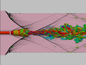
Interactions between streamwise vortex and shock wave inducing vortex breakdown, also called shock-induced vortex breakdown, are another important point. Zatoloka, Ivanyushkin & Nikolayev (Reference Zatoloka, Ivanyushkin and Nikolayev1978) first investigated the effect of these interactions on the inlet performance of a supersonic vehicle. Figure 1 shows the vortex breakdown caused by the interaction between a streamwise vortex and crossing of shocks using the hypermixer strut. Then, as the vortex breakdown induced by adverse pressure gradients based on shock waves created subsonic regions, a bubble-type breakdown appeared around their cross-point (Hiejima Reference Hiejima2016a). This phenomenon is essentially similar to a subsonic vortex breakdown. The physical features of vortex breakdown include a sudden increase in the vortex core size, reversed flow and stagnation points, and highly unstable structures (Hall Reference Hall1972; Delery et al. Reference Delery, Horowitz, Leuchter and Solignac1984; Leibovich Reference Leibovich1984; Escudier Reference Escudier1988; Lucca-Negro & O'Doherty Reference Lucca-Negro and O'Doherty2001). The onset of the breakdown is subject to various influences of swirl intensity, adverse pressure gradients and formation of a stagnation point near the axis. In particular, the swirl number highly affects the breakdown condition in incompressible flows. Hall (Reference Hall1972) defined a vortex breakdown as an abrupt change in the vortex structure with very pronounced retardation of the flow along the axis and a corresponding divergence of the stream surfaces near the axis. According to Leibovich (Reference Leibovich1978), a stagnation point is required for vortex breakdown. As first described by Lambourne & Bryer (Reference Lambourne and Bryer1961), the breakdown configuration is categorised into bubble-type (axisymmetric shape) and spiral-type (non-axisymmetric shape). Note that transitions exist between bubble- and spiral-type vortex breakdowns and are affected by changes in swirl intensity and Reynolds number.

Figure 1. Contours of the density gradient for the flow around a hypermixer strut at Mach number 3.5; side view. This is a separation-restraint strut (Hiejima & Nishimura Reference Hiejima and Nishimura2021) that can induce downstream streamwise vorticity to enhance supersonic mixing and combustion in the application of the interaction with shocks.
Shock-induced vortex breakdown was detailed by Delery (Reference Delery1994) and Kalkhoran & Smart (Reference Kalkhoran and Smart2000). The interactions were mainly examined for normal shock wave and vortex interactions (NSVIs) and oblique shock wave and vortex interactions (OSVIs). Early experiments on vortex breakdown based on the NSVI detected three types of interactions, namely weak, moderate and strong, by comparing the size of the interaction region with that of the diameter of the upstream vortex core (Metwally, Settles & Horstman Reference Metwally, Settles and Horstman1989; Cattafesta & Settles Reference Cattafesta and Settles1992; Delery Reference Delery1994). Several numerical studies of the NSVI have also been conducted by Metwally et al. (Reference Metwally, Settles and Horstman1989), Meadows, Kumar & Hussaini (Reference Meadows, Kumar and Hussaini1991), Kandil, Kandil & Liu (Reference Kandil, Kandil and Liu1993), Erlebacher, Hussaini & Shu (Reference Erlebacher, Hussaini and Shu1997) and Zhang, Zhang & Shu (Reference Zhang, Zhang and Shu2009). In these studies, numerical visualisations revealed the flow field within the interaction region, which is difficult to achieve experimentally.
In OSVI experiments, Smart, Kalkhoran & Popovic (Reference Smart, Kalkhoran and Popovic1998) and Kalkhoran & Smart (Reference Kalkhoran and Smart2000) demonstrated that the vortex breakdown region experiences subsonic speeds. Klaas, Schröder & Althaus (Reference Klaas, Schröder and Althaus2005) measured the axial and tangential Mach number profiles in OSVI through laser Doppler velocimetry and particle image velocimetry. Thompson et al. (Reference Thompson, Kiriakos, Pournadali Khamseh and DeMauro2022) investigated weak and moderate OSVIs through stereoscopic particle image velocimetry. They determined that only moderate interactions produce conical shock distortions. Recently, Wei et al. (Reference Wei, Liu, Wang, Zhao and Yang2022a) splendidly captured helical structures downstream in strong OSVI. They found that turbulent mixing drastically increases behind the interaction through nanoparticle-based planar laser scattering technology. OSVI has also been numerically investigated by Corpening & Anderson (Reference Corpening and Anderson1989), Nedungadi & Lewis (Reference Nedungadi and Lewis1996), Rizzetta (Reference Rizzetta1997), Thomer, Schröder & Krause (Reference Thomer, Schröder and Krause2001), Zheltovodov, Pimonov & Knight (Reference Zheltovodov, Pimonov and Knight2007), Magri & Kalkhoran (Reference Magri and Kalkhoran2013), Hiejima (Reference Hiejima2014) and Wei et al. (Reference Wei, Yang, Liu, Zhao, Wang and Sun2022b). Several studies have shown that characteristic vortical structures (e.g. helices) are generated because of the shock–vortex interaction. According to a previous study (Hiejima Reference Hiejima2014), these structures strongly indicate that the breakdown configuration relies on upstream conditions (the free stream Mach number, vortex circulation, axial velocity deficit and shock angle). The circulation (swirl intensity) in an upstream vortex is crucial to vortex breakdown even in supersonic flows.
Regarding an upstream vortex, the vortex breakdown phenomenon is closely related to flow instability (Ludwieg Reference Ludwieg1960; Leibovich Reference Leibovich1984). Flow fields in vortex breakdown are subjected to modes with low azimuthal wavenumbers (Ruith et al. Reference Ruith, Chen, Meiburg and Maxworthy2003; Oberleithner et al. Reference Oberleithner, Sieber, Nayeri, Paschereit, Petz, Hege, Noack and Wygnanski2011; Hiejima Reference Hiejima2017). Herrada, Pérez-Saborid & Barrero (Reference Herrada, Pérez-Saborid and Barrero2003) demonstrated that the critical swirl number for the onset of vortex breakdown increased with the Mach number. Rusak & Lee (Reference Rusak and Lee2002) indicated that with the increase in the Mach number, a bubble breakdown of compressible vortices was delayed. Conversely, Luginsland (Reference Luginsland2015) determined that with the increase in the Mach number, the critical swirl number in subsonic flows decreased. Assuming that a vortex breakdown occurs because of a process similar to hydraulic jumps and shock waves, an inviscid vortex breakdown is regarded as a transition between two conjugate flow states (Benjamin Reference Benjamin1962; Mager Reference Mager1972). Based on this concept, Hiejima (Reference Hiejima2018) indicated the conditions for the occurrence of vortex breakdown in supersonic flows without shocks and found that the breakdown occurs without a stagnation point and subsonic region. Further, vortex breakdown is due to instability in helicity under strong swirl conditions (Hiejima Reference Hiejima2020). Therefore, as a difference exists between incompressible and compressible vortex breakdowns without shock interactions, bubble structures in shock-induced vortex breakdowns may differ from those in incompressible breakdowns.
This study aims to clarify how bubble vortex breakdown is caused by the interaction between a streamwise vortex and the crossing of shock waves as a stronger factor than an oblique shock. As the breakdown mechanism related to the intersection of oblique shocks remains unknown, a key feature for the onset of the breakdown should be extracted. In this study, spatial evolutions of streamwise vortices with shock interaction were investigated numerically for varying Mach numbers, shock angles and vortex circulation values.
The remainder of this paper is organised as follows. The intersection of the crossing of shock waves is accounted for in terms of the shock polar and a supersonic streamwise vortex is described as an upstream vortex in § 2. The method and computational conditions of direct numerical simulations are described in § 3. The results of the interaction between the vortex and crossing of shock waves related to vortex breakdown are provided and discussed in § 4. In addition, through numerical simulations, this section clarifies the effects of the interaction phenomenon on the vortex breakdown for various values of shock angle and vortex circulation. Furthermore, the section presents the threshold for a bubble vortex breakdown, derived and verified based on numerical results. Finally, conclusions are presented in § 5.
2. Basic elements of a flow field study
2.1. Intersection of oblique shocks
This subsection discusses the intersection of oblique shock waves without a streamwise vortex at Mach number  $M_1$. Figure 2(a) presents the schematic of the situation. Incident shocks due to deflection angle $\theta$ continue as reflected shocks downstream of the intersection. Note that the shock angle is defined as $\beta$ and subscripts 1, 2 and 3 are subjected to each state in figure 2(a). Depending on $M_1$ and $\theta$, the appearance of two shock-wave reflection configurations is mainly called regular reflection (RR) and Mach reflection (MR) in figures 2(a) and 2(b), respectively.

Figure 2. Schematic of (a) regular reflection (RR) and (b) Mach reflection (MR). (c) Domains of possible reflection configuration in the ( $M_1$– $\beta$) plane. Note that the blue line denotes $\beta _1^{A} = \sin ^{-1}(1/M_1)$, the red line $\beta _1^{N}$ is the mechanical-equilibrium criterion, the red dashed line $\beta _1^{D}$ is the detachment criterion and the black line $\beta _1^{B}$ is $M_2 = 1$. On theoretical grounds, only RR is possible within $\beta _1^{A} < \beta < \beta _1^{N}$, only MR is possible within $\beta _1^{D} < \beta < \beta _1^{B}$, and both RR and MR are possible within the intermediate range $\beta _1^{N} < \beta < \beta _1^{D}$. Shock polar (pressure-deflection diagram) illustrating the flow regions at (d) $M_1 = M_\infty (1 - \mu ) = 2.38$ and (e) $M_1 = M_\infty (1 - \mu ) = 3.4$, with various (2)-polars.
A shock polar (also called the pressure-deflection diagram) should be introduced to understand some of these interactions; it is the same as the locus of all possible static pressures  $p$ behind an oblique shock wave as a function of deflection angle $\theta$ for given upstream conditions (Anderson Reference Anderson2003). The shock polar comprises the (1)-polar and (2)-polar in this system. In the (1)-polar case, as $M_1$ and $p_1$ are known, the relation between $p$ and $\theta$ is given by
 \begin{equation} \tan\theta =\frac{\displaystyle\frac{p}{p_1}-1}{1+\gamma M_1^2-\displaystyle\frac{p}{p_1}}\sqrt{\frac{\displaystyle\frac{2\gamma M_1^2-(\gamma-1)}{\gamma+1}-\displaystyle\frac{p}{p_1}}{\displaystyle\frac{p}{p_1}+\displaystyle\frac{\gamma-1}{\gamma+1}}}, \end{equation}
where  $\gamma$ is the ratio of specific heats. Then, the (1)-polar is obtained as $\theta =f({p}/{p_1})$ from (2.1). Subsequently, when determining value $\theta = \theta '$, $\beta$ and $M_2$ are determined using (2.2) and (2.3), respectively,
 $$\begin{gather} \tan\theta' =\frac{2\cot\beta(M_1^2\sin^2\beta-1)}{M_1^2(\gamma+\cos 2\beta)+2}, \end{gather}$$
 $$\begin{gather}M_2^2=\frac{1}{\sin^2(\beta-\theta')}\frac{(\gamma-1)M_1^2\sin^2\beta+2}{2\gamma\,M_1^2\sin^2\beta-(\gamma-1)}. \end{gather}$$
Based on  $\beta$, $p_2$ is uniquely identified by
 \begin{equation} \frac{p_2}{p_1}=1+\frac{2\gamma}{\gamma+1}(M_1^2\sin^2\beta-1). \end{equation}
In the (2)-polar starting at  $p_2$ and $\theta '$, the relation between $p$ and $\theta _r$ (figure 2a) is given by
 \begin{equation} \tan(-\theta_r) =\frac{\displaystyle\frac{p}{p_2}-1}{1+\gamma M_2^2-\displaystyle\frac{p}{p_2}}\sqrt{\frac{\displaystyle\frac{2\gamma M_2^2-(\gamma-1)}{\gamma+1}-\displaystyle\frac{p}{p_2}}{\displaystyle\frac{p}{p_2}+\displaystyle\frac{\gamma-1}{\gamma+1}}}. \end{equation}
The (2)-polar begins at  $\theta '$ and is plotted using ${p}/{p_1} = ({p}/{p_2})({p_2}/{p_1})$ obtained from (2.4) and (2.5). Then, given $M_2$, $\theta _r =f({p}/{p_1})$. Thus, the shock polar is used to graphically determine the possibility of RR or the possibility of MR.
Figure 2(c) shows the domains of possible reflection configurations in the ( $M_1$– $\beta$) plane (Hornung Reference Hornung1986; Ben-Dor Reference Ben-Dor2007). The detachment and mechanical-equilibrium criteria are well known for reflection. The detachment criterion is obtained when the (2)-polar is tangent to the $p$-axis. The mechanical-equilibrium criterion is defined as follows: the (2)-polar intersects the $p$-axis exactly at the normal shock point of the (1)-polar. For example, as seen in figure 2(d), the (1)-polar is denoted by the red curve, whereas the remaining curves denote the (2)-polar. Note that only RR is possible within the $\beta _1^{A} < \beta < \beta _1^{N}$ range and only MR is possible within the $\beta _1^{D} < \beta < \beta _1^{B}$ range. In the intermediate range $\beta _1^{N} < \beta < \beta _1^{D}$, both RR and MR are possible, known as the dual-solution domain. The transition between the RR and MR of shock waves is also well known (Ivanov et al. Reference Ivanov, Vandromme, Fomin, Kudryavtsev, Hadjadj and Khotyanovsky2001). Figures 2(d) and 2(e) show the shock polars based on the Mach number conditions (table 1) addressed in this study using (2.1) to (2.5). Note that at the centreline, the upstream Mach number is not $M_\infty$ but $M_\infty (1 - \mu )$, considering the vortex centre (see (2.8c)). The mechanical-equilibrium criterion is that $\beta _c = 40.50^\circ$ ( $\theta _c = 16.73^\circ$) for $M_1 = 2.38$ and $\beta _c = 35.61^\circ$ ( $\theta _c = 20.42^\circ$) for $M_1 = 3.4$. Their cases are also plotted together in figures 2(d) and 2(e), respectively. As mentioned previously, the criterion indicates that the (1)-polar intersects the (2)-polar on the $p$-axis. If the lower intersection of the (2)-polar is less than the upper intersection of the (1)-polar on the $p$-axis, RR occurs. If the lower intersection of the (2)-polar is more than the upper intersection of the (1)-polar on the $p$-axis, MR occurs. Note that here is out of consideration of expansion waves that always occur in the computational domain, as presented in figure 3.
Table 1. Computational conditions.


Figure 3. Configuration of the computational domain from the lateral ( $x$–
$x$– $y$ plane) and rear ( $y$–
$y$– $z$ plane) views. The flow field includes a streamwise vortex and a double oblique-shock wave.
2.2. Supersonic streamwise vortices
The density, three velocity components, pressure, temperature and entropy are expressed in  $x_i^*$ coordinates as $\rho ^*$, $u_i^*$, $p^*$, $T^*$ and $s^*$, respectively (note that dimensional quantities are superscripted with asterisks). The reference length of a streamwise vortex is defined as $\delta _s^*$, which denotes swirl thickness obtained from $\varGamma ^* = ({\rm \pi} \delta ^*_s)\omega _{x, {max}}^*$. Here, $\omega _{x, {max}}^*$ and $\varGamma ^*$ denote the maximum axial vorticity and total circulation of the entire distributed axial vorticity, respectively. By using the free stream sonic velocity $c_{\infty }^*(= \sqrt {\gamma R^*\,T_\infty ^*})$ and density $\rho _{\infty }^*$, the physical variables can be normalised as follows:
 \begin{align}
\rho&=\frac{\rho^*}{\rho_{\infty}^*},\quad
u_i=\frac{u_i^*}{c_{\infty}^*},\quad
p=\frac{p^*}{\rho_{\infty}^*c_{\infty}^{*2}},\quad
T=\frac{T^*}{\gamma T_{\infty}^*}, \nonumber\\
s&=\frac{s^*}{C_v^*},\quad
x_i=\frac{x_i^*}{\delta_s^*},\quad
t=\frac{c_{\infty}^*}{\delta_s^*}\,t^*,
\end{align}
\begin{align}
\rho&=\frac{\rho^*}{\rho_{\infty}^*},\quad
u_i=\frac{u_i^*}{c_{\infty}^*},\quad
p=\frac{p^*}{\rho_{\infty}^*c_{\infty}^{*2}},\quad
T=\frac{T^*}{\gamma T_{\infty}^*}, \nonumber\\
s&=\frac{s^*}{C_v^*},\quad
x_i=\frac{x_i^*}{\delta_s^*},\quad
t=\frac{c_{\infty}^*}{\delta_s^*}\,t^*,
\end{align}
where  $t^*$ denotes the time, $R^*$ is the gas constant, $T_\infty ^*$ is the free stream temperature and $C_v^* = R^*/(\gamma -1)$ represents the specific heat at a constant volume. Here, the free stream Mach number $M_\infty$ and Reynolds number $Re$ are defined as
 \begin{equation} M_\infty = \frac{u_{\infty}^*}{c_{\infty}^*},\quad {Re} = \frac{\rho_{\infty}^*u_{\infty}^*\delta_s^*}{\eta_{\infty}^*}, \end{equation}
where  $u_\infty ^*$ is the free stream velocity and $\eta _{\infty }^*$ is the viscosity.
To examine the interaction between crossing oblique shock waves and a streamwise vortex, Batchelor vortices (Batchelor Reference Batchelor1964) are used as an upstream vortex, because their profiles are compatible with many experimental swirling flows at high Reynolds numbers (Cattafesta & Settles Reference Cattafesta and Settles1992; Naughton et al. Reference Naughton, Cattafesta and Settles1997; Wang & Sforza Reference Wang and Sforza1997; Kalkhoran & Smart Reference Kalkhoran and Smart2000). Upstream streamwise vortices are assumed to be steady and axisymmetric. In cylindrical polar coordinates ( $r, \theta, x$), the radial, azimuthal and axial velocities (denoted by $u_r$, $u_\theta$ and $u_x$, respectively) of the Batchelor vortex are denoted as follows:
 \begin{align} u_r(r) &= 0,\quad u_\theta(r) = M_\infty\displaystyle\frac{q}{r}[1-\exp({-r^2})],\quad u_x(r) = M_\infty[1 - \mu \exp({-r^2})], \end{align}
where  $q$ and $\mu$ denote the circulation (swirl intensity) and axial velocity deficit, respectively. In incompressible flows, a streamwise vortex with a large circulation required for vortex breakdown is easy to generate. Conversely, in compressible flows, a streamwise vortex with a large circulation (i.e. strong swirl) is difficult to generate owing to the incidence of shock waves or separation on a device. According to the devices that generate a Batchelor-type vortex in supersonic flows (Naughton et al. Reference Naughton, Cattafesta and Settles1997; Hiejima Reference Hiejima2016b; Wu et al. Reference Wu, He, Yu and Liu2022), the maximum swirl intensity is approximately $q \approx 0.34$, which also depends on the free stream Mach number. The axial velocity deficit is roughly $0.5$– $0.8$ behind the device that generated the vortex and is similar to a wake flow. However, axial velocity profiles recover the deficit in wake flows downstream, far from the device. In this study, the deficit $\mu = 0.32$ based on previous measurements (Hiejima Reference Hiejima2013).
Thermodynamic profiles in a compressible Batchelor vortex are poorly understood because their measurements are rare. At high Reynolds numbers, free stream flows do not appreciably depend on viscosity; hence, they can reasonably be regarded as inviscid supersonic flows. The entropy equation is defined as
 \begin{equation} s = \log_e\left(\frac{p}{\rho^\gamma}\right) + \mbox{const.} \end{equation}
Furthermore, Crocco's theorem is expressed as follows (Crocco Reference Crocco1937):
 \begin{equation} \frac{1}{\gamma-1}T\,\frac{{\rm d}s}{{\rm d} r}= \frac{\gamma}{\gamma-1}\frac{{\rm d} T_0}{{\rm d} r} - u_\theta\omega_x + u_x\omega_\theta, \end{equation}
where  $T_0$ is the total temperature, and $\omega _x$ and $\omega _\theta$ are the axial and azimuthal vorticities, respectively. Experiments have shown that $T_0$ is approximately uniform (Cattafesta & Settles Reference Cattafesta and Settles1992). Nedungadi & Lewis (Reference Nedungadi and Lewis1996) and Wei et al. (Reference Wei, Yang, Liu, Zhao, Wang and Sun2022b) also applied this assumption in numerical simulations. In this study, ${\rm d}s/{\rm d}r$ was derived by setting ${{\rm d}T_0/{\rm d}r = 0}$ in (2.10). By using a radial momentum equation and the entropy derivation, the density and pressure required for compressible flows in basic inviscid steady flow are related as follows:
 \begin{equation} \frac{{\rm d} p}{{\rm d} r} = {\rho}\frac{{u_{\theta}}^2}{r} ,\quad \frac{{\rm d} \rho}{{\rm d} r} = \frac{\rho}{\gamma}\left(\frac{1}{p}\frac{{\rm d} p}{{\rm d} r} -\frac{{\rm d} s}{{\rm d} r}\right). \end{equation}
Density  $\rho (r)$ and pressure $p(r)$ profiles are obtained by solving the ordinary differential equations (2.10) and (2.11a,b).
Erlebacher et al. (Reference Erlebacher, Hussaini and Shu1997), Thomer et al. (Reference Thomer, Schröder and Krause2001) and Zhang et al. (Reference Zhang, Zhang and Shu2009) used a Taylor vortex (Ragab & Sreedhar Reference Ragab and Sreedhar1995) with the addition of an isentropic condition as the upstream vortex. As this profile has a negative vorticity and involves centrifugal instability, a larger circulation will result in a more instability. Thus, Batchelor and Taylor vortices differ in their nature of instability. Note that the velocity profiles of the upstream vortex affect the onset of vortex breakdown.
3. Numerical formulations
3.1. Governing equations
From the perspective of vortex breakdown, the spatial evolution of streamwise vortices activated by the interaction with the intersection of oblique shocks is investigated through numerical simulations. The normalised governing equations are three-dimensional, unsteady, compressible Navier–Stokes equations in general coordinates  $\xi _i$ ( $i = 1\unicode{x2013}3$). These are denoted as
 \begin{gather} \frac{\partial{}}{\partial{t}}\left(\frac{\boldsymbol{Q}}{J}\right) + \frac{\partial{\boldsymbol{F}_i}}{\partial{\xi_i}}= \frac{\partial{\boldsymbol{F}_{vi}}}{\partial{\xi_{i}}}, \end{gather}
 \begin{gather}
\left.\begin{gathered} {\boldsymbol{Q}} =
\left[\begin{array}{@{}c@{}} \rho \\ \rho u_1 \\ \rho u_2 \\ \rho
u_3 \\ e \end{array} \right],\quad {\boldsymbol{F}}_i =
\left[ \begin{array}{@{}c@{}} \rho U_i\\ \rho u_1 U_i +
p(J^{{-}1}\partial\xi_i/\partial x_1)\\ \rho u_2 U_i +
p(J^{{-}1}\partial\xi_i/\partial x_2)\\ \rho u_3 U_i +
p(J^{{-}1}\partial\xi_i/\partial x_3)\\ (e + p)U_i
\end{array} \right],\quad {\boldsymbol{F}}_{vi} = \left[
\begin{array}{@{}c@{}} 0 \\
\textsf{$\mathit{\tau}$}_{1k}(J^{{-}1}\partial\xi_i/\partial x_k) \\
\textsf{$\mathit{\tau}$}_{2k}(J^{{-}1}\partial\xi_i/\partial x_k) \\
\textsf{$\mathit{\tau}$}_{3k}(J^{{-}1}\partial\xi_i/\partial x_k) \\
\beta_k(J^{{-}1}\partial\xi_i/\partial x_k) \\ \end{array}
\right], \\ J^{{-}1}=\frac{\partial
x_1}{\partial\xi_1}\left(\frac{\partial
x_2}{\partial\xi_2}\frac{\partial
x_3}{\partial\xi_3}-\frac{\partial
x_2}{\partial\xi_3}\frac{\partial
x_3}{\partial\xi_2}\right) + \frac{\partial
x_1}{\partial\xi_2}\left(\frac{\partial
x_2}{\partial\xi_3}\frac{\partial x_3}{\partial\xi_1}-
\frac{\partial x_2}{\partial\xi_1}\frac{\partial
x_3}{\partial\xi_3}\right) \\ \quad+ \frac{\partial
x_1}{\partial\xi_3} \left(\frac{\partial
x_2}{\partial\xi_1}\frac{\partial
x_3}{\partial\xi_2}-\frac{\partial x_2}{
\partial\xi_2}\frac{\partial x_3}{\partial\xi_1}\right),\\
U_i = \left({J^{{-}1}}\frac{\partial \xi_i}{\partial
x_k}\right)u_k,\quad \beta_i = u_k\textsf{$\mathit{\tau}$}_{ik}+q_i,
\end{gathered}\right\} \end{gather}
\begin{gather}
\left.\begin{gathered} {\boldsymbol{Q}} =
\left[\begin{array}{@{}c@{}} \rho \\ \rho u_1 \\ \rho u_2 \\ \rho
u_3 \\ e \end{array} \right],\quad {\boldsymbol{F}}_i =
\left[ \begin{array}{@{}c@{}} \rho U_i\\ \rho u_1 U_i +
p(J^{{-}1}\partial\xi_i/\partial x_1)\\ \rho u_2 U_i +
p(J^{{-}1}\partial\xi_i/\partial x_2)\\ \rho u_3 U_i +
p(J^{{-}1}\partial\xi_i/\partial x_3)\\ (e + p)U_i
\end{array} \right],\quad {\boldsymbol{F}}_{vi} = \left[
\begin{array}{@{}c@{}} 0 \\
\textsf{$\mathit{\tau}$}_{1k}(J^{{-}1}\partial\xi_i/\partial x_k) \\
\textsf{$\mathit{\tau}$}_{2k}(J^{{-}1}\partial\xi_i/\partial x_k) \\
\textsf{$\mathit{\tau}$}_{3k}(J^{{-}1}\partial\xi_i/\partial x_k) \\
\beta_k(J^{{-}1}\partial\xi_i/\partial x_k) \\ \end{array}
\right], \\ J^{{-}1}=\frac{\partial
x_1}{\partial\xi_1}\left(\frac{\partial
x_2}{\partial\xi_2}\frac{\partial
x_3}{\partial\xi_3}-\frac{\partial
x_2}{\partial\xi_3}\frac{\partial
x_3}{\partial\xi_2}\right) + \frac{\partial
x_1}{\partial\xi_2}\left(\frac{\partial
x_2}{\partial\xi_3}\frac{\partial x_3}{\partial\xi_1}-
\frac{\partial x_2}{\partial\xi_1}\frac{\partial
x_3}{\partial\xi_3}\right) \\ \quad+ \frac{\partial
x_1}{\partial\xi_3} \left(\frac{\partial
x_2}{\partial\xi_1}\frac{\partial
x_3}{\partial\xi_2}-\frac{\partial x_2}{
\partial\xi_2}\frac{\partial x_3}{\partial\xi_1}\right),\\
U_i = \left({J^{{-}1}}\frac{\partial \xi_i}{\partial
x_k}\right)u_k,\quad \beta_i = u_k\textsf{$\mathit{\tau}$}_{ik}+q_i,
\end{gathered}\right\} \end{gather}
where  ${\boldsymbol {Q}}$ is a vector of conservative variables, and ${\boldsymbol {F}}_i$ and ${\boldsymbol {F}}_{vi}$ contain the convective and viscous fluxes, respectively. The Jacobian $J$ transforms the coordinate system from a physical space to a computational space, where $J^{-1}\partial \xi _i/\partial x_k$ represents the derivatives of the coordinate conversion (i.e. the metrics) and $U_i$ is the velocity component at the grid interface. The thermodynamics relation, normalised equation of state and transport coefficients are given as follows:
 \begin{equation} \left.\begin{gathered} e = \frac{p}{\gamma-1} + \frac{1}{2}\rho u_ku_k, \\ p = \rho T, \\ \textsf{$\mathit{\tau}$}_{ij}=\frac{\eta(T)}{{{Re}_M}}\left(\frac{\partial{u_i}}{\partial{x_j}}+\frac{\partial{u_j}}{\partial{x_i}}-\frac{2}{3} \delta_{ij}\frac{\partial{u_k}}{\partial{x_k}}\right),\quad q_i ={-}\frac{\gamma}{(\gamma-1)}\frac{\eta(T)}{{{Re}_M\,{Pr}}} \frac{\partial{T}}{\partial{x_i}}, \end{gathered}\right\} \end{equation}
where  $e$ is the total energy, $\textsf{$\mathit{\tau}$} _{ij}$ is the viscous stress tensor, $q_i$ is the conductive heat flux and $u_i$ represents the velocity components in the Cartesian coordinates. The Reynolds number based on sonic velocity is defined as ${Re}_M = (\rho _\infty ^* c_\infty ^* \delta _s^*)/\eta _\infty ^*$ ( $= Re/M_\infty$) and the Prandtl number $Pr$ is 0.72. Viscosity $\eta (T)$ is calculated from Sutherland's law as a function of the static temperature (Schlichting Reference Schlichting1979):
 \begin{equation} \eta(T)=\sqrt{\gamma} T^{{3}/{2}}\frac{1 + \gamma{\vartheta}}{T + {\vartheta}}, \end{equation}
where  ${\vartheta } = 110.4/(\gamma T_\infty ^*)$ is normalised by a free stream temperature.
3.2. Numerical methods and computational conditions
This study aims to investigate vortex breakdown due to the interaction with the intersection of shocks. To capture this phenomenon, simulations of vortical structures that evolve in supersonic flows with shock waves must be highly accurate. A convective flux was evaluated by the type of advection upstream splitting method (AUSM, a flux-splitting technique) called the AUSMDV scheme (Wada & Liou Reference Wada and Liou1994) and the weighted compact nonlinear scheme (WCNS). Note that strong discontinuities, such as shock waves, were observed in this system. As a shock-capturing simulation with high accuracy, primitive variables at the grid interfaces were interpolated to the ninth-order accuracy using WCNS-JS (Hiejima Reference Hiejima2022) that combined certain substencils of the original targeted essentially non-oscillatory scheme (Fu, Hu & Adams Reference Fu, Hu and Adams2016) and weight coefficients (Jiang & Shu Reference Jiang and Shu1996). Viscous flux terms were calculated to the eighth-order accuracy by using a central difference method. The temporal integration adopted a four-step, fourth-order accuracy scheme (Jameson, Schmidt & Turkel Reference Jameson, Schmidt and Turkel1981).
The computational domain comprises a rectangular duct including a constrictive ramp with ramp angle  $\theta$ to generate oblique shock, as shown in figure 3. In the same configuration, Su et al. (Reference Su, Wen, Li, Wan, Han, Wang and Wang2022) used the symmetrical wedge as a shock-wave generator to investigate the RR and MR. The streamwise vortex defined in § 2.2 was introduced from the centre in the $y$–
$y$– $z$ plane at $x = 0$. Note that distance $X_\theta = 17/\tan \beta$, i.e. $X_\theta$ varies depending on shock angle $\beta$. In addition, the grid spacing $\Delta x$ was uniform in the $x$ direction. In the $y$ and $z$ directions, the grid was clustered to resolve the interaction between a streamwise vortex and shock waves. Grid spacing $\Delta y\ (=\Delta z)$ was uniform inside the five inner vortex-core diameters near the vortex axis. In the adjoining region, it gradually increased over a space that extended 5–10 times the radius of the vortex core. Outside the region, the grid spacing reached a maximum of three times the inner grid spacing. Note that the vortex core radius was close to the radial distance of the maximum azimuthal velocity.
Supersonic inflows were introduced in the  $x$ direction and fixed Batchelor vortices at $M_\infty = 3.5$ and $5.0$, and ${Re}_M = 9000$. The outflow condition at $x = 110 + X_\theta$ was extrapolated to the zeroth order. Furthermore, slip wall conditions were imposed on boundary surfaces comprising the $x$–
$x$– $y$ and $x$–
$x$– $z$ planes because in this study, the effect of the boundary layer near the wall was almost insignificant. Table 1 lists the computational parameters of $M_\infty$, $\beta$ and $q$ from a vortex breakdown perspective. As shown in figure 2(c), only the case of $M_\infty = 3.5$ and $\beta =30^\circ$ should reach the RR. Figure 4 shows the density contours before the introduction of the streamwise vortex at $M_\infty = 3.5$, and these are used as the initial conditions. In each case, the MR is not observed owing to the influence of expansion waves; this differs from the results presented in figure 2. If the MR appeared in this system, the interaction with a streamwise vortex would be the same as in NSVI because the MR (Mach stem) is close to a normal shock at the centreline. Ben-Dor et al. (Reference Ben-Dor, Ivanov, Vasilev and Elperin2002) showed that when MR occurs in a similar configuration, a difference is observed between two- and three-dimensional simulations for the Mach stem height. In this study, these initial conditions were robust because of the presence of RR. Note that phenomena related to MR might occur due to pressure change resulting from the downstream interaction.

Figure 4. Contours of the density under initial conditions without the streamwise vortex at  $M_\infty = 3.5$,(a) $\beta = 30^\circ$, (b) $\beta = 45^\circ$ and (c) $\beta = 60^\circ$.
4. Results and discussion
4.1. Interaction between a streamwise vortex and double oblique shock
This subsection describes the bubble-type vortex breakdown arising from the interaction with oblique shocks. The second invariant of the velocity gradient tensor  $\mathcal {Q}$ is useful for quantitatively visualising the vortical structures and is calculated as follows:
 \begin{equation} \left.\begin{gathered} {\mathcal{Q}} = \tfrac{1}{2}(-{\mathsf{S}}_{ij}{\mathsf{S}}_{ij}+{\mathsf{R}}_{ij}{\mathsf{R}}_{ij}+{\mathcal{P}}^2),\\ {\mathsf{S}}_{ij}=\frac{1}{2}\left(\frac{\partial{u_j}}{\partial{x_i}}+\frac{\partial{u_i}}{\partial{x_j}}\right), \quad {\mathsf{R}}_{ij}=\frac{1}{2}\left(\frac{\partial{u_j}}{\partial{x_i}}-\frac{\partial{u_i}}{\partial{x_j}}\right) ,\quad {\mathcal{P}}=\frac{\partial{u_k}}{\partial{x_k}}, \end{gathered}\right\} \end{equation}
where  ${\mathsf{S}}_{ij}$ and ${\mathsf{R}}_{ij}$ are the strain-rate and vorticity tensors, respectively, which contain the symmetric and asymmetric components of the velocity gradient tensor $\partial u_i/\partial x_j$ and ${\mathcal {P}}$ is the divergence of the velocity vectors. The second eigenvalue $\lambda _2$ of ${{\mathsf{S}}_{ij}{\mathsf{S}}_{ij}+{\mathsf{R}}_{ij}{\mathsf{R}}_{ij}}$ is also useful for vortex visualisation and is more precise. However, in most cases, (4.1) and $\lambda _2$ result in similar vortex cores (Jeong & Hussain Reference Jeong and Hussain1995). Thus, $\lambda _2$ accurately identifies the vortex core; however, simplified (4.1) was used here.
Figure 5 shows that the contours of the density gradient at  $z = 0$ are superimposed on the isosurfaces of the second invariant $\mathcal {Q}$ $(=-0.01)$, colour rendered using axial vorticity $\omega _x$ for $M_\infty = 3.5$, $\beta = 60^\circ$ and $q = 0.32$. The shock structures are expressed by the density gradient in black, and the vortical structures are visualised using (4.1). As shown in figure 5, the streamwise vortex breaks down when intersecting with strong shocks and induces a large vorticity fluctuation. Many rib structures are present downstream, and the breakdown configuration is analogous to incompressible cases (Escudier Reference Escudier1988; Lucca-Negro & O'Doherty Reference Lucca-Negro and O'Doherty2001) except for shocks. Additionally, the shape of the interaction region is similar to the bubble-type NSVI (Zhang et al. Reference Zhang, Zhang and Shu2009). Note that the isosurface briefly disappears between the streamwise vortex and bubble breakdown structures. This indicates that the bow shock is in a state of near the normal shock and exists there. In addition, the interaction of the shock wave with turbulence is an important aspect of many phenomena associated with high-speed flows (Andreopoulos, Agui & Briassulis Reference Andreopoulos, Agui and Briassulis2000). According to Lee, Lele & Moin (Reference Lee, Lele and Moin1993), turbulence is enhanced during its interaction with a shock wave. For vorticity dynamics after the shock–turbulence interaction (Livescu & Ryu Reference Livescu and Ryu2016), as the shock Mach number increases, the shock interaction induces a tendency toward a local axisymmetric state perpendicular to the shock front. They stated that this has a profound influence on the vortex-stretching mechanism, the divergence of a Lamb vector and flow evolution away from the shock. These results might be related to the flow downstream of the interaction, as shown in figure 5.

Figure 5. Isosurfaces of the second invariant of the velocity gradient tensor  $\mathcal {Q}$ coloured using axial vorticity $\omega _x$ and contours of the density gradient in the plane including the vortex axis for $M_\infty = 3.5$, $\beta = 60^\circ$, $q = 0.32$ and $\mu = 0.32$.
In general, Crocco's theorem in (2.10) is expressed by
 \begin{equation} T\frac{\partial{s}}{\partial{x_i}} = \frac{\partial{h_t}}{\partial{x_i}} -\epsilon_{ijk}u_j\omega_k + \frac{\partial{u_i}}{\partial{t}}, \end{equation}
where  $h_t$ is the total enthalpy and $\omega _i$ is the vorticity components. Equation (4.2) indicates that a curved structure of shock waves is related to the entropy gradient and implies the existence of vorticity. Subsequently, structures of shock-lets are visualised by vorticity, as formulated in (4.2). Figures 6 and 7 show the isosurfaces of the second invariant of the velocity gradient tensor using (4.1) at $M_\infty =3.5$ and $5.0$ in both $x$–
$x$– $y$ and $x$–
$x$– $z$ planes (side and top views). The streamwise vortex and vortical structures after interaction with crossing shocks are visualised well. These figures also include vortical structures related to curved shocks based on (4.2). Note that vertical isolines, observed near the left edge in the $x$–
$x$– $z$ plane, are vortical structures associated with curved shocks that occur from expansion and oblique shock waves near the constrictive ramps. As these structures exist away from the streamwise vortex and the interaction region, they do not affect the breakdown and enstrophy production.

Figure 6. Isosurfaces of the second invariant of the velocity gradient tensor  $\mathcal {Q}$ at $M_\infty = 3.5$ and $\mu = 0.32$ in the (a,c,e,g) $x$–
$x$– $y$ and (b,d, f,h) $x$–
$x$– $z$ planes: (a,b) $\beta = 30^\circ$, $q = 0.08$; (c,d) $\beta = 30^\circ$, $q = 0.32$; (e, f) $\beta = 45^\circ$, $q = 0.08$ and (g,h) $\beta = 45^\circ$, $q = 0.32$.

Figure 7. Isosurfaces of the second invariant of the velocity gradient tensor  $\mathcal {Q}$ at $M_\infty = 5.0$ and $\mu = 0.32$ in the (a,c,e,g) $x$–
$x$– $y$ and (b,d, f,h) $x$–
$x$– $z$ planes: (a,b) $\beta = 30^\circ$, $q = 0.08$; (c,d) $\beta = 30^\circ$, $q = 0.32$; (e, f) $\beta = 45^\circ$, $q = 0.08$ and (g,h) $\beta = 45^\circ$, $q = 0.32$.
Let us discuss the case of  $M_\infty = 3.5$. For $\beta = 30^\circ$, as shown in figure 6(a,b), there may not be a vortex breakdown at the intersection point between the vortex and shock waves in the $x$–
$x$– $y$ plane. However, spiral structures develop in the vortex after the interaction. In figure 6(c,d), with the strengthened swirl, a bubble-type breakdown appears due to the interaction as clearly seen in the $x$–
$x$– $y$ plane. For $\beta = 45^\circ$ with the strengthened shock effect, although figure 6(e, f) is similar to figure 6(a,b) in the $x$–
$x$– $y$ plane, the deformation of the vortical structure is supported by a bubble-type feature in the $x$–
$x$– $z$ plane. As shown in figure 6(g,h), with the strengthened swirl, both $x$–
$x$– $y$ and $x$–
$x$– $z$ planes show that bubble-type breakdown appears owing to the interaction. Subsequently, many rib vortices exist in the wake of the bubble structure. With the second impinging shocks, the structures also displayed the crossing of the reflection shock waves downstream.
For  $M_\infty = 5.0$ with $\beta = 30^\circ$, when the swirl is weak (figure 7a,b), although spiral structures develop downstream, the vortex structure is largely maintained before and after the intersection. Note that this interaction does not induce the breakdown but provides an impulse to the growth of unstable modes. When increasing the swirl, a bubble-type breakdown occurs owing to the interaction observed in figure 7(c,d). The swirl influence on the breakdown is considered significant. For $\beta = 45^\circ$ with the strengthened shock effect, figure 7(e, f) shows that although any bubble structure does not exist in the $x$–
$x$– $y$ plane, there is deformation of the vortical structure with a bubble-type feature in the $x$–
$x$– $z$ plane. As shown in figure 7(g,h), when enhancing the swirl intensity, a large bubble structure occurs owing to the breakdown, and twisted recompression waves occur downstream in the $x$–
$x$– $z$ plane because of the strong swirl. The flow field resembles a wake behind an object or that of figure 5. When a bubble structure appears, the structure after the interaction is similar to that after the shock–turbulence interaction (Livescu & Ryu Reference Livescu and Ryu2016). The features, where the breakdown occurs at $q = 0.32$ and vortical structures spread in the span ( $z$) direction with increasing $\beta$, are analogous to those in the case of $M_\infty = 3.5$. However, the results for the case of $M_\infty = 5.0$ have a larger breakdown region and a broader wake vortex after the interaction than those of $M_\infty = 3.5$.
For the case of a weak shock with small  $q$, spiral modes were found to develop in the vortex after the interaction. The developmental process should correspond to the result of natural transition obtained through the linear stability analysis (Hiejima Reference Hiejima2013). It follows that the interaction with weak shocks plays a role analogous to the addition of disturbance. Therefore, because the developing unstable structure can be observed by itself even when $\beta$ and $q$ are small, defining a vortex breakdown is difficult. At this point, the appearance of a bubble structure would reasonably be regarded as a vortex breakdown, as shown in figures 6(g,h) and 7(g,h). The breakdown structure is detailed later in the text.
To observe the interaction between the vortex and shock waves caused by the influence of  $q$, figure 8 shows the contours of the density gradient from the lateral view ( $z = 0$) for $\beta = 30^\circ$, $M_\infty = 3.5$ and 5.0. Clearly, oblique shock waves occur from the corner of the ramp, and expansion fans result at the convex angle, where the flow returns to the parallel part from the ramp (figure 3). Note that the expansion fans weaken the oblique shock waves with angle $\beta$. When $q$ is small, the bubble structure does not appear (figure 8a,d,e) and the crossing of shock waves is close to the RR form. However, figure 8(a) shows a small amount of normal shock waves at the interaction. When $q = 0.16$ at $M_\infty = 3.5$, an MR like structure and a compression wave are observed in front of the intersection point in figure 8(b). For the case of a large $q$ value ( $q = 0.32$), the bubble structure clearly exists near the interaction, and a strong compression wave is caused by the bubble, as shown in figures 8(c) and 8( f).

Figure 8. Contours of the density gradient (numerical schlieren) at  $z = 0$ and $\beta = 30^\circ$: (a) $M_\infty = 3.5$, ${q = 0.08}$; (b) $M_\infty = 3.5$, $q = 0.16$; (c) $M_\infty = 3.5$, $q = 0.32$; (d) $M_\infty = 5.0$, $q = 0.08$; (e) $M_\infty = 5.0$, $q = 0.16$ and ( f) $M_\infty = 5.0$, $q = 0.32$.
Figures 9 and 10 show the contour lines of density in various planes perpendicular to the main flow for the three cases at  $M_\infty = 3.5$ and $5.0$, respectively. The behaviour corresponds to a wake vortex generated from the strut (Hiejima Reference Hiejima2016a,Reference Hiejimab) and is subject to two shock incidents from above and below. In figure 9(a), the bubble structure does not exist at $x = 30$ (see also figure 8b); however, a weak bow shock (BS) is observed at $x = 40$. Shock wave deformation occurs downstream on the influence of $q$. Figure 9(b) includes the bubble structure at $x = 30$ and shows a large interaction region. Compared with the result in figure 9(a), the different results are owing to an adverse pressure gradient, because the larger $q$ causes a pressure reduction at the upstream vortex centre. In figure 9(c), a feature of vortex breakdown (hollow state) is observed at $x = 20$, and the vortex core breaks completely at $50 < x < 70$ (figure 5). However, the vortex core remains at $x = 100$. Overall, in figure 9, the bow shock wave expressed in a circular form is evident, indicating the occurrence of a vortex breakdown. As circular-form structures are similar to those of converging near-elliptic shock waves (Zhang et al. Reference Zhang, Li, Ji, Si and Yang2021), the appearance of a Mach stem could be related to the onset of the breakdown in the present framework. When circulation $q = 0.32$, the vortex core structure is maintained at $x = 100$, even though the vortex strongly interacts with the shocks. Thus, the streamwise vortex with strong circulation can maintain the core structure because of the conservation of angular momentum. Moreover, when $\beta = 60^\circ$ (strong shock), the deformation of the vortex core is significant. Another characteristic is that the behaviour in the cross-sections has similar characteristics to the interaction with a two-dimensional vortex (Zhang, Zhang & Shu Reference Zhang, Zhang and Shu2005) forming a Mach stem, triple points and reflected shock (RS) waves, resulting in complex shock structures. That is because shock patterns exist in a supersonic region after the bubble structures. Zhang et al. (Reference Zhang, Zhang and Shu2005) also showed that the reflected shocks can interact with the vortex when the circulation or shock intensity is strong.

Figure 9. Contour lines of the density in various planes perpendicular to the main flow at  $M_\infty = 3.5$ and $\mu = 0.32$: (a) $\beta = 30^\circ$, $q = 0.16$; (b) $\beta = 30^\circ$, $q = 0.32$ and (c) $\beta = 60^\circ$, $q = 0.32$. These figures are drawn with 100 contour lines for the density between 0.19 and 3.78.

Figure 10. Contour lines of the density in various planes perpendicular to the main flow at  $M_\infty = 5.0$ and $\mu = 0.32$: (a) $\beta = 30^\circ$, $q = 0.16$; (b) $\beta = 30^\circ$, $q = 0.32$ and (c) $\beta = 45^\circ$, $q = 0.16$. These figures are drawn with 100 contour lines for the density between 0.19 and 3.78.
In the case of  $M_\infty = 5.0$, figure 10(a) shows that the streamwise vortex does not collapse (figure 8e) and a bubble structure is not observed because of the absence of a bow shock. The developing process of the vortex is also similar to that in figure 36 of Hwang & Min (Reference Hwang and Min2022) in which a ramp strut was used. The crossing of the shock waves is near the RR, and the vortex development demonstrates a high symmetric structure. The vertically oriented vortex occurs because of the passage of double shock incident above and below. As the circulation strengthens at a high Mach number, the flow field is subject to a two-dimensional development in the cross-section. In figure 10(b), the bow shock wave is expressed in a circular form and corresponds to the bubble structure in the lateral view (figure 8f), indicating the occurrence of vortex breakdown. However, the developing vortical structure is highly symmetrical, and the vortex clearly remains downstream, which is contradictory to the result obtained for $M_\infty = 3.5$. Compared with the contours in figure 9(b), a characteristic difference is the appearance of concentrated density lines connected with the above and below shocks. This difference could be due to a shock-let (SL) caused by a region where the azimuthal velocity locally exceeds the sonic speed. At $M_\infty = 5.0$, when $\beta$ is small, the receptivity of fluctuation weakens even through interaction with shocks. Therefore, high symmetric structures appeared in the cross-sections. Figure 10(c) shows the case of $q = 0.16$ and $\beta = 45^\circ$. Owing to the presence of the bow shock, the vortex breaks down because of the strong shock waves (i.e. large $\beta = 45^\circ$). This vortical structure developed unsymmetrically because of strong shock waves and weak circulation.
To further investigate the breakdown feature, figure 11 shows the streamwise velocity and pressure profiles at the centreline through the vortex axis for various cases. As the bubble-type breakdown becomes almost an axisymmetric structure, investigating it on the axis is significant. The results are classified based on the absence or presence of a stagnation point. A flow was observed without the stagnation points for the three cases of  $(M_\infty, q) = (3.5, 0.08)$, $(5.0, 0.08)$ and $(5.0, 0.16)$ at $\beta = 30^\circ$. For the remaining cases, the velocity profiles display a stagnation point as well as a reverse-flow region. In the case of vortex breakdown, a two-step pressure increase is observed, and the first instance of pressure distribution is nearly constant in the bubble region projecting forward from the intersection point of the double shock. Note that this feature is the same as that of OSVI (Hiejima Reference Hiejima2014). The pressure rise increases with $\beta$ or $q$. Wei et al. (Reference Wei, Liu, Wang, Zhao and Yang2022a) also showed that shock strength plays the same role as circulation in OSVI experiments. Note that the pressure increase was not larger than that without the vortex, as shown in figure 4. For the interaction of shock waves with turbulence, Larsson, Bermejo-Moreno & Lele (Reference Larsson, Bermejo-Moreno and Lele2013) demonstrated that the jumps in the mean density and pressure are lower than the non-turbulent Rankine–Hugoniot results by a factor of the square of the turbulence intensity. The present results also indicate a low rising pressure due to the interactions.

Figure 11. (a,b) Streamwise variations in the streamwise velocity  $u_x$ and (c,d) the normalised static pressure $p/p_{x = 0}$ at the centreline for various $\beta$ and $q$ conditions: (a,c) $M_\infty = 3.5$ and (b,d) $M_\infty = 5.0$.
For a vortex breakdown at  $\beta = 45^\circ$ and $q = 0.32$, the streamwise velocity profiles perpendicular to the $x$ direction are shown in figure 12. As a characteristic of the bubble-type breakdown (see figures 6g,h and 7g,h), two stagnation points and reversed flow are confirmed by the profiles at $M_\infty = 3.5$ and $5.0$. The results indicate that velocity deficits in the wake profiles increase owing to the breakdown, and then they are recovered downstream with as much as that in the upstream states. The wake flow after vortex breakdown in the bubble region includes active eddy motions, so that the mean streamwise velocity profile almost achieves a uniform flow. In this breakdown, the occurrence of the stagnation point appears to be a large factor behind a bubble-type vortex breakdown.

Figure 12. Streamwise velocity profiles  $u_x$ for various $x$ positions, including an interaction region between a streamwise vortex and oblique shock waves, at $\beta = 45^\circ$, $q = 0.32$ and (a) $M_\infty = 3.5$; (b) $M_\infty = 5.0$.
4.2. Enstrophy production and vortex breakdowns
To investigate vortex breakdowns from another angle, enstrophy is addressed in this subsection. The temporal evolution of the incompressible Batchelor vortex indicated that vortex breakdowns occur when the enstrophy is close to a maximum (Di Pierro & Abid Reference Di Pierro and Abid2011). Moreover, the spatial evolution of the compressible Batchelor vortex exhibited a similar result (Hiejima Reference Hiejima2017). Note that these results are valid for spiral-type breakdown structure linked with helical instability. However, whether the feature is suitable for bubble-type breakdown remains unknown.
Enstrophy  $\varepsilon$ is given by the following equation:
 \begin{equation} \varepsilon = \tfrac{1}{2}\omega_k\omega_k. \end{equation}
The transport equation for enstrophy (4.3) can be obtained as follows: (Andreopoulos et al. Reference Andreopoulos, Agui and Briassulis2000):
 \begin{equation} \frac{{\rm D} \varepsilon}{{\rm D} t}=\omega_j {\mathsf{S}}_{ji}\omega_i -2\varepsilon {\mathsf{S}}_{kk} + \epsilon_{ijk}\frac{\omega_i}{\rho^2}\frac{\partial{\rho}}{\partial{x_j}}\frac{\partial{p}}{\partial{x_k}} + \omega_i\epsilon_{ijk}\frac{\partial{}}{\partial{x_j}}\left(\frac{1}{\rho}\frac{\partial{\textsf{$\mathit{\tau}$}_{kl}}}{\partial{x_l}}\right). \end{equation}
Integrating (4.4) in a plane perpendicular to the main flow, we obtain
 \begin{align} \int_A\frac{{\rm D} \varepsilon}{{\rm D}t}\,{\rm d}A&=\underbrace{\int_A\omega_j {\mathsf{S}}_{ji}\omega_i\,{\rm d}A}_{\rm I} + \underbrace{\int_A({-}2)\varepsilon {\mathsf{S}}_{kk}\,{\rm d}A}_{\rm II} + \,\underbrace{\int_A\epsilon_{ijk}\frac{\omega_i}{\rho^2}\frac{\partial{\rho}}{\partial{x_j}}\frac{\partial{p}}{\partial{x_k}}\,{\rm d}A}_{\rm III} \nonumber\\ &\quad + \,\underbrace{\int_A\omega_i\epsilon_{ijk}\frac{\partial{}}{\partial{x_j}} \left(\frac{1}{\rho}\frac{\partial{\textsf{$\mathit{\tau}$}_{kl}}}{\partial{x_l}}\right){\rm d}A}_{\rm IV}, \end{align}
where  $A$ is the cross-sectional area in a plane perpendicular to the $x$ direction. Terms I, II and III specify the vortex stretching and strain, dilatation and baroclinic torque, respectively. Term IV is associated with viscosity but not large in high-speed flows inevitably linked to high Reynolds numbers in (4.5).
From the enstrophy production perspective, figures 13 and 14 plot terms I–IV in (4.5). Around the intersection between the vortex and shocks, term I is the most effective term, except in figures 14(a) and 14(b). These characteristics correspond to the presence or absence of the stagnation point except in figure 13(a). In addition, this feature is consistent with that of the compressible mixing layer (Foysi & Sarkar Reference Foysi and Sarkar2010) and the compressible Batchelor vortex (Hiejima Reference Hiejima2017). Thus, from term I, the flow field for  $M_\infty = 3.5$, $\beta = 30^\circ$ and $q = 0.08$ is potentially regarded as the breakdown although a stagnation point does not exist. Note that although this case does not have a stagnation point, the minimum velocity $u_x$ is fairly small, as shown in figure 11(a). Terms II and III are unique to compressible flows. Figures 14(a) and 14(b) indicate the dominance of term II. These cases do not have a stagnation point (figure 11b) and do not produce a bubble structure either, as shown in figures 7(a,b), 8(d) and 8(e). Note that term II has a sharp peak near the location related to the shock wave (i.e. near the ramp position on the outer boundary and the intersection point of oblique shocks). This is also related to Crocco's theorem (4.2) (see also curved shocks in figure 5). Furthermore, terms III and IV have little influence on enstrophy. As term III is small even in the breakdown region, the flow structure into the breakdown might be close to that of the incompressible one. These results support the assumption that the feature of enstrophy production proves useful for vortex breakdowns.

Figure 13. Terms I–IV in the enstrophy equation (4.5) integrated over the cross-sectional area perpendicular to the  $x$ direction for $M_\infty = 3.5$: (a) $\beta = 30^\circ$, $q = 0.08$; (b) $\beta = 30^\circ$, $q = 0.16$; (c) $\beta = 30^\circ$, $q = 0.32$;(d) $\beta = 45^\circ$, $q = 0.08$; (e) $\beta = 45^\circ$, $q = 0.16$ and ( f) $\beta = 45^\circ$, $q = 0.32$.

Figure 14. Terms I–IV in the enstrophy equation (4.5) integrated over the cross-sectional area perpendicular to the  $x$ direction for $M_\infty = 5.0$: (a) $\beta = 30^\circ$, $q = 0.08$; (b) $\beta = 30^\circ$, $q = 0.16$; (c) $\beta = 30^\circ$, $q = 0.32$;(d) $\beta = 45^\circ$, $q = 0.08$; (e) $\beta = 45^\circ$, $q = 0.16$ and ( f) $\beta = 45^\circ$, $q = 0.32$.
In term I, which expresses stretching and strain,  $\omega _j {\mathsf{S}}_{ji}\omega _i$ possesses a solenoidal property. From a compressible isotropic turbulence, Zheng et al. (Reference Zheng, Yang, Wang and Chen2022) investigated the effect of $\omega _j {\mathsf{S}}_{ji}\omega _i$ on enstrophy production. They demonstrated that enstrophy production mainly results from the solenoidal component of the deviatoric strain-rate tensor, and the structures of the vorticity and enstrophy production terms are similar. They also found that vorticity has a strong correlation with the absolute values of enstrophy production terms because the correlation coefficients are large. The vortex-stretching term, expressed as $\omega _j {\mathsf{S}}_{ji}\omega _i$, is a fundamental aspect of a three-dimensional turbulence and is intimately related to the energy cascade to small scales (Livescu & Ryu Reference Livescu and Ryu2016). Based on these results, as a vortex breakdown is associated with the deformation of the vortex axis, term I is reasonably the dominant source in both spiral and bubble breakdowns. Therefore, vortex breakdown has a great influence on term I. This result is useful when determining the occurrence of bubble breakdown.
4.3. Present bubble-breakdown structure
As shown in figures 6(c,d), 6(g,h), 7(c,d) and 7(g,h), the vortical structures are similar to those of the incompressible bubble breakdown. To determine an onset condition for the breakdown, understanding the internal structure of a bubble breakdown is important. Figure 15 shows the streamlines near an interaction region between the streamwise vortex ( $q = 0.16$ and $0.32$) and the shock waves at $\beta = 30^\circ$ for $M_\infty = 3.5$ and $5.0$. The case of $M_\infty = 5.0$ and $q = 0.16$ is fully supersonic; in all other cases, reversed flows are observed in the interaction region from the streamlines. When the breakdown occurs, two stagnation points exist near the apex and rear part of a bubble structure based on recirculation flows. The internal structure is close to that of the incompressible bubble breakdown (Escudier Reference Escudier1988; Lucca-Negro & O'Doherty Reference Lucca-Negro and O'Doherty2001), except that the bow shock occurs from the tip of the bubble structure. Although not shown here, a density wavefront is not present near the tip of the bubble structure because of the small density difference between the upstream and bubble. Figure 16 shows the contours of the local Mach number and contour white lines of the static pressure near a vortex breakdown region at $M_\infty = 3.5$, $\beta = 30^\circ$ and $q = 0.32$, based on the two cross-sections through the vortex axis in both the $x$–
$x$– $y$ and $x$–
$x$– $z$ planes. The bubble region due to the interaction with shocks is fully subsonic. Note that the bubble region in strong OSVI is also subsonic (Hiejima Reference Hiejima2014; Wei et al. Reference Wei, Yang, Liu, Zhao, Wang and Sun2022b).

Figure 15. Streamlines near an interaction region between the streamwise vortex and shock waves at  $\beta = 30^\circ$: (a) $q = 0.16$, $M_\infty = 3.5$; (b) $q = 0.16$, $M_\infty = 5.0$; (c) $q = 0.32$, $M_\infty = 3.5$ and (d) $q = 0.32$, $M_\infty = 5.0$.

Figure 16. Contours of the local Mach number and contour white lines of the static pressure near a vortex breakdown region at  $M_\infty = 3.5$, $\beta = 30^\circ$ and $q = 0.32$. (a) ( $x$–
$x$– $y$) plane and (b) ( $x$–
$x$– $z$) plane through the vortex axis. The local subsonic and supersonic regions are rendered in blue and red, respectively.
Settles & Cattafesta (Reference Settles and Cattafesta1993) sketched the breakdown of a vortex in a supersonic flow caused by the interaction of a confined vortex with a normal shock wave (Mach disk) of a conical shock due to an overexpanded nozzle flow by deducing the interior structure from experimental images. Zhang et al. (Reference Zhang, Zhang and Shu2009) showed the bubble breakdown structure of NSVI with a normal shock wave inside. Thomer et al. (Reference Thomer, Schröder and Krause2001) also described a normal shock wave with a Mach disk or a Mach stem in the bubble structure. The vortex breakdown in this study differs from these results because no normal shock waves are present within the bubble structure even in the  $x$–
$x$– $z$ plane close to NSVI. In this study, the breakdown occurs at large values of $q$ or $\beta$. For the case of NSVI using the Batchelor vortex, when $q$ is large, a normal shock wave is indeterminable in the bubble structure (Hiejima Reference Hiejima2014). As Thomer et al. (Reference Thomer, Schröder and Krause2001) and Zhang et al. (Reference Zhang, Zhang and Shu2009) used the Taylor vortex, the difference between the upstream vortices might be related to the presence of normal shock waves in a bubble structure.
As mentioned previously, as the present bubble-breakdown structure differs from that of NSVI, it could be useful to determine the structure of the vortex breakdown caused by the interaction with the crossing of oblique shock waves. Figure 17 sketches the breakdown characteristics on the detailed structure of the interaction, showing differences over the previous schematic representations for NSVI, OSVI and incompressible vortex breakdown. By the interaction with a double oblique shock, a bubble structure is formed and, accordingly, bow shock occurs from the tip of a forward-projecting bubble. The recirculation regions that include reversal flows and stagnation points are observed in the bubble region where the local Mach number is less than unity. Each oblique shock intersects with a bow shock, and both shocks are turned into an angle. The turned oblique shock interferes in the back side of the bubble, resulting in the expansion fans. Further, the recompression waves are produced near the intersection between the bubble region and wake flow. Note that the wake structure depends on the interaction intensity (see, for instance figures 6 and 7).

Figure 17. Schematic of a bubble vortex breakdown of a streamwise vortex caused by the interaction with the crossing of oblique shock waves.
4.4. Vortex breakdown condition due to interaction with shock waves
This subsection focuses on the physical quantities at the centreline, and hence elucidates the specific property of the bubble vortex breakdown with the stagnation point. To better understand the properties of the vortex breakdown, figure 18 shows the centreline profiles in the normalised momentum flux  $J_x/J_0$, total enthalpy $h_t$ and circulation $\varGamma$. The momentum flux at centreline $J_x$ is defined as
 \begin{equation} J_x = \rho u_1^2 + p. \end{equation}
Here,  $J_0 = J_x|_{x = 0}$ denotes the inflow momentum flux. Note that $u_i = (u_1, u_2, u_3) = (u_x, u_y, u_z)$. When vortex breakdown occurs, the pressure rise is implemented in two stages (figure 11c,d). The first rise corresponds to a forward-projecting bubble structure. Figure 18(a,b) shows that the momentum decreases behind the bow shock in the cases of the breakdown with the stagnation point. This result seems significantly affected by the presence of the stagnation point. Moreover, the streamline does not lie on the $x$ axis because every momentum flux is not constant. Based on the total pressure, Wei et al. (Reference Wei, Yang, Liu, Zhao, Wang and Sun2022b) also highlighted the decrease in the total pressure in terms of the OSVI breakdown. As the flow field is an adiabatic flow, energy should be conserved although a shock wave is present. Figure 18(c,d) displays total enthalpy $h_t$ at the centreline, as given by
 \begin{equation} h_t = \frac{1}{2}u_k u_k + \frac{\gamma}{(\gamma -1)}\frac{p}{\rho}. \end{equation}
Total enthalpy  $h_t$ is almost regarded as a constant, except in the case of $q = 0.32$. Thus, energy should be conserved over the entire region independently from the interaction. To investigate the circulation variation, figure 18(e, f) plots the circulation of streamwise vorticity $\varGamma$, which is computed from a surface integral of the streamwise vorticity $\omega _x$ over the cross-sectional area perpendicular to the $x$ direction. The results indicate that the circulation slightly decreases owing to the first incident shocks; however, the second incident shocks play a role in reducing it at $M_\infty = 3.5$. These results also indicate the weak diffusion of the streamwise vorticity due to the breakdown. This tendency is consistent with the interaction between the vortex and shocks behind the strut (Hiejima Reference Hiejima2016a).

Figure 18. Streamwise variations in (a,b) the normalised momentum flux  $J_x/J_0$, (c,d) total enthalpy $h_t$ and (e, f) circulation $\varGamma$ at the centreline: (a,c,e) $M_\infty = 3.5$ and (b,d, f) $M_\infty = 5.0$.
Based on previous results, an onset condition for a double shock induced breakdown of the streamwise vortex is considered. As shown in figure 18(a,b), when the breakdown occurs, the momentum flux decreases before and after the interaction. Thus, the following expression is valid in terms of (4.6):
 \begin{equation} J_c > J_*. \end{equation}
Then, it follows that
 \begin{equation} \rho_c u_{1c}^2 + p_c > p_*, \end{equation}
where subscripts  $c$ and $\ast$ denote the upstream point on the vortex centre and the stagnation point behind the bow shock at the centreline, respectively. Note that $u_* = 0$ at the stagnation point. Moreover, the total enthalpy in (4.7) is conserved before and after the interaction in terms of energy as follows:
 \begin{equation} h_{t, c} = h_{t, *}, \end{equation}
from which it immediately follows that
 \begin{equation} \frac{1}{2}u_{1c}^2 + \frac{\gamma}{(\gamma -1)}\frac{p_c}{\rho_c} = \frac{\gamma}{(\gamma -1)}\frac{p_*}{\rho_*}. \end{equation}
By using  $M_c = u_{1c}/c_c$ and $c_c =\sqrt {\gamma p_c/\rho _c}$, and then eliminating $p_*$, the following formula is derived from (4.9) and (4.11) as the vortex breakdown condition:
 \begin{equation} \frac{1}{\alpha(M_c)}\frac{\rho_*}{\rho_c} < 1. \end{equation}
Here,  $\alpha (M_c)$ is defined by
 \begin{equation} \alpha(M_c) = \frac{1+\gamma\,M_c^2}{1+ \displaystyle\frac{\gamma-1}{2}M_c^2}. \end{equation}
Thus, the breakdown can be estimated using inequality.
Although the breakdown condition is demonstrated in (4.12), note that  $\rho _*$ and $p_*$ are unknown. To estimate $\rho _*/\rho _c$, the energy equation should be considered. In addition to (4.11), the relation between the stagnation point and other regions after the interaction can be connected by an isentropic change:
 \begin{equation} \frac{1}{2}u_{1c}^2 + \frac{\gamma}{(\gamma -1)}\frac{p_c}{\rho_c} = \frac{\gamma}{(\gamma -1)}\frac{p_*}{\rho_*} = \frac{1}{2}u_{1b}^2 + \frac{\gamma}{(\gamma -1)}\frac{p_b}{\rho_b}. \end{equation}
Here, subscript  $b$ indicates a state after the interaction at the centreline. Note that velocities $u_{2b}$ and $u_{3b}$ in the $y$ and $z$ directions are small enough in the interaction region. According to (4.14) and the isentropic change $p_*/\rho _*^\gamma = p_b/\rho _b^\gamma$, $p_*$ is given by
 \begin{equation} p_* = p_b\left(1+\displaystyle\frac{\gamma-1}{2}M_b^2\right)^{{\gamma}/({\gamma-1})}, \end{equation}
where the Mach number and sonic velocity are  $M_b = u_{1b}/c_b$ and $c_b =\sqrt {\gamma p_b/\rho _b}$, respectively. By substituting (4.15) into (4.14), we obtain
 \begin{equation} \frac{\rho_*}{\rho_c} = \frac{p_*}{p_c}\frac{1}{1+ \displaystyle\frac{\gamma-1}{2}M_c^2} = \frac{p_b}{p_c}\frac{\left(1+\displaystyle\frac{\gamma-1}{2}M_b^2\right)^{{\gamma}/({\gamma-1})}}{\left(1+ \displaystyle\frac{\gamma-1}{2}M_c^2\right)}. \end{equation}
 Figure 19 presents the numerical results for various  $M_\infty$, $\beta$ and $q$ using (4.16). State $b$ is determined where velocity $u_{1b}$ is the minimum at the centreline. Note that if the stagnation point does not exist, this estimation is made possible by (4.14). The results are distinctly divided by threshold (4.12); when the longitudinal axis is less than unity, vortex breakdown occurs. For example, the density gradients of non-breakdown are shown in figures 8(d) and 8(e) and the contours on other cases are found to show the breakdown. Generally, the existence of the stagnation point is a sufficient condition for a bubble-type breakdown. Note that the case of $M_\infty = 3.5$, $\beta = 30^\circ$ and $q = 0.08$ without the stagnation point satisfies the breakdown condition using (4.16). This case indicates that term I in (4.5) is dominant and weakly holds the expression (4.8), regardless of the presence or absence of the stagnation point. Moreover, figure 8(a) shows a faintly marked MR at the interaction. The result suggests the importance of considering the feature of a momentum flux, rather than the stagnation point. Therefore, it follows that inequality (4.12) is advantageous for determining the occurrence of vortex breakdown.


5. Concluding remarks
To clarify a streamwise vortex breakdown due to the interaction with the crossing of oblique shock waves, the Batchelor vortex was used as a streamwise vortex. Crossing shocks configurate two shock-wave reflections and can produce a higher pressure rise than one oblique shock in the flow field. Subsequently, the interaction phenomena were numerically investigated at Mach numbers of 3.5 and 5.0. Note that in the present study, crossing shocks were slightly weakened by expansion waves occurring from the configuration shown in figure 3.
The results indicated that when shock angle  $\beta \geqslant 45^\circ$ or vortex circulation $q = 0.32$, a vortex breakdown occurred. This is because an adverse pressure gradient on the vortex axis is strengthened with the increase in $\beta$ or $q$. The breakdown configuration demonstrated a bubble-type, and the bow shock generated from the tip of a forward-projecting bubble region. Most of the breakdowns possessed the recirculation region and stagnation point. In the breakdown, the wave structures comprised oblique shocks, a bow shock, expansion fans and recompression waves, similar to those caused by a separated boundary layer observed in reflection shocks from walls (Shapiro Reference Shapiro1953). However, the interior structure differed from that in NSVI (Zhang et al. Reference Zhang, Zhang and Shu2009) in that no normal shocks (Mach disk) occurred and a subsonic region existed entirely in the bubble structure. Thus, the appearance of a bubble structure is strong evidence as grounds for the vortex breakdown, rather than the presence of a stagnation point or a normal shock, in contrast to an incompressible breakdown case and NSVI. As the breakdown causes a major change in the vortical structure, it should be associated with enstrophy (Di Pierro & Abid Reference Di Pierro and Abid2011; Hiejima Reference Hiejima2017). Regarding the relationship between the breakdown and enstrophy production, when the breakdown occurred, term I of the transport equation was dominant. Conversely, when it did not occur, term II had an advantage in the interaction region. These results also provide evidence of breakdown occurrence.
As a key feature of this vortex breakdown, the momentum flux on the centreline decreased at the tip of the bubble and then increased. The decrease in the momentum flux is due to a sudden drop in velocity in the bubble (subsonic) region. Based on the results, the threshold required for a bubble vortex breakdown was theoretically derived as inequality (4.12). The numerical results also indicated that the occurrence of breakdown is reasonably determined from the threshold. Therefore, the findings of this study are useful in understanding streamwise vortex breakdowns due to the interaction between the vortex and intersecting oblique-shocks using hypermixer struts, as shown in figure 1. Even when the breakdown did not occur due to the interaction, incident shocks played a crucial role in the spatial evolution of a streamwise vortex as a source of disturbances that are beneficial to supersonic mixing. These features are important for vortex development behind hypermixer struts.
Funding
This work was partly achieved through the use of large-scale computer systems OCTOPUS and SQUID at the Cybermedia Centre, Osaka University and was supported by JSPS KAKENHI grant number JP21K11922. The author expresses his deep gratitude to the anonymous referees for helping to improve the paper.
Declaration of interests
The author reports no conflict of interest.
Appendix A. Grid resolution study
As mentioned earlier, the static pressure and streamwise velocity are intimately related to vortex breakdown. In particular, the former local maximum and the latter local minimum are important for the occurrence of breakdown. To verify the resolution, the following results were compared between the three grids in table 2. Figure 20 shows the streamwise variations in static pressure and streamwise velocity profiles at the centreline, which is an important location for the breakdown at  $M_\infty = 3.5$, $\beta = 45^\circ$ and $q = 0.16$. Note that the intersection of shocks crossed the centreline twice. Only a slight difference was observed between grids B and C during the interaction with shocks, except for some. However, the neighbourhood values of the interaction region in grid A were lower than those of the others. The table also includes the minimum grid spacing in and around the streamwise vortex and the error norms that use grid C as a standard, which is given by
 \begin{equation} e(\phi)=\frac{1}{x_{L}}\int_0^{x_{L}}\left|\frac{\phi_{\text{grid C}}-\phi}{\phi_{\text{grid C}}}\right|{{\rm d}x}, \end{equation}
where  $x_{L} = 110 + X_\theta$ denotes the $x$-direction length. The error norm of $p$ was small, i.e. lower by 2.7 %, and the error norm of $u_x$ in grid B was improved by approximately 4 % than that in grid A. Thus, a resolution of more than that of grid B was reasonable in resolving vortex breakdown due to the interaction. In this study, grid C was adapted in terms of understanding the breakdown phenomena. Note that the quantitative evaluation of the enstrophy was insufficient because the enstrophy was found by the sum of squared vorticity that depended sensitively on the grid resolution.
Table 2. Grid points, minimum grid spacing and mean error between profiles.


Figure 20. (a) Static pressure  $p$ and (b) streamwise velocity $u_x$ at the centreline as a function of $x$ at $M_\infty = 3.5$, $\beta = 45^\circ$ and $q = 0.16$.


